Robust face recognition providing the identity and its reliability degree combining sparse representation and multiple features
GIULIANO GROSSI RAFFAELLA LANZAROTTI
JIANYI LIN
Department of Computer Science, University of Milan, Via Comelico 39 20135 Milan, Italy
[email protected], [email protected], [email protected] http://dalab.di.unimi.it
For decades face recognition (FR) has attracted a lot of attention, and several systems have been successfully developed to solve this problem. However, the issue deserves further research effort so as to reduce the still existing gap between the computer and human ability in solving it. Among the others, one of the human skills concerns his ability in naturally conferring a “degree of reliability” to the face identification he carried out. We believe that providing a FR system with this feature would be of great help in real application contexts, making more flexible and treatable the identification process. In this spirit, we propose a completely automatic FR system robust to possible adverse illuminations and facial expression variations that provides together with the identity the corresponding degree of reliability. The method promotes sparse coding of multi-feature representations with LDA projections for dimensionality reduction, and uses a multi-stage classifier. The method has been evaluated in the challenging condition of having few (3-5) images per subject in the gallery. Extended experiments on several challenging databases (frontal faces of Extended YaleB, BANCA, FRGC v2.0, and frontal faces of Multi-PIE) show that our method outperforms several state-of-the-art sparse coding FR systems, thus demonstrating its effectiveness and generalizability.
Keywords: Face recognition; Sparse representation; Multi features; Reliability degree
1. Introduction
The face recognition (FR) problem has received a great deal of attention in the last decades. This interest is motivated by the numerous applications it involves, such as human-computer interaction (HCI), content-based image retrieval (CBIR), security and access control systems 15.
However, we are still far from having a system that can deal effectively with adverse conditions, such as sensor noise, poor illuminations, unfocused images, facial expression variations, and partial occlusions 46. Nowadays the best system dealing with these challenges is still the human visual system (HVS) 31. Thus it deserves further research effort so as to reduce the still existing gap between the computer and human ability in solving the problem. In this paper we propose a FR system
inspired by the HVS mainly in two aspects: first, it provides a degree of reliability together with the estimated identity, second it automatically deals with adverse illuminations and facial expression variations, founding the recognition on very few samples per subject.
More specifically, the first aspect is motivated by the consideration that HVS always tries to solve the FR task, even in adverse conditions, however not all the identifications have the same reliability, and humans are skilful in conferring a certain degree of reliability to each identification. Equipping a FR system with a similar measure of confidence 3, namely reliability degree, would help in deciding to what extent one can trust in the identification produced by the system at hand, as humans do. To the best of our knowledge in literature the most similar concept is provided by the Cumulative Match Characteristic 29,3, but with this measure high degrees of reliability are achieved only by augmenting the rank, thus introducing uncertainty on the estimated identity. To deal with this matter, in this paper we propose a multi-stage classifier in which each stage has its own level of reliability, the rationale being that the earlier stages guarantee higher reliability.
Concerning the second aspect, we observe that most of the existing methods behave very well under controlled circumstances and when having a great number of images per subject in the gallery, but their performances drop down significantly when dealing with uncontrolled conditions 36,27. Concerning the HVS, we cannot assert it is invariant to all these adversities, but rather robust against them: humans always try to solve the FR problem, but both the recognition rate and the reliability degree are influenced by the vision conditions and the familiarityawith the face at hand. Following these considerations, here we propose a robust FR system, focusing on four main critical aspects: automatic face localization, adverse illuminations, expression variations, and small number of images per subject in gallery.
Without expecting to be exhaustive, we recall some recent works that have given a great impulse in dealing with uncontrolled conditions. First of all a distinction has to be done among the “deep” and the “shallow” methods. The first ones are methods based on deep architectures where the feature extraction and the classi-fication process are carried out in a common framework. Representative methods of this category are the DeepFace 33 and its extensions proposed by Sung et al. in the series ended with DeepID3 32. The second category concerns more directly the spirit of this paper. Shallow methods are generally based on hand-crafted local image descriptors (i.e. HOG, SIFT, LBP) opportunely referred in the classifica-tion stage. In this class we can find FR systems robust to possible misalignment 43,39, methods tackling the illumination problem 13,21,34, systems coping with ex-pression variations 22,4, and solutions dealing with the small sample size problem 18,26. Other noteworthy works made the further effort of coping with several uncon-trolled conditions simultaneously 40,10,29,20. According to the classification stage,
a
When humans see someone many times, they get familiar with him/her. The same concept is simulated in an automatic system giving many images in the gallery.
we focus on methods adopting the sparse representation paradigm 6,40 that has recently demonstrated its effectiveness in several fields such as multi-class feature selection 48, image restoration 11, data compression 16, visual tracking 45, image classification 41, and not least face recognition systems, deepened in the follow.
The contribution of Wright et al. 40 was the seminal paper proposing a FR sys-tem based on Sparse Representation (SR). Briefly, given a dictionary with sufficient samples per subject, the sparsest linear representation of a test image is recovered efficiently via the ℓ1-minimization. Such representation discriminates among the various classes present in the dictionary by seeking the one that minimizes the reconstruction error, calledresidual. Since this work, several research efforts have been done in the SR framework. Efficient solutions have been attained replacing the SR, that requires the expensiveℓ1-minimization, with the collaborative representa-tion, based on the fasterℓ2-norm 30,44. Also the two stage approach in 42 aims at a greater efficiency by reducing the search space of sparse representation by firstly selecting in the training set the k-nearest neighbours of the test image. Another research line in this direction focuses on learning compact dictionaries to make the recognition stage computationally more efficient 17,25. This last approach has also the advantage of requiring only a few images per subject in the training set. Con-cerning the robustness to noise, we mention the kernel-based methods 12,14 which relax the linear similarity condition, thus resulting in systems more robust to non Gaussian noise and possible misalignments.
In this paper we propose a method founded on the sparse representation paradigm, adopting the effective k-LiMapS algorithm 1,2 as core for the sparse recovery. The method accepts as input automatically localized faces, thus deal-ing with possible misalignments. Face images are normalized by multi-illumination correction methods and described by a pool of multi-features, each one extracting different pieces of information in order to disclose robustly inter-personal variabil-ity. All these descriptions are managed by a multi stage classifier, requiring only few (3-5) images per subject in the dictionary construction, and producing both the identity and the corresponding reliability degree.
The remainder of this paper is organized as follows: in Section 2 after sketch-ing the data preprocesssketch-ing, we outline the feature extraction phase, discusssketch-ing the strength of multi-feature representations and multi-illumination corrections. In Sec-tion 3 we briefly introduce the sparse representaSec-tion paradigm, and then we describe the peculiar characteristics of the multi-stage classifier based on thek-LiMapS algo-rithm. In Section 4 we report extended experiments and comparisons, demonstrat-ing the effectiveness of our method in presence of both unregistered uncontrolled images and small dictionaries (i.e. with only few images per subject). Finally, in Section 5 we draw some conclusions.
2. Data preprocessing and feature representation
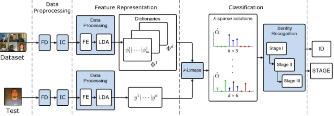
We call the proposed frameworkk-LiMapS-MFI being based on thek-LiMapS al-gorithm, and adopting both multiple Illumination Corrections (IC) and multiple Feature Extractors (FE). In the block diagram of Fig. 1 we outline it and in this section we give the insight into its first two phases.
Fig. 1. The proposed method consists of three modules.1.Data Preprocessing:based on the Face Detection (FD) and the Illumination Corrections (IC).2.Feature Representation:built on Feature Extraction (FE), projection in the LDA space, and the dictionary and test vector construction.
3.Classification:uses thek-LiMapSSR method and the multi-stage Identity Recognition module; examples of ideal sparse solutions fork= 3,6 are depicted, where the blue positions, corresponding to the right subject, are very present in the support.
2.1. Face Detection
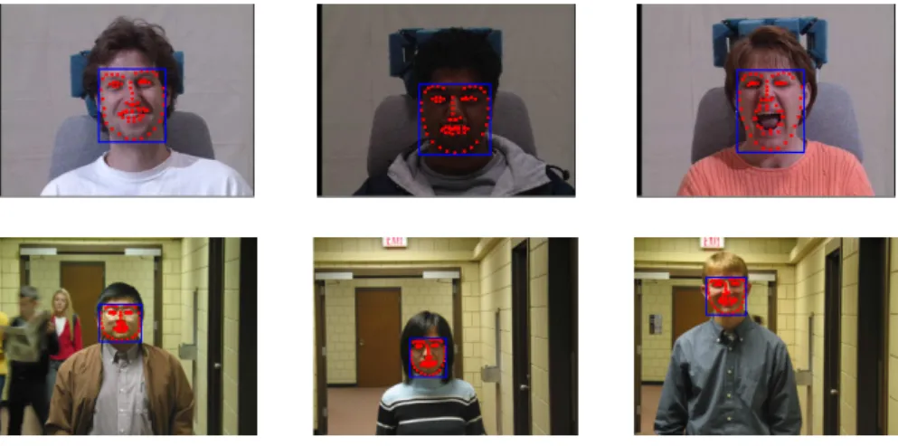
Given generic images, the very first step for an automatic FR system consists in determining in the most precise way the location and size of human faces, if any (FD in Fig.1). To this end, we apply to all the training and the test images the effective method presented in 8. Briefly, this approach, inspired by the method presented in 47, is a unified model for face detection and landmark estimation in cluttered images, with different illumination or face expressions. The approach con-sists in merging local and global information by a tree-shaped pictorial structure that characterizes and connects face landmarks. The distinctiveness of the approach presented in 8 concerns the patch characterization: while the seminal method in 47 relies on hand-crafted descriptors such as HoG responses 9, the adopted method uses a representation learnt directly from example images, that is the histograms of sparse codes (HSC) 28. This characterization allows to customize the feature de-scription, making the method particularly reliable and adaptable to the variability of face appearance (Fig. 2) contrarily to more traditional FD such as Viola-Jones 37.
For a quantitative evaluation, we measured the Root Mean Square Error (RMSE) on the landmark localization corresponding to 234 frontal images, multi
Fig. 2. Examples of FD applied to images with clutter background, affected by illumination and expression variations. First line: images of the Multi-PIE database, second line: images of the FRGC database.
expression and multi illumination, of the Multi-PIE database for which the ground truth is available. The error is normalized with respect to the face size, that is the mean of its height and width, revealing a localization error lower than the 5% of the face size on the 97% of the image set, and 100% of success accepting an error within the 10% of the face size. On all the other images referred in the experimental section (Sec. 4), we just verified that no face was missed, thus allowing the subse-quent processing. All the localized faces are automatically cropped on the bases of the found landmarks, rescaled to a size of 80×70 pixels, and passed to the next FR steps deputized to deal with possible misalignments, as it would happen in real applications.
2.2. Multi-Feature Extraction
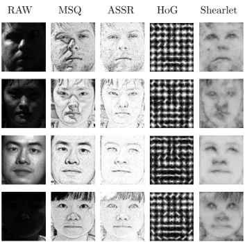
A second aspect to tackle in designing a FR system is the choice of the image rep-resentation. Many FR systems adopt one single feature, however in such a complex task it has been proven that “it is often the case that no single class of features is rich enough to capture all of the available information” 34. Here we extend this con-sideration on features to the illumination correction (IC in Fig.1) methods, being each one able to extract different discriminative information from images acquired in various illumination conditions (Fig. 3) 7. Thus,k-LiMapS-MFI takes into ac-count a pool of demonstrably effective IC methods, and feature extractors (FE in Fig.1), and combines them together obtaining a rich feature pool that makes the system more robust to a variety of possible image disruptions. Of course some of these transformations could yield misleading information, however, this is fully overcome in the classification stage, because we experimentally observed that the most informative data give rise to the strongest classifiers.
RAW MSQ ASSR HoG Shearlet
Fig. 3. Examples of IC and FE methods applied to four images of the YaleB database. Note that the MSQ adds artifacts on the first two images while enhances the last two. The two type of feature descriptions (HoG and Shearlet) are reported to highlight the different information extracted by each of them.
Formally, let IC be a set of illumination corrections and FE be a set of feature extractors, then we construct the pool F = IC×FE of combined transformations f1, ..., fd∈ F,d=|F |=|IC| · |FE|, eachfj mapping an imageIto the correspond-ing illumination-corrected feature vectorfj(I)∈Rnj.
Given the face image gallery G = {I1, . . . , Im} ⊂ RN corresponding to the subjects or classesC={1, ..., c}, after the automatic cropping and normalization, we characterize each image according to the featuresfj(I
i). To perform dimensionality reduction while preserving as much as possible the class discriminative information, we apply the LDA projectionφji =W
j
LDAfj(Ii), whereWj
LDA is the standard LDA projection matrix constructed from the combined feature vectorsfj(Ii), i= 1, ..., m. In summary, after the transformationsfj andWj
LDAeach imageIi is mapped into a (c−1)-dimensional space as shown in the diagram:
RN f j −−−−−→ Rnj W j LDA −−−−−→Rc−1 Ii 7−−−−−→fj(Ii)7−−−−−→φji
On the basis of the obtained data, we setup d distinct dictionaries, Φj ∈
R(c−1)×mby column-wise attaching the correspondingmfeature vectors, that is Φj=hφj
1| · · · |φjm
i
The multi-feature extraction process and the dictionary construction are sketched in the following pseudo-code, maintaining the variable names used in the text.
Algorithm 2.1: DictionaryConstruction(G) procedure MultiFeatureExtraction(I)
I←FaceDetection(I) I←Crop&Normalization(I) for j←1tod dofj←ApplyFeature(j, I) return (f1, . . . , fd) main for each Ii∈ G do(fi1, ..., fid)←MultiFeatureExtraction(Ii) for j←1tod do Fj←(f1j, ..., f|G|j ) WLDAj ←LinearDiscriminantAnalysis(F j) Φj←WLDAj · Fj Φ←(Φ1, . . . ,Φd)
WLDA←(WLDA1 , . . . , WLDAd )
return (Φ,WLDA)
3. Classification by sparse representation
This section is devoted to describe how the SR combined with a multi-stage classifier can effectively solve the FR problem (Classification phase in Fig. 1).
3.1. Sparse representation
Let us first introduce the general paradigm 6. Briefly, let us consider a column-vectory in the p-dimensional spaceRp representing a test sample and the matrix Φ∈ Rp×m, called dictionary, whose columns are a fixed collection of m samples, calledatoms. Let us denote thesupport of a vectorα∈Rmby supp(α) ={i:αi6= 0}. A vectorα is said to be k-sparse iff its ℓ0-norm kαk0 = |supp(α)| ≤ k. The problem of representing the sampleyby the dictionary Φ consists in solving Φα=y forα. In general, whenp≪mthe problem is underdetermined and the dictionary Φ is said to beovercomplete, so that there may exist infinitely-many solutions. In the sparse paradigm, one expects to representy with the least number of columns in Φ, and hence this leads to the central problem of noiseless sparse representation, defined as
argmin α∈Rm
This is a well-known NP-hard optimization problem 23, therefore in many ap-plication contexts it is very common to introduce the following variant, called the sparse approximation problem, where a fixed sparsity level k is guaranteed while minimizing the reconstruction errorkΦα−yk, i.e.,
argmin
α∈Rm kΦα−yk subject to kαk0≤k. (1) Within this framework, in 1 we proposed a new sparse solver, calledk-LiMapS, that adopts theℓ0-norm optimization, and is based on a suitable parametric family of Lipschitzian type mappings providing an easy and fast iterative scheme. In 2 we appliedk-LiMapSto the FR problem: projecting the raw images in the LDA space and replacing the original simplex method used in 40 with k-LiMapS, the clas-sification became much faster, and achieved higher performances than SRC. Here we extend this technique to amulti-feature andmulti-stage classification system in order to make it more accurate and enriched with the reliability degree.
Specifically, given an automatically cropped and normalized test image T ∈
RN, the corresponding dfeature vectors are computed as yj =Wj
LDAfj(T), that is projecting fj(T) through the same LDA mapping matrix defined for the jth dictionary Φj. According to the original paradigm, the problem of recognizing the identity of T among the subjects in C is recast into the problem of finding the k-sparse solutions ˆαj of thedfeature vectorsyj so that
ˆ
αj = argmin α∈Rm
kΦjα−yjk subject to kαk0≤k, j={1...d}.
This process gives rise to the pool Ak = αˆ1, . . . ,αˆd (k-sparse solutions in Fig. 1) that is further processed by the multi-stage classifier that we propose and describe in the next section.
3.2. Multi-stage classifier
Given the poolAkofdsparse solutions, the new classifier adopted in thek-LiMapS -MFI method relies on thesupports, supp(ˆαj), of all sparse solutions ˆαj, instead of using the standard residual measure as in 40 . This classification approach over-comes the weakness of Euclidean norm-based measure (at the base of the residual measure) when dealing with noisy images, improving the global recognition rates.
In this regard, the sparsity level k plays a key role since it strongly influences the discriminative power of the system. Let ¯nbe the number of samples per subject in the gallery. Experimentally we observed two scenarios. On the one hand, in case ofnon ambiguousimages, it is convenient to set a small value of sparsity, i.e.k= ¯n, producing a very efficient and precise identification. On the other hand, when even with small values ofk the support is scattered over different subjects (ambiguous
cases), larger values of k ( i.e. k = 3·¯n ) leads to a bigger chance of having a significant presence of the right subject in the selected pool.
On the basis of these considerations, we build up a cascadingmulti-stage model (Identity Recognitionin Fig. 1), where both the required sparsitykand the decision rules are progressively relaxed. This allows us to attribute a reliability degree to each estimated identity according to the stage that solved it, meaning that the earlier the identification is solved the more reliable it is. Specifically, we propose a 3-stage voting system based on the sparsity promotion worked out on the multi-feature dictionaries, where the sparsity level k is fixed, case by case, equal to a multipleq·n¯ (being, ¯nthe number of images per subject in the dictionary). STAGE I This stage aims at solving the less ambiguous cases guaranteeing both
a high reliability degree of the classifications carried out, and low compu-tational costs. To this end, we choose a small integerqIin order to require a quite high sparsity, i.e., k = qI·n¯ and we derive the k-sparse solution set Ak by applying the k-LiMapS algorithm to each dictionary Φj. Let L:{1, . . . , m} → C be the mapping from the column-indexi of Φj to the corresponding subjectL(i)∈ C, and let
VI={L(i)∈ C:i∈supp(ˆα),αˆ ∈Ak}
be the multiset of votes collected from all members of Ak. Given u dis-tinct subjectss1, . . . , su in VI ordered according to their relative frequen-cies f r(si) such that f r(s1)≥f r(s2)≥ · · · ≥f r(su), then the identity is provided by the statement
ID(T) =s1 ⇔ f r(s2)
f r(s1) < σI, (2)
where σI ∈ (0,1) is a suitable threshold (see Sec. 4.1 for the statistical analysis set up to deriveσI). If the condition is not satisfied, the decision process passes to the next stage.
STAGE II This stage aims at classifying the unsolved cases of STAGE I, even if both reliability and efficiency may deteriorate. Specifically, in this stage we compute a pool of sparse solutions denoted by A = S
k∈KAk, being K = [qIn, ..., q¯ II¯n] a set of integers equally distributed, defined on the basis of the two parametersqIandqII. Analogously to STAGE I, we collect the votes
VII={L(i)∈ C:i∈supp(ˆα),αˆ ∈ A},
and we apply the rule (2) with a weaker threshold, namelyσII∈(0,1), to determine the subject identity of the test image. If a decision is not taken here, the process goes on to the next stage.
STAGE III In this last stage we refer to the votes collected in VII and apply a further relaxed version of rule (2), setting σIII = 1, thus accepting any identitys1 as long as it has the highest relative frequencyf r(s1):
This stage leaves unclassified only the rare cases (< 0.1% of the tested images) where the previous inequality is not satisfied, implying that there is an ex aequo, that is a misclassification.
The overall method is sketched in the Algorithm 3.1, adopting when possible the same variable names used in the text.
3.3. Reliability and Consistency
Having defined a 3-stage classifier, we attribute to each stage a confidence level defining a reliability and a consistency degree with the following meaning.
Reliability: denoted byρ, is the ratio between the number of correct classifications and the number of test images classified by the stage (quality measure). Consistency: denoted by γ, is the percentage of images classified by the stage
(quantitative measure).
The reliability of any test image classification is then set equal to the reliability of the stage that produced it. This approach provides a more fine-grained decisional tool with respect to that provided by the solely total recognition rate, usually adopted.
Naturally, reliability and consistency vary according to both the properties of the referred gallery (n. of subjects, image quality, etc), and to the parameter settings
as investigated in the next section.
Algorithm 3.1: k-LiMapS-MFI(T,G, K, σI, σII)
comment:the following procedure is computed offline {Φ,WLDA} ←DictionaryConstructon(G)
comment:sparsification of the image T
(fT1, . . . , fTd)←MultiFeatureExtraction(T) forj←1tod doTLDAj ←W j LDA·f j T
comment:multi-stages classification of the image T
forj←1tod doαˆj←k-LiMapS(Φj, Tj LDA, K(1)) Ak←( ˆα1, . . . ,αˆd) VI← {L(i)∈ C:i∈supp( ˆα),αˆ∈Ak} {f r, sbj} ←SortDescent(VI) iff r(2)/f r(1)< σI then ID←First(sbj) STAGE←1 else for i←1to|K| do k←K(i) for j←1tod doαˆjk←k-LiMapS(Φj, TLDAj , k) Ak←( ˆα1k, . . . ,αˆdk) A ←S k∈KAk VII← {L(i)∈ C:i∈supp( ˆα),αˆ∈A} {f r, sbj} ←SortDescent(VII) ID←First(sbj) if f r(2)/f r(1)< σII thenSTAGE←2 elseSTAGE←3
return(ID,STAGE)
4. Experiments
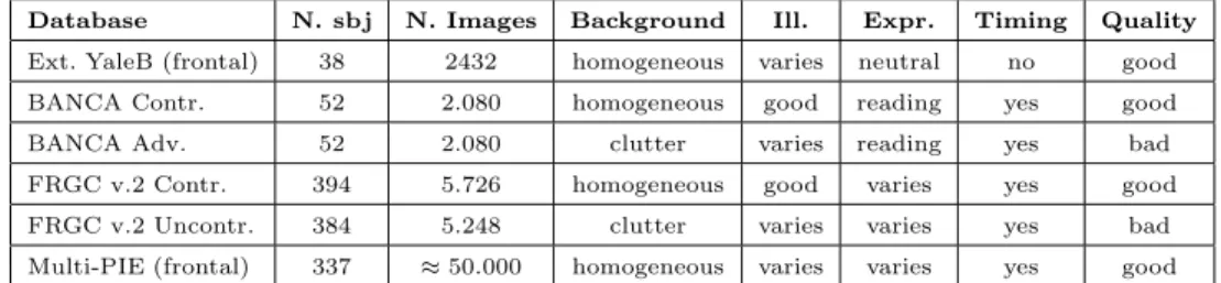
In order to test thek-LiMapS-MFI algorithm against various combinations of un-controlled conditions (e.g. different illuminations, backgrounds, expressions, and poses), we take into account several public databases: frontal faces of Extended YaleB, BANCA Controlled and Adverse, FRGC v2.0 Controlled and Uncontrolled, and frontal faces of Multi-PIE (in Table 1 we synthesize their peculiar characteris-tics).
The images are preprocessed according to Sec. 2.1, rescaled to 80x70 pixels, and transformed applying a pool of IC and FE on them. In particular we correct the illumination adopting the linear stretching, the MSQ (Multi-Scale Quotient) and
Table 1. Databases and their characteristics:N. sbj,N. Images,Background,Illumination
(varies: oriented light, over or underexposure,good: homogeneous light),Expression (neutral,
varies: neutral, smiling, screaming, or angry.reading: subjects who are reading), Timing(no: single acquisition section,yes: several sessions spanning over several months),Img Quality(good: high resolution, focused images;bad).
Database N. sbj N. Images Background Ill. Expr. Timing Quality
Ext. YaleB (frontal) 38 2432 homogeneous varies neutral no good BANCA Contr. 52 2.080 homogeneous good reading yes good BANCA Adv. 52 2.080 clutter varies reading yes bad FRGC v.2 Contr. 394 5.726 homogeneous good varies yes good FRGC v.2 Uncontr. 384 5.248 clutter varies varies yes bad Multi-PIE (frontal) 337 ≈50.000 homogeneous varies varies yes good
ASSR (Adaptive Single-Scale Retinex) techniques 38, and subsequently we extract the HoG (Histogram of Oriented Gradients) 9, Shearlet 5 and MSLBP (Multi-Scale Local Binary Pattern) features 24, resulting in nine combined-feature spaces. In Fig. 3 some examples of image preprocessing and feature extractions are shown.
We run 50 trials on every above mentioned datasets, where in each trial we ran-domly select ¯nimages per subject to form the dictionaries and split the remaining ones into validation and test sets. We emphasize that, as it could happen in real applications, no particular constraint is given for the gallery construction, where any illumination or expression are accepted.
4.1. Settings
On the basis of a tuning session, the parameters used in illumination correction and feature extraction have been set as follows. In MSQ we adopt Gaussian fil-ters with four standard deviations in the range σ ∈ (1,1.6). In ASSR the num-ber of iterative convolutions is set to 10 and the weights needed for the filter are δ = 10e−Ex,y[|∇I(x,y)|]/10 (that is based on the expected value of the image gra-dient), and h = 0.1e−10τ, with τ being the normalized average of local intensity differences. Concerning the HoG features, we refer to 15×15 patches, concatenat-ing the obtained 8-bin histograms. In MSLBP we maintain the same window and histogram sizes as in HoG, setting the circle radius equal to 1,3,5, respectively. The shearlet feature has been implemented using the Meyer-type filter, and adding together the detail coefficients, while excluding the first scale (low frequencies).
Regarding the parameters involved in the classification phase, we set them as follows.
• Aiming at testing the system in the challenging case of small sample size dictionaries, we set ¯n= 3 or ¯n= 5.
• We set qI and the values of K (defined in the previous section) directly proportional to the number of subjects c in the dictionary, so that, when
processing large dictionaries, the system has a greater chance of selecting the correct subject. This is motivated by the fact that the more populous the dictionary is, the more the support ofk-LiMapSsolution scatters over different subjects. Specifically, for all experiments we setqI=⌈c/50⌉,qII= ⌈c/10⌉obtaining aKwith values equally distributed with step qI¯n. • In order to set adequate values for the thresholds σI and σII, we refer to
the validation sets of each considered database and conduct an empirical analysis based on the ratiosf r(s2)/f r(s1) as defined in rule (2). Regarding σI, we report the average ratios in the two cases, corresponding to whether s1 is or is not the correct identity (see column group VI in Table 2). It should be noted that the correct and wrong identifications are very well separated in all the datasets, allowing us to say that σI is not a critical threshold. We hence set it to a trade-off value between Avg+Std of the correct case and Avg−Std of the wrong case, referring to the last row of Table 2, that is σI = 0.4. Once σI is fixed, we can establish which test images fall in STAGE II applying rule (2), and carry out the same analysis as the previous one, leading to the average ratios we report in Table 2, column groupVII. Notice that in this case, the averages are closer to each other, but still quite separated. According to this analysis, we setσII=Avg + Std of the correct case, capturing most of the correct classifications, that isσII= 0.8.
Table 2. Averages and standard deviations off r(s2)/f r(s1) in STAGES I and II whens1is the
correct identity and when it is not. Tests were run for all DBs with ¯n= 3, over 50 trial validation sets.
VI VII
s1correct s1wrong s1correct s1wrong
DB Avg Std Avg Std Avg Std Avg Std
Ext. YaleB (frontal) 0.10 0.15 0.70 0.24 0.68 0.16 0.79 0.15 BANCA Contr. 0.05 0.10 0.70 0.24 0.70 0.15 0.79 0.12 BANCA Adv. 0.06 0.10 0.68 0.23 0.71 0.17 0.83 0.14 FRGC Contr. 0.24 0.12 0.81 0.16 0.63 0.13 0.85 0.12 FRGC Uncontr. 0.34 0.20 0.78 0.19 0.68 0.15 0.84 0.13 Multi-PIE (frontal) 0.32 0.18 0.79 0.18 0.67 0.15 0.84 0.12 Averages 0.19 0.14 0.74 0.21 0.68 0.15 0.82 0.13 4.2. Results
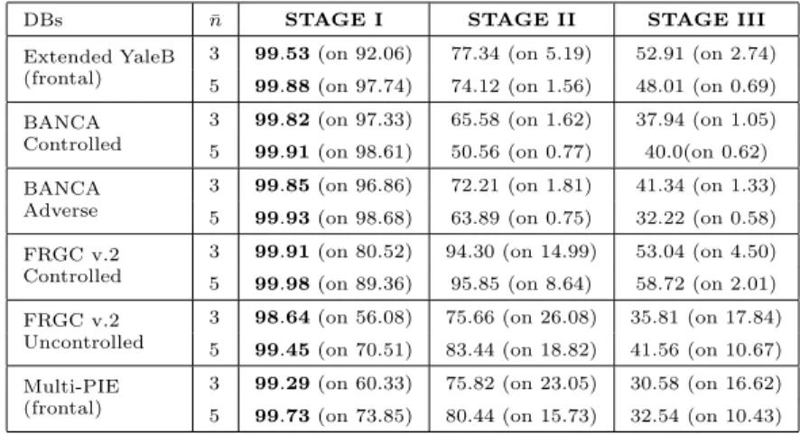
In Table 3 we report the average reliability and consistency degrees obtained run-ning thek-LiMapS-MFI over the 50 validation sets.
Table 3. For each database and for each stage we report the degrees of reliability,ρ, and consistency, γ, expressed as:ρ% (onγ%).
DBs ¯n STAGE I STAGE II STAGE III
Extended YaleB (frontal)
3 99.53(on 92.06) 77.34 (on 5.19) 52.91 (on 2.74) 5 99.88(on 97.74) 74.12 (on 1.56) 48.01 (on 0.69) BANCA
Controlled
3 99.82(on 97.33) 65.58 (on 1.62) 37.94 (on 1.05) 5 99.91(on 98.61) 50.56 (on 0.77) 40.0(on 0.62) BANCA
Adverse
3 99.85(on 96.86) 72.21 (on 1.81) 41.34 (on 1.33) 5 99.93(on 98.68) 63.89 (on 0.75) 32.22 (on 0.58) FRGC v.2
Controlled
3 99.91(on 80.52) 94.30 (on 14.99) 53.04 (on 4.50) 5 99.98(on 89.36) 95.85 (on 8.64) 58.72 (on 2.01) FRGC v.2
Uncontrolled
3 98.64(on 56.08) 75.66 (on 26.08) 35.81 (on 17.84) 5 99.45(on 70.51) 83.44 (on 18.82) 41.56 (on 10.67) Multi-PIE
(frontal)
3 99.29(on 60.33) 75.82 (on 23.05) 30.58 (on 16.62) 5 99.73(on 73.85) 80.44 (on 15.73) 32.54 (on 10.43)
certainty, and it is guaranteed for a consistent part of the test images (γ > 86% on average). STAGE II, and even more STAGE III, are invoked rarely on datasets with few subjects, while they are of great help in case of uncontrolled images, solving the most ambiguous cases. These refinements entail higher computational costs and lower reliability. In practical applications, depending on the reliability required, the end user will decide which stage to consider satisfactory, implying that images solved by the others should require further process.
Unlike the reliability which is invariably high in all datasets, consistency vari-ability is more noticeable, showing that its level in STAGE I decreases with the increase of the number of subjects in the gallery, above all in presence of uncon-trolled conditions. This happens because in these cases the point scattering in the LDA space remains too high, resulting in badly-separated clusterings, and also be-cause high dimensionality of the linear system (1) diminishes the chance of achieving high discriminative sparse solutions, as required in STAGE I.
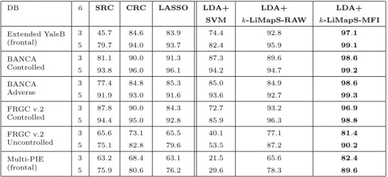
In test phase, we run the k-LiMapS-MFI on the test sets, producing the aver-agebrecognition rates reported in Table 4. For comparison in the sparse recognition domain, we report the performances obtained on the same data by well known SR methods such as SRC 40, CRC 44, and LASSO 35. In addition, we run a method using the LDA combined with SVM 19, aiming at investigating the contribute of the LDA independently from thek-LiMapSalgorithm. We also run thek-LiMapSon raw images as in 2, and report the results in Table 4, column LDA+k-LiMapS -RAW; this allows us to investigate the enhancement given by both FE, multi-IC and the support-based criterion adopted in ourk-LiMapS-MFI classifier. To set a fair comparison, we report the best performances of the competitor algorithms
b
obtained correcting the images with either the linear normalization, the MSQ, or the ASSR method. In addition, for the CRC andk-LiMapS-RAW we run several tests in order to tune, case by case, the optimal feature space dimensionality.
Table 4. Face recognition rates (%) produced on several databases, and averaging over 50 trials.
DB n¯ SRC CRC LASSO LDA+ LDA+ LDA+
SVM k-LiMapS-RAW k-LiMapS-MFI Extended YaleB (frontal) 3 45.7 84.6 83.9 74.4 92.8 97.1 5 79.7 94.0 93.7 82.4 95.9 99.1 BANCA Controlled 3 81.1 90.0 91.3 87.3 89.6 98.6 5 93.8 96.0 96.1 94.2 94.7 99.2 BANCA Adverse 3 77.4 84.8 85.3 85.0 84.9 98.6 5 91.9 93.0 91.6 93.6 92.7 99.3 FRGC v.2 Controlled 3 87.8 90.0 84.3 72.7 93.2 96.9 5 94.4 95.0 92.8 85.9 96.3 98.8 FRGC v.2 Uncontrolled 3 65.6 73.1 65.5 40.1 77.1 81.4 5 75.1 82.8 79.6 53.5 87.2 90.2 Multi-PIE (frontal) 3 63.2 68.4 63.1 21.5 65.6 82.4 5 75.9 80.6 76.2 29.6 78.3 89.6
Analyzing the results, we observe that, independently of the database, the k -LiMapS-MFI system obtains the best global performances in terms of recognition rates in all the experiments. Comparing thek-LiMapSperformances over the dif-ferent DBs, we observe that the most challenging DBs (last two in Table 4) achieve the lowest performances, and they are more influenced by the number of images per subject, yielding a significant gap between the case ¯n= 3 and ¯n= 5. This result is expected since we observed lower consistency on STAGE I as shown in Table 3.
As final note on the recognition ability, according to the experimental results reported in Table 4, we can assert that combining multi-FE and multi-IC data in LDA spaces, together with the support-based criterion is an effective strategy. Indeed, this approach leads to significant performance improvements with respect to both other standard sparse coding FR systems (SRC, CRC, and LASSO), and to other methods applied on raw data and relying on LDA projection, such as LDA + SVM, and LDA +k-LiMapSwith the residual criterion.
In regard to the computational time, we observe that it varies according to the gallery cardinality, the number of images per subject, and the stage that solves the subject identity. In particular, with regard to the average execution time of the classification phase only, STAGE I ranges from 0.002s (on the ext. YaleB database with ¯n = 3 images per subject in the dictionaries) up to 0.03s (on the FRGC v.2 Controlled database with ¯n= 5 images per subject in the dictionaries). Concerning STAGE II it requires from 2.3 (on the smallest dictionaries) up to 8.6 (on the most populous dictionaries) times the computational time of the corresponding STAGE I.
All the experiments were executed in MATLAB R2012a on an Intel Core i5 3.5GHz machine with 8GB RAM.
5. Conclusions
Despite the face recognition task has seen great breakthroughs in the last years, the problem is still open, and a big effort is yet devoted to tackle it in the most adverse conditions. In this paper we focus on two challenge conditions that hinder most of the FR systems: the small sample size problem, that is small number of images per subject in the gallery, and uncontrolled conditions, concerning simultaneously pose, lighting, expressions and image quality. Moreover, inspired by the HVS we equipped our FR system with a reliability degree, that is a measure of confidence that helps in deciding to what extent one can trust in the identification obtained by the system at hand, as humans do.
The proposed framework, namelyk-LiMapS-MFI method, is based on the well established sparse representation paradigm. It takes into account a pool of demon-strably effective illumination correction methods and feature extractors, to obtain a rich feature pool that makes the system more robust to a variety of possible image disruptions. The multi-features are then projected in the highly discriminative LDA space, where the classification phase is realized by a cascading multi-stage scheme. This approach providesi)an overall very good performance compared to other experimented methods, andii) a high reliability recognition rate for the most part of the tested images, which can be very informative in real-world applications.
Experiments conducted over different public databases show that the multi-feature representation in the LDA spaces, together with the sparse representation is an effective strategy. Indeed, in all the experiments,k-LiMapS-MFI system obtains the best global performances in terms of recognition rates with respect to both other standard sparse coding FR systems (SRC, CRC, and LASSO), and other methods relying on LDA projection, such as LDA + SVM, and LDA +k-LiMapSwith the residual criterion.
References
1. A. Adamo and G. Grossi. A fixed-point iterative schema for error minimization in k-sparse decomposition. InProc. of the IEEE Inter’l Symposium on Signal Processing and Information Technology (ISSPIT ’11), pages 167–172, 2011.
2. A. Adamo, G. Grossi, and R. Lanzarotti. Sparse representation based classification for face recognition by k-limaps algorithm. InImage and Signal Processing - 5th Int’l Conf., ICISP 2012, volume 7340 ofLecture Notes in Computer Science, pages 245– 252. Springer, 2012.
3. S. Arca, P. Campadelli, R. Lanzarotti, G. Lipori, F. Cervelli, and A. Mattei. Improving automatic face recognition with user interaction.Journal Forensic Sci, 57(3):765–771, 2012.
4. K. Ayarpadi, E. Kannan, R. R. Nair, T. Anitha, R. Srinivasan, and P. Scholar. Face Recognition under Expressions and Lighting Variations using Masking and
Synthesiz-ing.Int’l Journal of Engineering Research and Applications (IJERA), 2(1):758–763, 2012.
5. M. Borgi, D. Labate, M. E. Arbi, and C. Amar. Shearlet network-based sparse coding augmented by facial texture features for face recognition. LNCS of Proc of ICIAP Conference, 8157:611–620, 2013.
6. E. Candes, J. Romberg, and T. Tao. Stable signal recovery from incomplete and inaccurate measurements.Comm. Pure Appl. Math, 59(8):1207–1223, 2005.
7. H. Chen, P. Belhumeur, and D. Jacobs. In search of illumination invariants.Proc. Int.l Conf on Computer Vision and Pattern Recognition (CVPR), 1:254–261, 2000. 8. V. Cuculo, R. Lanzarotti, and G. Boccignone. Using sparse coding for landmark
localization in facial expressions. InProc. of Int’l Conf. EUVIP. IEEE, 2014. 9. N. Dalal and B. Triggs. Histograms of oriented gradients for human detection.Proc.
of IEEE Conference on Computer Vision and Pattern Recognition, 1:886 – 893, 2005. 10. W. Deng, J. Hu, J. Guo, W. Cai, and D. Feng. Emulating biological strategies for
uncontrolled face recognition.Pattern Recognition, 43(6):2210–2223, 2010.
11. W. Dong, L. Zhang, G. Shi, and X. Wu. Image deblurring and supper-resolution by adaptive sparse domain selection and adaptive regularization.IEEE Transactions on Image Processing, 20(7):1838 – 57, 2011.
12. S. Gao, I. Tsang, and L. Chia. Sparse representation with kernels.IEEE Transactions on Image Processing, 22(2):423–434, 2013.
13. R. Gopalan and D. Jacobs. Comparing and combining lighting insensitive approaches for face recognition. Computer Vision and Image Understanding, 114(1):135–145, 2010.
14. R. He, W. Zheng, and B. Hu. Maximum correntropy criterion for robust face recog-nition. IEEE. Trans. Pattern Analysis and Machine Intelligence, 33(8):1561–1576, 2011.
15. T. Huang, Z. Xiong, and Z. Zhang. Face recognition applications. In S. Z. Li and A. K. Jain, editors,Handbook of Face Recognition, pages 617–638. 2011.
16. C. Huo, R. Zhang, D. Yin, Q. Wu, and D. Xu. Hyperspectral data compression using sparse representation. In Hyperspectral Image and Signal Processing: Evolution in Remote Sensing (WHISPERS), 2012.
17. Z. Jiang, G. Zhang, and L. Davis. Submodular dictionary learning for sparse coding.
Proc. of IEEE Conference on Computer Vision and Pattern Recognition, pages 3418– 3425, 2012.
18. M. Ko¸c and A. Barkana. A new solution to one sample problem in face recognition using FLDA.Applied Mathematics and Computation, 217(24):10368–10376, 2011. 19. J. Li, B. Zhao, H. Zhang, and J. Jiao. Face recognition system using svm classifier
and feature extraction by pca and lda combination. InInt’l Conf. on Computational Intelligence and Software Engineering, 2009. CiSE 2009, pages 1–4. IEEE, 2009. 20. C. Lu and X. Tang. Surpassing human-level face verification performance on LFW
with gaussianface.AAAI, 2015.
21. A. Nabatchian, E. Abdel-Raheem, and M. Ahmadi. Illumination invariant feature extraction and mutual-information-based local matching for face recognition under illumination variation and occlusion.Pattern Recognition, 44(10-11):2576–2587, 2011. 22. P. Nagesh and B. Li. A compressive sensing approach for expression-invariant face recognition. Proc. Int’l Conf. on Computer Vision and Pattern Recognition, pages 1518–1525, 2009.
23. B. K. Natarajan. Sparse Approximate Solutions to Linear Systems.SIAM Journal on Computing, 24:227–234, 1995.
invariant texture classification with local binary patterns.IEEE Transactions on pat-tern recognition and Machine Intelligence, 24(7):971–987, 2002.
25. V. Patel, T. Wu, S. Biswas, P. Phillips, and R. Chellappa. Dictionary-based face recog-nition under variable lighting and pose.IEEE Transactions on information forensics and security, 7(3):954–965, 2012.
26. L. Qiao, S. Chen, and X. Tan. Sparsity preserving discriminant analysis for single training image face recognition.Pattern Recognition Letters, 31(5):422–429, 2010. 27. J. Rabia and R. Hamid. A survey of face recognition techniques.Journal of
Informa-tion Processing Systems, 5:41–68, 2009.
28. X. Ren and D. Ramanan. Histograms of sparse codes for object detection. InProc. of CVPR. IEEE, 2013.
29. W. Schwartz, H. Guo, J. Choi, and L. Davis. Face identification using large feature sets.IEEE transactions on image processing, 21(4):2245–2255, 2012.
30. Q. Shit, A. Erikssont, A. van den Hengelt, and C. Shen. Is face recognition really a compressive sensing problem?Proc. of IEEE Conference on Computer Vision and Pattern Recognition (CVPR), pages 553 – 560, 2011.
31. P. Sinha, B. Balas, Y. Ostrovsky, and R. Russell. Face recognition by humans: 20 results all computer vision researchers should know about. MIT Press Cambridge, 2005.
32. Y. Sun, D. Liang, X. Wang, and X. Tang. DeepID3: Face recognition with very deep neural networks.CoRR, abs/1502.00873, 2015.
33. Y. Taigman, M. Yang, M. Ranzato, and L. Wolf. DeepFace: Closing the gap to human-level performance in face verification. InThe IEEE Conference on Computer Vision and Pattern Recognition (CVPR), June 2014.
34. X. Tan and B. Triggs. Enhanced local texture feature sets for face recognition under difficult lighting conditions.Trans. on Image Processing, 19:1635–1650, 2010. 35. R. Tibshirani. Regression shrinkage and selection via the lasso.Journal of the Royal
Statistical Society Series B (Methodological), 58, 1996.
36. A. Tolba, A. El-Baz, and A. El-Harby. Face recognition: A literature review.Int. J. Signal Process., 2:88–103, 2006.
37. P. Viola and M. Jones. Rapid object detection using a boosted cascade of simple features. Proc. IEEE Conf. Computer Vision and Pattern Recognition, 1:511–518, 2001.
38. V. ˇStruc and N. Paveˇsi´c.Photometric normalization techniques for illumination in-variance, pages 279–300. IGI-Global, 2011.
39. A. Wagner and J. Wright. Toward a practical face recognition system: Robust align-ment and illumination by sparse representation. IEEE Trans. Pattern Analysis and Machine Intelligence, 34(2):372–386, 2012.
40. J. Wright, A. Y. Yang, A. Ganesh, S. S. Sastry, and Y. Ma. Robust face recognition via sparse representation. IEEE Trans. Pattern Analysis and Machine Intelligence, 31(2):210–27, 2008.
41. J. Xu, G. Yang, Y. Yin, H. Man, and H. He. Sparse-representation-based classification with structure-preserving dimension reduction.Cognitive Computation, 6(3):608–621, 2014.
42. Y. Xu, D. Zhang, J. Yang, and J. Yang. A two-phase test sample sparse representation method for use with face recognition.EEE Transactions on Circuits and Systems for Video Technology, 21(9):1255–1262, 2011.
43. S. Yan, H. Wang, J. Liu, X. Tang, and T. Huang. Misalignment-robust face recogni-tion.IEEE transactions on image processing, 19(4):1087–96, 2010.
representa-tion: Which helps face recognition?Proc. IEEE Int. Conf. on Computer Vision, pages 471–478, 2011.
45. S. Zhang, H. Yao, H. Zhou, X. Sun, and S. Liu. Robust visual tracking based on online learning sparse representation.Neurocomputing, 100:31 – 40, 2013.
46. W. Zhao, R. Chellappa, P. Phillips, and A. Rosenfeld. Face recognition: A literature survey.ACM, Computing Surveys, 35(4):399–458, 2003.
47. X. Zhu and D. Ramanan. Face detection, pose estimation, and landmark localization in the wild. InProc. of CVPR, pages 2879–2886. IEEE, 2012.
48. L. Zini, N. Noceti, G. Fusco, and F. Odone. Structured multi-class feature selection with an application to face recognition.Pattern Recognition Letters, 55:35–41, 2015.