Combining transductive and active learning to improve object-based classification of remote sensing images

(1)

Combining transductive and active learning to improve

object-based classification of remote sensing images

F´

abio N´

or G¨

uttler, Dino Ienco, Pascal Poncelet, Maguelonne Teisseire

To cite this version:

F´

abio N´

or G¨

uttler, Dino Ienco, Pascal Poncelet, Maguelonne Teisseire.

Combining

transductive and active learning to improve object-based classification of remote

sens-ing images.

Remote Sensing Letters, Taylor and Francis, 2016, 7 (4), pp.358-367.

<

10.1080/2150704X.2016.1142678

>

.

<

lirmm-01275515

>

HAL Id: lirmm-01275515

https://hal-lirmm.ccsd.cnrs.fr/lirmm-01275515

Submitted on 17 Feb 2016

HAL is a multi-disciplinary open access archive for the deposit and dissemination of sci-entific research documents, whether they are pub-lished or not. The documents may come from teaching and research institutions in France or abroad, or from public or private research centers.

L’archive ouverte pluridisciplinaire HAL, est destinée au dépôt et à la diffusion de documents scientifiques de niveau recherche, publiés ou non, émanant des établissements d’enseignement et de recherche fran¸cais ou étrangers, des laboratoires publics ou privés.

(2)

Combining transductive and active learning to improve

object-based classi

ﬁ

cation of remote sensing images

Fabio N. Güttler a,b_{, Dino Ienco}b_{, Pascal Poncelet}c_{and Maguelonne Teisseire}b

a_{ICube, Université de Strasbourg, Strasbourg, France;}b_{UMR TETIS, Irstea, Montpellier, France;}c_LIRMM,

Université de Montpellier, Montpellier, France

ABSTRACT

In this letter, we propose a new active transductive learning (ATL) framework for object-based classification of satellite images. The fra-mework couples graph-based label propagation with active learning (AL) to exploit positive aspects of the two learning settings. The transductive approach considers both labelled and unlabelled image objects to perform its classification as they are all available at training time while the AL strategy smartly guides the construction of the training set employed by the learner. The proposed framework was tested in the context of a land cover classification task using RapidEye optical imagery. A reference land cover map was elaborated over the whole study area in order to get reliable information about the per-formance of the ATL framework. The experimental evaluation under-lines that, with a reasonable amount of training data, our framework outperforms state of the art classification methods usually employed in thefield of remote sensing.

ARTICLE HISTORY

Received 17 July 2015 Accepted 9 January 2016

1. Introduction

Data labels are usually difficult and expensive to obtain. Standard classification techniques heavily rely on the hypothesis that a big quantity of labelled examples (training set) is available to build predictive models. Considering the remote sensing domain, in particular the object-based image classification, the label acquisition constitutes a time and effort consuming task for the expert. The collection of such labels can affect negatively the image classification task from two points of view: the quantity of labelled data commonly needed by standard inductive classifier and the way the objects to label are chosen.

Classical supervised inductive classiﬁcation approaches (i.e. Support Vector Machine (SVM), Naive Bayes (NB), Random Forest (RF), etc.) require many labelled data to train the model. Also, they assume that training and test data are not available at the same time since the model they have learnt needs to be enough general to classify new unseen examples available in a near future (Vapnik 1998). However, in the case of remote sensing image classiﬁcation, training examples are limited and all the objects (training and test) are available at the same time.

A diﬀerent classiﬁcation setting is supplied by transductive learning (Joachims 1999), which belongs to the family of the semi-supervised approaches. Transductive learning tries

CONTACTFabio N. Güttler [email protected]

REMOTE SENSING LETTERS, 2016 VOL. 7, NO. 4, 358_–367

http://dx.doi.org/10.1080/2150704X.2016.1142678

(3)

to propagate information from the labelled data to the unlabelled one leveraging the availability of training and test data at the same time. These kinds of techniques offer an effective approach to supply contextual classification of unlabelled examples by using a relatively small set of labelled examples. Many real-world applications can be modelled through a transductive setting. In particular, it has been also applied in the remote sensing domain (Sun et al.2014) where labels are difficult to obtain and the classification decisions should not be made separately from learning the current data. Differently from inductive classification, transductive learning does not produce any reusable model.

The second issue regards the way labels are collected. Objects which are usually labelled almost randomly by an expert while choosing examples guided by the needs of the classifier can drastically improve classification performance (Demir, Minello, and Bruzzone2014). This kind of technique is called active learning (AL), and it allows to involve expert interaction during the classifier construction. More in detail, the choice of the objects to label is guided by the learner needs; therefore, labels are obtained for the objects that can, potentially, improve the performance of the model. The objects are generally selected considering the classifier uncertainty over the set of possible examples to choose (Fu, Zhu, and Li2013). In remote sensing applications, this approach is getting more and more attention (Demir, Minello, and Bruzzone2014) due to the improvement it can supply in the task of image classification.

In this letter, we propose to couple transductive and AL in order to design a new active transductive learning (ATL) framework. We adapted a label propagation approach (Liu and Chang 2009) to object-based image classification and combined it with an effective AL strategy. The proposed methodology was experimented in the context of land cover object-based image classification.

2. Study area and data set description

2.1. Study area

Experiments were performed on theLower Aude Valleysite, located in the south of France. Spanning over a coastal wetland area of about 4842 ha, this site is part of the European network of protection areas called Natura 2000. Most of the site (56.3%) is composed of natural and semi-natural areas, specially salt-meadows, salt-marshes and coastal lagoons. The rest (43.7%) is mainly occupied by agricultural parcels (vineyards, cereal crops, orchards) and some small built-up areas (roads and houses).

2.2. Data set preparation

As input raster data we used a RapidEye multispectral image acquired in 24 June 2009 and available in the context of the Geoinformation for Sustainable Development (GEOSUD) project. The image was provided in level 3A, which means that radiometric, sensor and geometric corrections were performed. At this processing level, the RapidEye product has a pixel spacing of 5 m and containsﬁve spectral bands (approximate centre in nm): blue (475), green (555), red (657), red-edge (710) and near-infrared (805).

Image segmentation was performed using theﬁve spectral bands and considering only the area inside theLower Aude Valleysite. This step is of great importance as it provides a new and more meaningful representation of the image. Instead of the arbitrary pixel grid, segmenta-tion aims to create spatially coherent objects based on spectral and spatial features of adjacent pixels over the image. The segmentation was performed using the multiresolution

(4)

segmentation algorithm (MSA) available ateCognition Developer 8.8.1. MSA is a bottom-up segmentation based on a pairwise region merging technique. It uses a homogeneity criterion (combination of spectral and shape criteria) to decide whether to merge or not neighbouring pixels or objects. In our case, we set the MSA user parameters as following: scale = 100, shape = 0.2, compactness = 0.5. It generated a set of 13,292 objects with a good compromise in terms of under and over segmentation (Troya-Galvis et al.2015). For each object, we calculated the following attributes: mean value for thefive inner spectral bands and forfive additional spectral indices–normalized difference vegetation index (NDVI) (Rouse et al.1974), red edge normalized difference vegetation index (NDVIre) (Gitelson and Merzlyak1994; Kross

et al.2015), red edge normalized diﬀerence water index (NDWIre) (Klemenjak et al.2012), red

edge triangular vegetation index (RTVIcore) (Chen et al.2010) and simple ratio (SR) (Jordan

1969).

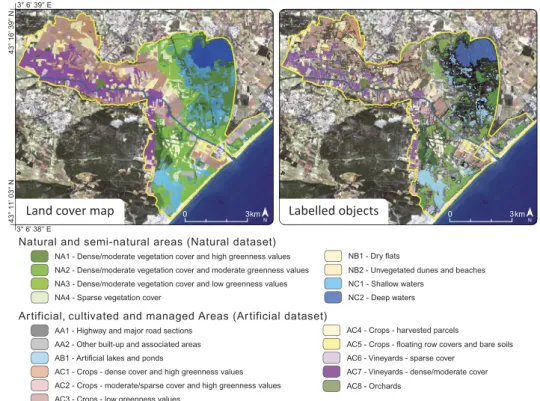
In parallel, the RapidEye image was used to create a reference map over the whole study site (seeFigure 1). This task was carried out through a manual land cover digitalization and interpretation process at the scale of 1:10,000. Field surveys and precise aerials photographs (0.5 m of spatial resolution) were employed to ensure the exactness of the land cover map. Two specific sets of land cover classes were used label the individual map units (polygons in our case). Thefirst set is specific to natural and semi-natural areas (from now called natural data set) while the second set concerns artificial, cultivated and managed areas (from now called artificial data set).

Finally, the land cover information (from the reference map) was propagated into the set of objects (from the image segmentation). Only the objects fitting completely inside the polygons of the reference map received a land cover label (see Figure 1). In total, 3357 objects were labelled for the natural data set and 3637 for the artificial data set. As the experiment reproduces a real task of land cover image classification, the number of objects

Natural and semi-natural areas(Natural dataset)

Ar tificial, cultivated and managed Areas(Ar tificialdataset)

AA1 - Highway and major road sections AA2 - Other built-up and associated areas AB1 - Artificial lakes and ponds

AC1 - Crops - dense cover and high greenness values AC2 - Crops - moderate/sparse cover and high greenness values AC3 - Crops - low greenness values

AC4 - Crops - harvested parcels

AC5 - Crops - floating row covers and bare soils AC6 - Vineyards - sparse cover

AC7 - Vineyards - dense/moderate cover AC8 - Orchards

NA1 - Dense/moderate vegetation cover and high greenness values NA2 - Dense/moderate vegetation cover and moderate greenness values NA3 - Dense/moderate vegetation cover and low greenness values NA4 - Sparse vegetation cover

NB1 - Dry flats

NB2 - Unvegetated dunes and beaches NC1 - Shallow waters

NC2 - Deep waters

0 3km 0 3km

Land cover map Labelled objects

3° 6' 39'' E

43° 16' 39'' N

3° 6' 38'' E

43° 11' 03'' N

Figure 1.Land cover reference map for the Lower Aude Valley site (left side) and the spatial

distribution of the labelled objects generated by the segmentation (right side).

360 F. N. GÜTTLER ET AL.

(5)

per class is strongly unbalanced as one can notice in the following lists (the number of objects is indicated in brackets). Natural classes: NA1(264), NA2(760), NA3(1019), NA4(161), NB1(253), NB2(155), NC1(529) and NC2(216). Artiﬁcial classes: AA1(21), AA2(418), AB1(77), AC1(439), AC2(277), AC3(658), AC4(542), AC5(209), AC6(75), AC7(900) and AC8(21).

3. Methodology

In this section, we introduce the diﬀerent components used to implement the ATL frame-work: (i) the transductive setting, (ii) the label propagation algorithm and (iii) the AL strategy.

3.1. Transductive setting

Given a set of objectsO¼f goi Ni¼1, let us denote withLthe subset of labelled objects of

O, and withUthe subset of unlabelled ones.U can have any proportion w.r.t.L, but in many real cases U is much larger than L. Every object in Lis associated to one class belonging toC¼ Cj

M

j¼1, where Mis the number of possible classes. We also denote

withYaN×Mmatrix such that the (i, j)th element of this matrix,Yij, equals 1 ifCjis the label assigned to objectoi;Yij¼0 otherwise. Without loss of generality, we can refer toL

as training data and toUas test data.

The goal of a transductive learner (TL) is to make an inference ‘from particular to particular’, i.e. given the classifications of the instances in the training setL, it aims to predict the classifications of the instances in the test set U, rather than inducing a general rule that works out for classifying new unseen instances (Vapnik 1998). Transduction is naturally related to the class of case-based learning algorithms, whose most well-known algorithm is the k-nearest neighbour (k-NN) (Joachims 2003). Differently from standard supervised setting, in the transductive setting there is no separation between model training and testing phase. The classification of new unseen example is performed at the same time the model is learnt overL.

3.2. Label propagation algorithm

In order to perform transductive learning, we adapted the approach named robust multi-class graph transduction (RMGT) proposed by Liu and Chang (2009). From the best of our knowledge, it is theﬁrst time this kind of approach is employed in a remote sensing application, in particular to perform an object-based classiﬁcation.

Essentially, RMGT implements a graph-based label propagation approach, which exploits ak-NN graph built over the entire data set to propagate the class information from the labeled to the unlabelled examples. The assumption behind this approach is that adjacent vertices are likely to have similar labels. For this reason, the label propagation procedure ensures that the classiﬁcation function varies smoothly along the edges of thek-NN graph. In the following, we describe in detail the mathematical aspects of RMGT.

Let G¼hV;E;wi be an undirected graph whose vertex set is V¼O, edge set is E¼ oi;oj joi;oj2O^sim oi;oj >0

, and edge weighting isw¼sim oi;oj

, where sim (·,·) is deﬁned as 1

1þdistð Þ; and dist(·,·) is the Euclidean distance between the feature vectors of

two objects.

Input: A collection of objectsO, with labelled objectsLand unlabelled objectsU(with

D¼L[UandL\U¼=);0

(6)

Output: A classiﬁcation overCfor the objects inU. (1) Build the similarity graphGfor the object setO.

(2) Extract thek-nearest neighbour graphGkfromG./*Section 3.2*/

(3) Build the matrixWfromGk, which represents the symmetry-favouredk-NN graph./* Section 3.2*/

(4) Compute the normalized Laplacian ofW./*Section 3.2*/ (5) Compute theRMGTsolutionF./* Equation 2 */

(6) Assign objectoi2Uto the classCjthat maximizes the class likelihood,j*= arg maxjFij.

Algorithm 1: Object-Based Transductive Classiﬁcation

Given a positive integer k, consider the k-NN graphGk¼hV;Ek;wi derived fromG

and such that E¼ di;dj

jdj 2Ni

, where Ni denotes the set of di’s k-nearest neigh-bours. A weighted sparse matrix is obtained asW¼AþAT_{, where} _A _{is the weighted}

adjacency matrix ofGkandATis the transpose ofA; the matrixWrepresents a symmetry-favoured k-NN graph (Liu and Chang2009). Moreover, letP¼IND1=2WD1=2 be the

normalized Laplacian of W, where IN is the N × N identity matrix and D = diag(W1N), where1Nis a vector of 1 s of sizeN. Without loss of generality, we can rewritePandW as subdivided into four and two submatrices, respectively:

P¼ ΔLL ΔLU ΔUL ΔUU ; Y¼ YL YU (1) whereΔLLandYLare the submatrices ofPandY, respectively, corresponding to the labelled objects. More in detail,ΔLLcontains the similarity between each pair of examples belong to

the set of labelled objects while ΔUL contains all the distances between the unlabelled

objects and the labelled one. The same analogy applies for all the other submatrices. The RMGT learning algorithmﬁnally yields a matrixF2RNM_de_ﬁ_{ned as}

F¼ Δ_UU1ΔULYLþ Δ 1 UU1j jU 1T_{j j}_UΔ_UU11j jU Nω1T_{j j}_LYLþ1Tj jUΔ 1 UUΔULYL ; (2)

whereω2RM _{is the class probability distribution that is assumed uniform.}

The learning schema used by RMGT employs spectral properties of the k-NN graph to spread the labelled information over the set of test instances. Specifically, the label propaga-tion process is modelled as a constrained convex optimizapropaga-tion problem where the labelled objects are employed to constrain and guide thefinal classification. Equation 2 represents the closed form solution of the propagation process. This equation shows how labelled (L) and unlabelled (U) examples are combined to implement the main assumption that adjacent vertices are likely to have similar labels. After the propagation step, every unlabelled objectoi is associated to a vector (i.e. theith row ofF) representing the likelihood of the objectoifor each of the classes; therefore,oiis assigned to the class that maximizes the likelihood.

Algorithm 1 sketches the main steps of the approach. Initially, the similarity matrix between all the objects is computed (Line 1). The graph-based label propagation process requires the construction of thek-NN graph (Line 2) and its symmetry-favoured transformation (Line 3). After that, the algorithm computes the normalized Laplacian of the matrix (Line 4) and the RMGT algorithm is applied on such data matrix. Line 6 describes the decision rule we adopted to perform the classiﬁcation.

(7)

3.3. Active transductive learning

AL is getting more attention in remote sensing image classification as it helps to deal with the time and effort consuming task of collecting a good quality training set to build a classification model (Demir and Bruzzone2015; Demir, Minello, and Bruzzone2014). The general AL loop (Fu, Zhu, and Li2013) involves the interaction between the classifier and the expert. Firstly a budget is defined, it represents the percentage of examples the experts is willing to label. Then the AL loop starts. At each iteration, the procedure ranks the set of unlabelled examples in order to promote in the rank the more relevant examples to label. Each example with is ranked considering its importance to the current learnt classifier. Once the rank is produced, the procedure chooses the top objects (one or more) and asks to the expert their true labels. The selected objects are added to the current training set and the classifier is updated. The AL loop stops when the budget is exhausted.

In this work, we adopted themargin-basedstrategy to score examples. This heuristic is chosen as it usually obtains better results than other uncertainty sampling methods (Fu, Zhu, and Li2013). This strategy considers the probability distribution of a classifiercon the example xover the possible set of classes C. It is prone to select instances with minimum margin between posterior probabilities of the two most likely class labels. More formally, it is defined as: marginð Þ ¼x PcðxjCfirstÞ PcðxjCsecondÞ, where given the classifierc,Pc(x|Ci) is the prob-ability of the classifiercto predict the class labelCifor the examplex,Cfirstis the most probable

class for the examplexandCsecondis the second most probable class for the classiﬁerc. Values

of margin(x) close to 0 indicate big uncertainty onxwhile values close to 1 underline reliable confidence in the prediction. In the AL step, first the unlabelled instances are ranked in ascending order w.r.t. their margin value, then the topnexamples are supplied to the expert and their true label is obtained. Wefixed the number of examples at each loop equals to 20. Considering our framework, we coupled themargin-basedheuristic with Algorithm 1. Given an object to classifyoi, we employ the likelihood vector (Fi) as posterior probability distribution to implement themargin-basedstrategy.

3.4. Experimental setting

We compared our proposal with respect to state of the art classiﬁcation approaches. As competitors we used the RF classiﬁer, the SVM and the NB approach. For SVM, we evaluated both radial basis function and polynomial kernel and, at the end, we chose polynomial kernel with exponent value equals to 8 as it supplied the best results. We coupled each of the competitors with the same AL strategy that we employed in our ATL framework (RF + AL, SVM + AL, NB + AL).

This was done in order to fairly compare our proposal with the competitors. We also investigated the benefit supplied by the AL step by comparing the performances of our ATL against the base TL. For all the competitors we used theWeka1implementation. For the RMGT a k value equals to 15 was used for building the k-NN graph. We varied the training percentage (budget) between 2% to 40% in steps of 2%. This percentage indicates the proportion of the data set that was randomly sampled to create the training set. We evaluated the classification performance using the F-measure (Gómez-Chova et al. 2011). We used F-measure instead of general accuracy due to its ability to better describe classifier perfor-mance on unbalanced data sets. We randomly initialized each classifier with an object per

(8)

class before of starting the AL process. For each pair‘classiﬁer and training percentage’we reported the average results over 30 runs.

4. Results and discussion

Classification performances over the two data sets (Natural and Artificial) of theLower Aude Valleysite are synthesized on Figure 2. As a general trend, for both data sets, we can observe that the classification performance usually improves by increasing the number of objects available in the training set.

Considering the Natural data set, we can notice that ATL outperformed all the other algorithms for any training percentage. Among the competitors, RF clearly outperformed SVM and NB. TheF-measure curves obtained for the ATL and RF approaches are similarly shaped but separated by a regular shift of almost 3 points. The NBF-measure curve has also the same general shape but the shift is around 10 points w.r.t. ATL. Conversely, the SVM curve presented a distinct shape as it becomes stable much earlier than the other approaches. With training percentages bigger than 12% only marginal improvements are obtained for SVM.

Over the artiﬁcial data set, we can observe that all the algorithms, excepted SVM, presented lower performances, for small training percentages, in comparison with the

ﬁrst data set. However, when the budget increases and reaches a reasonable percentage (equal or bigger than 20%) the general trend changes, ATL continues to improve its performance outperforming SVM. The maximum gap between ATL and SVM is around 7 points, achieved for a budget of 40%.

The two plots (b and d) ofFigure 2report the performance of our approach with and without AL. For training percentages bigger than 6% ATL clearly outperforms the base TL

0.40 0.45 0.50 0.55 0.60 0.65 0.70 0.75 0.80 0 5 10 15 20 25 30 35 40 Training Percentage (%) Artificial dataset Naive Bayes + AL Random Forest + AL Support Vector Machine + AL Active Transductive Learning

0.40 0.45 0.50 0.55 0.60 0.65 0.70 0.75 0.80 0 5 10 15 20 25 30 35 40 Training Percentage (%) Transductive Learning Active Transductive Learning 0.40 0.45 0.50 0.55 0.60 0.65 0.70 0.75 0.80 0 5 10 15 20 25 30 35 40 F -measure Training Percentage (%) Natural dataset (a) (c) (b) (d) Naive Bayes + AL Random Forest + AL Support Vector Machine + AL Active Transductive Learning

0.40 0.45 0.50 0.55 0.60 0.65 0.70 0.75 0.80 0 5 10 15 20 25 30 35 40 F -measure F -measure F -measure Training Percentage (%) Transductive Learning Active Transductive Learning

Figure 2.Classification results varying the percentage of training examples between 2% to 20% for: the Natural (left side) and the Artificial (right side) data sets. (a) All classification methods coupled with AL over the Natural data set. (b) Our framework with and without AL over the Natural data set. (c) All classification methods coupled with AL over theArtificialdata set. (d) Our framework with and without AL over theArtificialdata set.

(9)

underlining that building a training set guided by the classiﬁer needs positively inﬂuences the

final performance. Regarding smaller training percentages, we notice that the difference is very small. This fact points out that the benefit of AL only becomes evident when the training set size exceeds a minimum threshold, in our case between 6% and 8%.

In a more general evaluation, our experiments showed that the ATL framework outper-forms all the state of the art methods in both data sets. However, considering the artificial data set with training percentages smaller than 20%, the SVM + AL obtained results that differ of 2 or 3 points from the ATL. The differences in the performances can be mainly explained by the nature of the two classifiers.

For both data sets, SVM + AL quickly reaches its maximum, and then it remains stable. In thefirst iterations, the AL strategy successfully selects the optimal support vectors allowing to define the best classification hyperplane. Once those instances are included in the training set, no more examples can improve the performance as they will not modify the classification hyperplane. Instead, considering our proposal, the AL step continuously selects useful exam-ples that are employed by the transductive learner to improve the classification performance.

4.1. Per class analysis of ATL performance

In order to obtain a more accurate understanding of the ATL performances, we analysed the F-measure results per class for both data sets. This analysis is also useful to highlight some speciﬁcities of the data sets.Figure 3shows per class performance obtained using a training percentage of 20% for the natural (a) and the artiﬁcial (b) data sets.

Considering the eight classes of the natural data set, three of them presented very good performances with theF-measure values ranging from 0.80 to 0.82 (sandy areas, shallow and deep waters). Four classes (mainly related to natural vegetation areas) showed intermediate performances ranging from 0.68 and 0.76 while only one class (NA4) presented poor results with less than 0.09. This class represents areas with sparse vegetation cover and is the smallest class of this data set (161 objects). The omission errors are dramatic here as most of the NA4 objects were classified as NA3 or NB1, which corresponds to low greenness vegetation areas and dryflats, respectively. These confusions are not really surprising as the sparse vegetation cover combines small vegetation patches surrounded by bare areas. Here, we should consider the influence of over-segmented areas: instead of creating large objects including‘patches and surrounding areas’the segmentation mostly isolated such small patches into separated objects.

0.00 0.20 0.40 0.60 0.80 1.00

NA1 NA2 NA3 NA4 NB1 NB2 NC1 NC2

F

-measure

Land cover class

(a) (b) 0.00 0.20 0.40 0.60 0.80 1.00

AA1 AA2 AB1 AC1 AC2 AC3 AC4 AC5 AC6 AC7 AC8

F

-measure

Land cover class

Figure 3._F-measure values for each class obtained with the ATL framework using a training

percentage of 20%. (a) Natural data set classes. (b) Artiﬁcial data set classes.

(10)

Analysing the 11 classes of the artificial data set, we observe that two of them presented very good F-measure results (0.81 for vineyards with dense/moderate cover and 0.85 to artificial lakes and ponds). Five classes (concerning different crops and built-up areas) showed intermediate performances ranging from 0.54 to 0.68 and the four remaining classes pre-sented poor results ranging from 0.01 to 0.36. All these four classes (AC2, AC5, AC6 and AC8) are characterized by extreme omission errors. The worst of them (AC8) possesses only 21 objects and corresponds to an orchard area. Most of their objects were classified as crops

fields with vegetation (AC1 or AC3) what is somehow logical. During these periods of the year (early summer), the orchard presented a dense cover with a spectral response very near to some cereal crops. In fact, this class was created in the reference map mostly based in context andfield survey information instead of the spectral information. This is also true for the AC6 class where vineyards with sparse cover were classified sometimes as vineyards with dense cover and sometimes as harvested parcels. For the AC2 class (crops with moderate/sparse cover and high greenness values) the omission errors are clearly related to the way the reference map was constructed. Usually, each AC2 polygon in the reference map groups a set of very small and adjacent agricultural parcels separated by narrow, but very greenness, borders. However this level of generalization was not attained in the image segmentation step. Instead, it generated many small objects isolating such reduced strips of greenness vegetation from the core of the parcels. As a consequence, these objects were mainly classified as AC3 (core of the parcels) or AC1 (borders). Finally, the AC5 class, which represents cropfields with very high reflectance values (floating row covers and bare soils), was mainly classified as built-up and associated areas (AA2). This confusion is frequent in optical remote sensing as some of the materials used in civil construction can present spectral signatures close to those of bare soils andfloating row covers.

5. Conclusion

In this letter, we presented a new ATL framework that efficiently deals with object-based image classification. While standard classification techniques employ inductive learning, ATL exploits training and test sets together actively choosing new examples that can improve the final classification. The proposed approach was experimented over the Lower Aude Valley study area using a RapidEye satellite image. A reference land cover map was elaborated over the whole study area and permitted a detailed assessment of the performance of the ATL framework. The proposed approach outperformed the competitors over two data sets considering a reasonable amount of training data. As future work we would investigate more sophisticated AL techniques leveraging spatial autocorrelation. To overpass some limitations related to the generalization of the experimentalfindings we plan to extend our work over other study sites.

Note

1. http://www.cs.waikato.ac.nz/ml/weka/

Disclosure statement

No potential conﬂict of interest was reported by the authors. 366 F. N. GÜTTLER ET AL.

(11)

Funding

This work was supported by the French National Research Agency in the framework of the program‘Investissements d’Avenir’[GEOSUD project, ANR-10-EQPX-20].

ORCID

Fabio N. Güttler http://orcid.org/0000-0003-2285-4122

References

Chen, P.-F., N. Tremblay, J.-H. Wang, P. Vigneault, W.-J. Huang, and B.-G. Li.2010.“New Index for Crop Canopy Fresh Biomass Estimation.”Spectroscopy and Spectral Analysis30 (2): 512–517. Demir, B., and L. Bruzzone. 2015. “A Novel Active Learning Method in Relevance Feedback for

Content-Based Remote Sensing Image Retrieval.”IEEE Transactions on Geoscience and Remote

Sensing53 (5): 2323–2334. doi:10.1109/TGRS.2014.2358804.

Demir, B., L. Minello, and L. Bruzzone.2014.“An Eﬀective Strategy to Reduce the Labeling Cost in the Deﬁnition of Training Sets by Active Learning.”IEEE Geoscience and Remote Sensing Letters

11 (1): 79–83. doi:10.1109/LGRS.2013.2246539.

Fu, Y., X. Zhu, and B. Li.2013.“A Survey on Instance Selection for Active Learning.”Knowledge and

Information Systems35 (2): 249–283. doi:10.1007/s10115-012-0507-8.

Gitelson, A., and M. N. Merzlyak. 1994. “Spectral Reﬂectance Changes Associated with Autumn Senescence of Aesculus hippocastanum L. and Acer platanoides L. Leaves. Spectral Features and Relation to Chlorophyll Estimation.”Journal of Plant Physiology143 (3): 286–292. doi:10.1016/ S0176-1617(11)81633-0.

Gómez-Chova, L., J. Muñoz-Marí, V. Laparra, J. Malo-López, and G. Camps-Valls.2011.“A Review of Kernel Methods in Remote Sensing Data Analysis.”InOptical Remote Sensing, 171–206. Berlin: Springer. doi:10.1007/978-3-642-14212-3_10.

Joachims, T.1999.“Transductive Inference for Text Classiﬁcation using Support Vector Machines.”

InProceedings of the Sixteenth International Conference on Machine Learning (ICML-1999), Bled,

June 27–30, 200–209. Morgan Kaufmann Publishers Inc.

Joachims, T.2003.“Transductive Learning via Spectral Graph Partitioning.”InProceedings of the

Twentieth International Conference on Machine Learning (ICML-2003), Washington, DC, August

21–24, 290–297. Palo Alto, CA: AAAI Press.

Jordan, C. F. 1969. “Derivation of Leaf-Area Index from Quality of Light on the Forest Floor.”

Ecology50 (4): 663–666. doi:10.2307/1936256.

Klemenjak, S., B. Waske, S. Valero, and J. Chanussot. 2012. “Unsupervised River Detection in Rapideye Data.” In IEEE International Geoscience and Remote Sensing Symposium (IGARSS), 6860–6863. doi:10.1109/IGARSS.2012.6352587.

Kross, A., H. McNairn, D. Lapen, M. Sunohara, and C. Champagne.2015.“Assessment of Rapideye Vegetation Indices for Estimation of Leaf Area Index and Biomass in Corn and Soybean Crops.”

International Journal of Applied Earth Observation and Geoinformation34: 235–248. doi:10.1016/j.

jag.2014.08.002.

Liu, W., and S.-F. Chang.2009.“Robust Multi-Class Transductive Learning with Graphs.”InIEEE Conference

on Computer Vision and Pattern Recognition (CVPR), 381–388. doi:10.1109/CVPR.2009.5206871.

Rouse, J. W., Jr., R. H. Haas, J. A. Schell, and D. W. Deering.1974.“Monitoring Vegetation Systems in the Great Plains with ERTS.”NASA Special Publication351: 309.

Sun, Z., C. Wang, D. Li, and J. Li.2014.“Semisupervised Classiﬁcation for Hyperspectral Imagery with Transductive Multiple-Kernel Learning.”IEEE Geoscience and Remote Sensing Letters11 (11): 1991–1995. doi:10.1109/LGRS.2014.2316141.

Troya-Galvis, A., P. Gancarski, N. Passat, and L. Berti-Equille.2015.“Unsupervised Quantiﬁcation of Under- and Over-Segmentation for Object-Based Remote Sensing Image Analysis.”IEEE Journal

of Selected Topics in Applied Earth Observations and Remote Sensing 8 (5): 1936–1945.

doi:10.1109/JSTARS.2015.2424457.

Vapnik, V.1998.Statistical Learning Theory. New York: Wiley.