Advanced acceleration techniques for Nested Benders decomposition in stochastic programming

(1)

Dissertation

Advanced acceleration techniques for

Nested Benders decomposition in

Stochastic Programming

Christian Wolf, M.Sc.

Schriftliche Arbeit zur Erlangung des akademischen Grades doctor rerum politicarum (dr. rer. pol.)

im Fach Wirtschaftsinformatik eingereicht an der

Fakultät für Wirtschaftswissenschaften der Universität Paderborn

Gutachter:

1. Prof. Dr. Leena Suhl 2. Prof. Dr. Csaba I. Fábián

(2)

(3)

Acknowledgements

This thesis is the result of working for nearly four years at the Decision Support & Opera-tions Research (DS&OR) Lab at the University of Paderborn. I would like to thank those people whose support helped me in writing my dissertation.

First of all, I thank my supervisor Leena Suhl for giving me the possibility to pursue a thesis by offering me a job at her research group in the first place. Her support and guidance over the years helped me tremendously in finishing the dissertation. I also thank Achim Koberstein for introducing me to the field of Operations Research through the lecture “Operations Research A” and the opportunity to do research as a student in the field of stochastic programming. It is due to his insistence that I decided to write my computer science master’s thesis at the DS&OR Lab. I am very grateful to have Csaba Fábián as my second advisor. He not only gave valuable advice but also pointed me towards the on-demand accuracy concept. Collaborating with him has been both straightforward and effective.

My present and past colleagues at the DS&OR Lab deserve a deep thank you for the enjoyable time I had at the research group in the last years. Discussions on scientific topics were as insightful as our non-work related discussions were humorous. I would like to thank Corinna Hallmann, Stefan Kramkowski, Daniel Rudolph, and Franz Wesselmann for their time and patience in discussing implementation details and other problems that have appeared out of nowhere during the implementation of solver software. I thank my office colleague Boris Amberg for funny and interesting conversations across two monitors and for leaving the office to me until lunch.

Last but not least, I thank my family and friends, especially my parents, who believed in me and supported me. Special thanks go to my wife Pia. Finishing the thesis without her would have been much more difficult.

Paderborn, October 2013 Christian Wolf

(4)

(5)

5.2. Sequencing Protocols . . . 49 5.3. Parallelization . . . 54 5.4. Advanced Start . . . 58 5.5. Stage Aggregation . . . 58 6. Modeling Languages 61 6.1. Theoretical Concepts . . . 61 6.2. Practical Examples . . . 63 7. Required Work 67 7.1. Solver Development . . . 67 7.2. Modeling Languages . . . 68

III. Advanced Techniques and Computational Results 71 8. Accelerating the Nested Benders Decomposition 73 8.1. Cut Consolidation . . . 73 8.2. Dynamic Sequencing . . . 76 8.3. Parallelization . . . 77 8.4. Aggregation . . . 79 8.5. On-Demand Accuracy . . . 80 8.6. Level decomposition . . . 83

8.7. Extending techniques to the multi-stage case . . . 86

9. A Modeling Environment for Stochastic Programs 91 10. Computational Results 97 10.1. Test Instances . . . 97 10.2. Evaluation Techniques . . . 98 10.3. Implementation Aspects . . . 100 10.3.1. Implementation . . . 100 10.3.2. Solving a subproblem . . . 101 10.3.3. Warm Start . . . 102 10.3.4. Tolerances . . . 102 10.4. Computing environment . . . 102

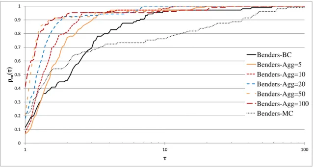
10.5. Evaluation of Two-Stage Acceleration Techniques . . . 103

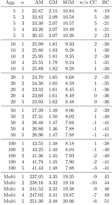
10.5.1. Cut Aggregation . . . 103

10.5.2. Cut consolidation . . . 105

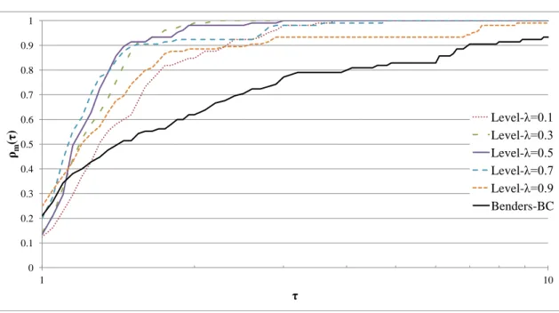
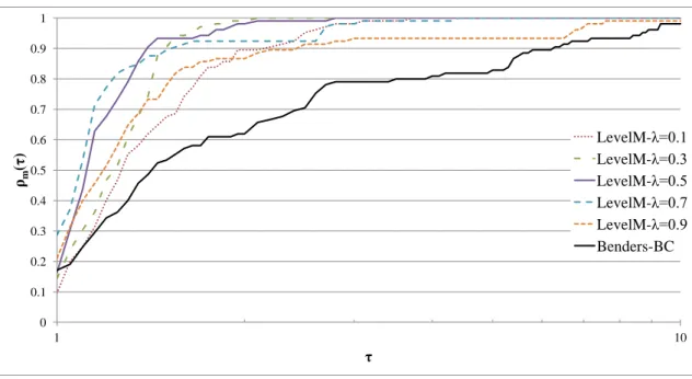
10.5.3. Level decomposition . . . 106

10.5.4. On-demand accuracy . . . 119

10.5.5. Advanced start solution . . . 132

10.6. Effect of Parallelization . . . 133

10.7. Evaluation of Multi-Stage Acceleration Techniques . . . 136

10.7.1. Sequencing protocols . . . 136

10.8. SAA and Parallel Benders . . . 140

(7)

Contents

10.9. Conclusion . . . 140

11. Summary and Conclusion 145

Bibliography 147 A. Test problems 161 B. Test Results 171 List of Figures 183 List of Tables 185 List of Algorithms 187 vii

(8)

(9)

1

1. Introduction

“Our new Constitution is now established, and has an appearance that promises permanency; but in this world nothing can be said to be certain, except death and taxes.”

— Benjamin Franklin,Letter to Jean-Baptiste Leroy

Real-world optimization problems are often modeled with traditional mathematical pro-gramming techniques. The implicit assumption, when using these tools, is that the un-derlying real-world problem is deterministic. Many real-world problems usually include uncertainty, such as uncertainty about future events, lack of reliable data, etc. The model could therefore be subject to uncertainty in its parameters or in itself, because the model is an approximation of the real-world problem and thus the optimal solution of the model may not be the optimal solution of the modeled problem.

Attempts to investigate the effects of uncertainty with traditional methods like sensitivity analysis of optimal solutions or scenario analysis, e.g., solving a deterministic model with different parameters, do not suffice to take the effect of uncertainty into account (e.g., (Wallace, 2000) and (King & Wallace, 2012, p. 2ff)). Thus to determine if uncertainty is of importance for a particular model, it has to be checked by incorporating uncertainty into the optimization problem.

Stochastic programming is a mathematical programming field that provides techniques to handle optimization under uncertainty. It is due to the early work of Dantzig (1955), Beale (1955) and Charnes & Cooper (1959). A common concept is that a decision has to be made here and now, and the uncertain future will reveal itself after that. A recourse decision can then be taken to react upon the new information.

The key questions are (King & Wallace, 2012, p. 1) • What are the important uncertainties?

• How can we handle them?

• Can we deliver valuable solutions and insights?

It is one of the main difficulties for many practical problems to deliver a solution at all, because incorporating uncertainty makes a model usually larger and harder to solve. The usage of specialized solution techniques, e.g., Benders decomposition, Progressive Hedging, Stochastic decomposition, Sample Average Approximation, etc., make practical decision problems tractable. The resulting solutions can then be examined for valuable insights. The theoretical development and practical implementation of solution techniques is therefore important to get people to use stochastic programming in the first place and thus improve their decision making capabilities. In addition, modeling tools that aid operation research

(10)

practitioners in modeling and analyzing stochastic programs are necessary to make the transition from modeling linear programs to stochastic programs possible.

The importance and widespread applicability of stochastic programming is demonstrated by its variety of application areas, including electricity, finance, supply-chain, production, telecommunications and others (see the collection edited by Wallace & Ziemba (2005)). Two recent examples demonstrate that the usage of stochastic programming leads to better decisions.

A strategic gas portfolio planning problem (Koberstein et al., 2011) determines the parameters of baseload and open contracts for gas delivery for the next gas year, where recourse actions are necessary to cover the demand during a year by using storages, open contracts and the spot market. The uncertainty of the problem is the demand, which correlates with the weather conditions. As gas is widely used for heating, colder winters generate more demand than warmer winters. Incorporating this uncertainty into the model results in an expected advantage of 5.9 million euro of the stochastic solution compared with the solution from the deterministic model. The expected solution value of the stochastic program is 182.2 million euro.

A company that owns wind power plants and hydro power plants has to schedule the plants operationally. The goal is to optimize the profit of the company, while satisfying customer demand (Vespucci et al., 2012). Excess energy generated from wind power plants can be used to pump water into higher reservoirs that can later be used by the hydro power plants. The wind depends on uncertain weather conditions and thus the power generated from wind power plants is subject to uncertainty. Vespucci et al. (2012) analyze a stochastic programming model that takes weather forecast uncertainty into account and contrast this with a deterministic model where the forecast is taken at face value. The stochastic programming model results in significant savings compared to the deterministic model.

Implementing these and other problems is easier with algebraic modeling languages that are capable of modeling stochastic programs directly. Using specialized solution methods directly after specifying the model results in either computing time savings or opens up the possibility to solve the resulting problems in the first place. Supporting and easing this process is the topic of this thesis.

The thesis is structured in three parts. The first part deals with the fundamentals. It gives an understanding of stochastic programming in Chapter 2, along with mathematical properties of these problems from which solution methods can be derived. We introduce different basic solution methods for stochastic programs with recourse in Chapter 3. In particular, we introduce the deterministic equivalent, Benders decomposition, Lagrangean relaxation, and approximative solution methods.

The second part of the thesis reviews the current state-of-the-art with respect to Ben-ders decomposition and modeling languages for stochastic programs. Chapter 4 details acceleration techniques for Benders decomposition, in particular for two-stage problems. Acceleration techniques for multi-stage problems, where Benders decomposition is applied in a nested fashion, are described in Chapter 5. An overview about challenges and devel-opments in the area of algebraic modeling languages for stochastic programs is given in Chapter 6. Given the state-of-the-art, we derive the goals of our research in Chapter 7.

(11)

3

Part III describes advanced acceleration techniques for the nested Benders decomposition algorithm and gives computational results to evaluate their effectiveness. Techniques like cut consolidation, dynamic sequencing, parallelization, different level decomposition projection problems, and on-demand accuracy are detailed in Chapter 8. Our extension of the algebraic modeling language FlopC++ to stochastic programs is described in Chapter 9. Chapter 10 contains a description of the algorithm implementation and gives extensive evaluations of the developed and implemented acceleration techniques. We conclude the contributions of this thesis in Chapter 11 and give directions for future research.

(12)

(13)

5

Part I.

(14)

(15)

7

2. Stochastic Programming Preliminaries

Stochastic programs and the needed preliminaries are introduced in this chapter. We start with mathematical programs, in particular linear and mixed-integer programs in Section 2.1. We then give some basic results in polyhedral theory that are necessary for the explanation of Benders decomposition. After that we introduce stochastic programming in Section 2.2, together with basic probability theory. Introductory texts especially for linear programming are, among others, (Vanderbei, 1997; Chvátal, 1983; Nering & Tucker, 1993). A more theoretically oriented textbook is written by Schrijver (1998). A detailed introduction to the implementation of the simplex algorithm, the main solution algorithm of linear programs used in Benders decomposition, can be found in (Maros, 2003).

2.1. Mathematical Programs

A mathematical program is an optimization problem of the following form, min f(x)

g(x)≥0 x∈ X,

where0(written in boldfont) denotes a column vector of zeroes with appropriate dimension. The functionf maps fromRn_to_R_and_g_{maps from}_Rn _to_Rm_{. The set}_{X ⊆ R}n_together with the constraintg(x)≥0defines the feasibility setFof the mathematical program. The function f is the objective function of the mathematical program. We assume throughout this thesis that the default optimization direction is minimization if not stated otherwise.

A pointx∈ Rn_{is called a solution. A solution}_x _{is feasible if}_x_{∈ X} _{and the constraints}

g(x)≥0hold, i.e.,x∈ F. Otherwise the solution is called infeasible. A solutionx∗∈ F is optimal iff(x∗)≤f(x),∀x∈ F. Note that an optimal solution does not have to be unique. A mathematical program is infeasible if the feasibility set F is empty. A mathematical program is unbounded if for every number M ∈ R there is a solution x ∈ F, such that

f(x)< M.

Mathematical programming problems are classified according to properties of the func-tions f and g and the set X. Two important categories are linear programming and mixed-integer linear programming. A linear program (LP) is a mathematical program with linear functions f and g, where X is continuous. A mixed-integer program (MIP) is a mathematical program with linear functions f and g, where X is partly continuous and partly discrete. A pure integer program (IP) is a mathematical program with linear functions f and g, whereX is discrete. A convex non-linear program has non-linear func-tions f andg, where X is convex. Quadratic programs (QPs) are an example for convex non-linear programs with a quadratic objective function f, but linear function g, where

(16)

X is continuous. The hardness of the problems differs depending on the functions and X. LP problems are in P, together with QP problems that have a positive semidefinite quadratic coefficient matrix in the objective function. General IP, MIP and QP problems areN P−hard.

We write the linear programP1 in the following matrix notation standard form min cTx

(P1) s.t. Ax≥b x≥0,

(2.1)

with right hand side vector b∈ Rm_{, objective function coefficients vector}_c_{∈ R}n_{, decision} variables vectorx∈ Rn_{and the constraint matrix}_A_{∈ R}m×n_{. To alleviate notation, in the} remainder of this thesis we will not specify which vectors we transpose, but we assume that the vectors have appropriate dimensions and are used in the transposed form if necessary. It helps in keeping the presentation clear, but concise.

A LP can also be written in the summation notation given by equation (2.2), where every decision variablexi, i= 1, . . . , nis stated explicitly.

min n X i=1 cixi s.t. n X i=1 aijxi≥bj j = 1, . . . , m xi≥0 i= 1, . . . , n. (2.2)

The matrix entry aij is the coefficient of the constraint matrix A in columniand row j. As both of the forms (2.1) and (2.2) are equivalent and differ only in notation, we use the form which is best suited to explain different concepts later in this thesis.

A more general, but equivalent form of LP (2.2) is formulation (2.3)

min n X i=1 cixi s.t. n X i=1 aijxi+xn+j =bj j = 1, . . . , m li≤xi≤ui i= 1, . . . , n+m. (2.3)

In formulation (2.3) every decision variable has a lower boundli and an upper boundui. The variablesxn+j, j= 1, . . . , m are called slack variables, because they take up the slack between Pn

i=1aijxi andbj, as we have only equalities as constraints. The three different constraint types ≥,≤ and = are modeled via the bounds on the slack variables. When the slack variable xn+j has the bounds lj = 0 and uj = ∞, it is a ≥ constraint. With the bounds lj = −∞ and uj = 0 it is a ≤ constraint. An equality is achieved with the boundslj = 0 anduj = 0, i.e., the slack variable is fixed to zero. The coefficient matrix A is necessarily of full rank, due to the slack variables. It is possible to create an equivalent LP in standard form with additional variables and/or constraints (Chvátal, 1983).

(17)

2.1. Mathematical Programs 9

An important concept that can be applied to linear programs is duality theory. Every linear program has a corresponding dual linear program; both together form a primal/dual pair. The original LP is also called the primal problem. The dual LP of the dual problem to a primal problem is again the primal problem. The dual LP D1 of the primal LP P1 (2.1) is

max by

(D1) s.t. ATy≤c y≥0.

(2.4)

A dual problem can be used to give a lower bound to the primal problem as well as the primal problem can be used to give an upper bound to the dual problem (Vanderbei, 1997, p. 51ff). We note that every feasible solution for a primal LP is at the same time an upper bound for this problem.

The following basic, but important, theorems and their proofs can be found in every LP textbook, e.g. (Vanderbei, 1997, p. 53-64). The Weak Duality Theorem (2.1) states that every feasible solution for the dual is a lower bound for the primal problem.

Theorem 2.1. Let x be a feasible solution for a primal LP P1 and y be a feasible solution for the corresponding dual LP D1. Then it holds that cTx≥by.

The Strong Duality Theorem 2.2 states that if a primal problem has an optimal solution, the corresponding dual problem also has an optimal solution, such that the objective values coincide.

Theorem 2.2. Let x∗ be an optimal solution for a primal LP P1. Then the corresponding dual LP D1 has an optimal solution y∗ such thatcTx∗=bTy∗.

Together with the Complementary Slackness Theorem (2.3), it is possible to construct these solutions from one another (Vanderbei, 1997, p. 63f).

Theorem 2.3. Let (x1, . . . , xn) be a primal feasible solution for a primal LP P. Let (y1, . . . , ym) be a dual feasible solution for the corresponding dual LP D. Let (w1, . . . , wm)

denote the primal slack variables and (z1, . . . , zn) the dual slack variables. Then x and y

are optimal for their respective problem if and only if

xizi = 0, i= 1, . . . , n

yjwj = 0, j= 1, . . . , m.

Every LP in standard form (2.1) has an associated polyhedron P := {x∈ Rn _|_Ax_≥

b, x≥0}. For the following definitions and theorems the constraint matrix is assumed to be of full rank and P 6=∅ (see (Nemhauser & Wolsey, 1999, p. 92-98) for the definitions and proofs of the theorems, (Schrijver, 1998, p. 85-107) is an alternative source). The feasible region F of an LP can be described by a finite number of extreme points and extreme rays that we define next.

Definition 2.4. A pointx∈P is called an extreme point ofP, if there do not exist points

x1, x2 ∈P, x1 6=x2, such thatx=λx1+ (1−λ)x2,0< λ <1.

(18)

r2 r1 p1 p2 p3 x1 x2 −c α

Figure 2.1.A polyhedron with extreme points and extreme rays.

Definition 2.6. A ray r∈P is an extreme ray if there do not exists raysr1, r2∈P0, r1 6=

λr2 for anyλ >0, such thatr =µr1+ (1−µ)r2,0< µ <1.

A polyhedron with extreme pointsp1, p2 and p3 and extreme rays r1 andr2 is shown in

Figure 2.1. The optimization problem associated with the polyhedron is a minimization problem, thus the objective function vector is followed in its opposed direction, namely −c. The optimization direction is depicted in Figure 2.1 by the vector −c. The angle α

betweenr1 and−cis acute, therefore−c·r1 is greater than zero andc·r1 is less than zero,

due to the equation cos(α) = _|_aa_|·|·b_b_|, with a, b∈ Rn_{\ {0}} _and_α _{being the angle between} them.

Theorem (2.7) (Nemhauser & Wolsey, 1999, p. 95), which we will use in the explanation of Benders decomposition, states that an unbounded maximization problem has an extreme ray that makes an acute angle with the objective function vector.

Theorem 2.7. If max{cx | x∈P} is unbounded P has an extreme ray r∗ withcr∗ >0.

The decomposition theorem for polyhedra (also called Minkowski-Weyl’s theorem) states that polyhedra can be represented by convex combinations of their extreme points and extreme rays (Nemhauser & Wolsey, 1999, p.96).

Theorem 2.8 (Decomposition theorem for polyhedra). The polyhedron P can be repre-sented as P =    x∈ Rn |x=X i∈I λixi+ X j∈J µjrj with X i∈I λi = 1 , λi ≥0∀i∈I, µj ≥0∀j∈J}. (2.5)

where {xi}i∈I is the set of extreme points and {rj}j∈J is the set of extreme rays of P. The Decomposition Theorem will be used in the explanation of Benders decomposition method together with the fact that every full-dimensional polyhedron has a finite number of extreme points and extreme rays.

The Minkowski-Weyl decomposition theorem can also be stated for general polyhedra, i.e.,P ={Ax≤b}andrank(A)≤n, but for that we need some more definitions (Schrijver, 1998, p. 87f).

(19)

2.1. Mathematical Programs 11

Definition 2.9. A nonempty set of points C in Euclidean space is called a cone ifλx+µy∈

C,∀x, y∈C andλ, µ≥0.

Definition 2.10. A cone C is polyhedral, if C={x | Ax≤0}.

The cone generated by the vectorsx1, . . . , xm∈ Rn is the set

cone{x1, . . . , xm}:={λ1x1+. . .+λmxm, λ1, . . . , λm ≥0}, (2.6) and is called finitely generated (Schrijver, 1998, p. 87).

Theorem 2.11 (Farkas-Minkowski-Weyl theorem). A convex cone is polyhedral if and only if it is finitely generated.

If the polyhedron has at least one extreme point, it is called pointed. A polyhedron is bounded if and only if the characteristic cone has dimension zero, i.e., char.cone ={0} (Schrijver, 1998, p. 100f). The characteristic cone is defined aschar.cone(P) ={r|Ar≤0}.

Definition 2.12. F is a face ofP if and only if there is a vectorc for whichF is the set of vectors attaining min{cx|x∈P}, provided that this minimum is finite

Finally, the Minkowski-Weyl decomposition theorem for general polyhedra is stated as follows (Schrijver, 1998, p. 88)

Theorem 2.13 (Decomposition theorem for general polyhedra). A set P of vectors in Euclidean space is a polyhedron if and only ifP =Q+C for some polytope Q and some polyhedral cone C.

In particular, the polyhedral cone C in Theorem (2.13) is the characteristic cone

char.cone(P) = {r|Ar ≤ 0} (Schrijver, 1998, p. 100). Regarding the polytope Q, it can be described with the help of the minimal faces of P, as follows.

LetF1, . . . , Frbe the minimal faces of the polyhedronP, and choose an elementxi from

Fi, fori= 1, . . . , r. Then (Schrijver, 1998, p. 106)

P =conv.hull{x1, . . . , xr}+char.cone(P). (2.7) Thus the polyhedron P can be described by a finite set of vectors {x1, . . . , xr} and its characteristic cone, which is also finitely generated.

The simplex method The well-known simplex algorithm invented by Dantzig in 1947 is one of the main solution techniques for linear programming problems. The simplex algorithm can work on the primal problem as the primal simplex or the dual problem as the dual simplex. The simplex method is an iterative method that improves a starting solution until it reaches optimality or finds that the problem is unbounded. If no starting solution can be found, the problem is infeasible. A detailed introduction to the simplex method can be found in several textbooks, e.g., (Schrijver, 1998; Vanderbei, 1997; Chvátal, 1983; Maros, 2003). Another successful approach to solve LPs is the use of interior-point methods (see the textbooks (Ye, 1997),(Vanderbei, 1997),(Schrijver, 1998), among others).

(20)

2.2. Stochastic Programs

Mathematical programs that contain uncertainties can be modeled with the use of stochastic programming techniques. Several textbooks give a good introduction into stochastic programming, both theoretical and practical (Birge & Louveaux, 2011; Kall & Wallace, 1994; Ruszczyński & Shapiro, 2003; Kall & Mayer, 2010; Shapiro et al., 2009). An overview about the application of stochastic programming is given in the volume edited by Wallace & Ziemba (2005). A book about modeling stochastic programs was recently published (King & Wallace, 2012).

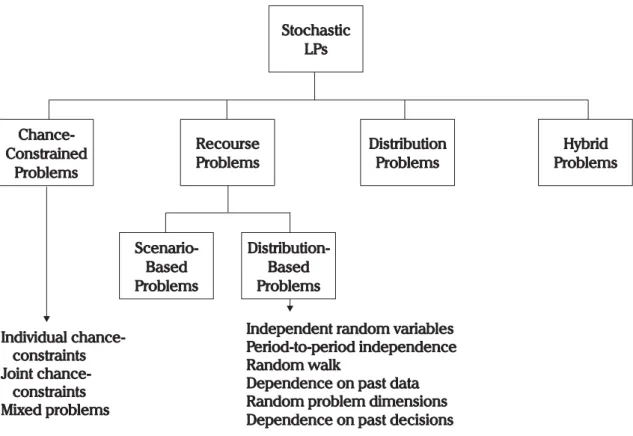
In this thesis we restrict ourselves to recourse problems whereas stochastic programming in general also handles problems with chance-constraints as well as distribution problems and combinations of these. A survey by Gassmann (2007) shows that the majority of stochastic problems are recourse problems. We present the taxonomy given by Gassmann & Ireland (1996) in Figure 2.2.

Figure 2.2.A taxonomy of stochastic LPs (Figure 3 in (Gassmann & Ireland, 1996)) A recourse problem is divided in several stages, where every stage except the first marks the realization of some uncertain parameters, but where the decision maker knows the distribution of the uncertain parameters. The first-stage marks decisions that have to be taken before any parameters become known to the decision maker. At the beginning of the second stage, some uncertain parameters are revealed and the decision maker is faced with this outcome and his former first-stage decision. The decision maker reacts with a second-stage or recourse decision to the revealed outcome. If the problem is a multi-stage

(21)

2.2. Stochastic Programs 13

problem, this process is repeated until the last stage. The goal of the decision maker is to minimize the objective function value of the first-stage decision and the expected value of the objective function value of the second-stage decision. We stress that the decision maker has knowledge about the distribution of the uncertain parameters but does not know the concrete realization when he has to make his decision. We assume that the distribution of the uncertain parameters is independent of the decisions we take.

In Section 2.2.1 we describe the necessary preliminaries of probability theory to un-derstand the two-stage stochastic problems explained in Section 2.2.2 and multi-stage stochastic problems described in Section 2.2.3. We end this section with basic properties of stochastic problems in Section 2.2.4.

2.2.1. Basic Probability Theory

Stochastic programs deal with uncertainty. Probability theory is an area of mathematics that formalizes uncertainty. As stochastic programming uses concepts defined in probability theory, we shortly describe the necessary ones. For a further introduction into probability theory the reader is referred to the literature (Bauer, 1991; Ross, 2004).

To formalize uncertainty, we use the mathematical concept of a probability space, which is a triplet (Ω,A, P) (Birge & Louveaux, 2011, p. 56). Ω is the set of all possible outcomes

ω of some random experiments, Ais the set of all events over Ω andP is the associated set of probabilities. The probability of an event P(A), A∈ Ais always between zero and one. It holds that 0 ≤ P(A) ≤1, P(∅) = 0 and P(Ω) = 1. The set of all events A is a

σ-algebra.

The mathematical conceptfiltrationdefined on a measurable space (Ω,A) is an increasing familyA_t⊆ A, t≥0 of sub-σ-algebras ofA, i.e.,A_t⊂ A_t₊₁ (Revuz & Yor, 2004). Defined in this way, A_t is the collection of events that can occur before or at staget.

The functionX : Ω→ Ris called a random variable if {ω |X(ω)≤r} ∈ A, ∀r ∈ R.

The cumulative distribution functionF(x) is defined as

F(x) =P{X≤x}, ∀x∈ R.

The probability mass function p(x) is used to describe the probability of X taking the value x, so p(x) = P{X = x}. A random variable X is discrete if it can only take a countable number of values. A random variable X is continuous if it can take an uncountable number of values. We say that a random variableX is distributed according to a random distribution, specified by F(x). Examples for random distributions are the Binomial distribution, Poisson distribution, Exponential distribution, Normal distribution, etc.

The expectation of a random variable X is denoted as E[X]. For a discrete random variable it can be written asE[X] =P

ω∈ΩωP{X=ω}. For a continuous random variable,

it is defined as the integralE[X] =R∞

−∞xf(x)dx, withf(·) = dxdF(x) being the probability density function (Ross, 2004).

(22)

2.2.2. Two-Stage Stochastic Programs

The general two-stage stochastic program with recourse minimizes the cost of the first-stage decision and the expected cost of the second-stage decision. It is stated as follows

z= min cx+Eξ[minq(ω)y(ω)] (2.8)

s.t. Ax=b (2.9)

T(ω)x+W(ω)y(ω) =h(ω) (2.10)

x, y(ω)≥0 (2.11)

The first-stage objective function coefficients c∈ Rn1_{, constraint matrix} _A_{∈ R}m1×n1 _and

right hand sideb∈ Rm1 _{are deterministic and not subject to uncertainty. Every different}

outcomeω∈Ω is called a scenario or realization. For any scenario ω some values in the technology matrix T ∈ Rm2×n1_{, the recourse matrix} _W _{∈ R}m2×n2_{, the right hand side} h∈ Rm2 _{or the objective function} _q_{∈ R}n2 _{may change. We can see every component of} T(ω), W(ω), h(ω), q(ω) as random variables that are influenced by the scenarioω. We can write ξ(ω) as a set of random vectors

ξ(ω) = (T1(ω), . . . , Tn1(ω), W1(ω), . . . , Wn2(ω), h(ω), q(ω)),

where Ai denotes the i−th column of matrixA. The constraints (2.10) and (2.11) hold almost surely with respect to the scenario probabilities, i.e., for allω with a probability greater than zero. It is possible to extend this formulation, e.g., by introducing integer requirements on the first- and/or second-stage. This can be done by replacing the non-negativity constraint (2.11) with the general formx∈X, y(ω)∈Y withX=Zn1

+ , Y =Z+n2.

Once we chose a realizationωand a first-stage solutionx, we know the second-stage data via ξ(ω). Then, the second-stage variables or recourse variables y(ω) have to be chosen, according to objective function and constraints. The name recourse variables derives from the observation that they(ω) variables react to the chosen first-stage variablesx and the scenario dependent second-stage dataT(ω), W(ω), h(ω) and q(ω). It is usually the case that most parts ofT, W, hand q are deterministic or scenario independent and only some data is scenario dependent.

A reformulation of problem (2.8) is the deterministic equivalent model (DEM)

z= min cx+Q(x) s.t. Ax=b

x≥0,

(2.12)

with expected second stage value function Q(x) =Eξ[Q(x, ω)] andQ(x, ω)

Q(x, ω) = min q(ω)y(ω)

s.t. T(ω)x+W(ω)y(ω) =h(ω)

y(ω)≥0.

(2.13)

As long as the random variables are discrete and finite, it is possible to formulate the two-stage stochastic problem with recourse (2.8) as the DEM, because the expected second

(23)

stage value function can be replaced by a summation, as further described in section 3.2. The second stage value function Q(x, ω) is also called recourse function andQ(x) is consequently called expected recourse function. The recourse function is defined to be−∞ if the problem (2.13) is unbounded, and ∞ if it is infeasible, as usual. For the expected recourse function, we adhere to the convention that ∞+ (−∞) =∞. In words it means that if any subproblem is infeasible, the expected recourse function takes the value ∞. This can be interpreted as a conservative approach by regarding the “bad” outcomes, i.e.,

Q(x, ω) =∞ that result from choosingx as more important (Walkup & Wets, 1967) than the “good” outcomes, i.e.,Q(x, ω) =−∞.

For the rest of this thesis we assume that we have discrete and finite random variables, as otherwise the solution methods for which we propose enhancements can not work, as multi-dimensional integration would be required. We emphasize that problems with continuous or discrete random variables can be approximated by problems with discrete and finite random variables and thus be solved approximately with approximation methods described in this thesis in Section 3.5.

2.2.3. Multi-Stage Stochastic Programs

A two-stage stochastic program is a special case of the more general multi-stage stochastic program (see (Dupačová, 1995) for an introduction). A multi-stage stochastic program has a fixed number of stages in which uncertainty can be revealed, denoted by T. Therefore a first-stage decisionx1 is taken before uncertainty via a random vectorξ2 is revealed. The

next step is to react upon this with a recourse decision x2. Then the uncertainty ξ3 is

revealed, where upon a recourse decision x3 can be taken. This is repeated until the last

stage T is reached, uncertainty ξT is revealed, and a final recourse decision xT is taken. The notion of stage and decision is well-defined as we talk only about stochastic programs with recourse (see (Gassmann & Prékopa, 2005) for a discussion).

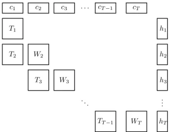
The general multi-stage stochastic linear program for a canonical probability space (Ω,A, P) can be formulated as min x1 c1x1+Eξ2 min x2 c2 (ω2)x2(ω2) +. . .+EξT min xT cT(ωT)xT(ωT) . . . s.t. T1x1 =h1 T2(ω2)x1 + W2(ω2)x2(ω2) =h2(ω2) . .. . .. .._. TT(ωT)xT−1(ωT−1) + WT(ωT)xT(ωT) =hT(ωT) lt(ωt)≤xt(ωt)≤ut(ωt) t= 1, . . . , T. (2.14)

Theξtare random vectors consisting of

(T1,t(ω), . . . , Tnt,t(ω), W1,t(ω), . . . , Wnt,t(ω), ht(ω), qt(ω))

for t= 1, . . . , T defined on a probability space (Ω,At, P) such that At⊂ A, t = 1, . . . , T and A_t⊂ A_t₊₁, t= 1, . . . , T −1. The underlying stochastic process on (Ω,A) is adapted to the filtration F ={A1, . . . ,AT}with A1 ={Ω,∅}, because the first stage contains no

(24)

c2 c1 c3 c_T₋1 c_T ._. . . . . W_T T_T −1 . . . T1 T2 W2 T3 W3 h_T h1 h2 h3

Figure 2.3. Staircase structure of program (2.14).

uncertainty. The decisions taken at stagetthus depend only on outcomes known before or at staget, they are non-anticipative with respect to the outcomes at stages greater thant.

Program (2.14) is already in staircase format, because only adjacent stages are linked via the constraints. The term staircase format follows from the graphical representation of the problem, see Figure 2.3. It may be desirable to form constraints like

Tt−1(ωt)xt−2+Tt(ωt)xt−1+Wt(ωt)xt(ωt) =ht(ωt), (2.15) to rely not just on decisions taken at staget−1 but also on those taken at earlier stages. This can be done by transforming the non-staircase constraint (2.15) into a staircase constraint with additional columns and rows as follows

xt−2= ˆxt−1 (2.16)

Tt−1(ωt)ˆxt−1+Tt(ωt)xt−1+Wt(ωt)xt(ωt) =ht(ωt). (2.17) In a first step, new stage t−1 variables are created, ˆxt−1. These are linked via the

constraint (2.16) to take the values of xt−2. The original constraint (2.15) is changed to

not include the original variablesxt−2 but the new variables ˆxt−1 instead.

It is possible to transform every problem in staircase format with this procedure. Every variable of a stage less thant−1 that is present in a non-staircase constraint at stagetneeds a staget−1 representation to replace it, see equation (2.17). Every new representation needs a constraint of type (2.16), so that the copy takes the value of the original variable. The number of variables and constraints of the transformed staircase-problem compared to the non-staircase problem is thus increased by at mostPT−2

t=1 nt·(T −1−t).

We stress here that time periods and stages can, but do not have to coincide. It is possible and due to computational considerations probably advisable that a problem with for example 24 time periods is split into six stages with four time periods belonging to each stage.

(25)

2.2.4. Basic Properties

In this section we list some basic properties of stochastic programs, in particular properties that are important for developing solution methods.

Stochastic programs can be classified according to which elements of T, W, hand q are fixed, i.e., are the same for every scenario ω. It is possible to exploit the specialized structure in a solution algorithm (Birge & Louveaux, 2011, p. 181ff). The feasibility set of the first stage K1 is defined as {x | Ax=b, x≥ 0}. The feasibility set of the second

stage K2 is defined as{x | Q(x) <∞}. Thus it is possible to reformulate the two-stage

stochastic problem given by equations (2.8)-(2.11) in terms of its feasibility sets as

z= min cx+Q(x) s.t. x∈K1∩K2.

(2.18) The recourse function Q(·, ξ) is convex. It is also polyhedral if there exists a ¯x∈K1∩K2,

i.e., Q(¯x, ξ) is finite (Shapiro et al., 2009). This is true for both continuous and discrete distributions. The expected recourse function Q(x) is polyhedral if there exists a ¯x ∈

K1 ∩K2, i.e., it has a finite value for at least one x ∈ K1. This result holds under the

assumption of finite and discrete distributions. Therefore the DEM (2.12) is a convex problem (see (Walkup & Wets, 1967) for an original proof). These results extend into the multi-stage case (Dupačová, 1995).

A program is said to have complete recourse when there exists y(ω) ≥ 0, such that

W(ω)y(ω) =t, for every vectort, t∈ Rm2_{. Thus it is guaranteed that a solution can be}

found for the second stage problem regardless of the actual value of x. A program has

relatively complete recourse if there is a y(ω) ≥0, such thatW(ω)y(ω) =h(ω)−T(ω)x

for all x ∈ K1. A program has fixed recourse, when W = W(ω),∀ω, is deterministic.

The recourse function Q(x, ω) is piecewise-linear and convex for fixed recourse problems, regardless of the distributions (Birge & Louveaux, 2011, p. 109ff).

A question that arises for every decision problem, where the introduction of uncertainty is considered, is the influence and importance of uncertainty for the problem. It has to be kept in mind that “it is extremely difficult to know if randomness is important before we have solved the problem and checked the results” (Kall & Wallace, 1994).

The measures expected value of perfect information (EVPI) and value of the stochastic solution (VSS) give some guidance towards answering the question (cf. (Birge & Louveaux, 2011, p. 163-177)). These measures are based on the solution of several different problems that we introduce first. Let

z(x, ω) = min cx+ minq(ω)y(ω)

s.t. Ax=b

T(ω)x+W(ω)y(ω) =h(ω)

x, y(ω)≥0

(2.19)

be the optimization problem associated with one particular outcomeω (Birge & Louveaux, 2011, p. 163f). Let ¯x(ω) denote the optimal solution of problem (2.19), for outcome ω.

(26)

The Here-and-Now (HN) problem is another name for the two-stage stochastic program with recourse (2.8) that we can also state as

HN = min

x Eξ[z(x, ω)]. (2.20)

The name derives from the observation that the decision maker, tasked with making a first-stage decision here and now, has to make this decision without knowing how the future will unfold, i.e., which scenario will actually take place. In contrast, the Wait-and-See (WS) problem is the hypothetical problem that the decision maker can make a first-stage decision with perfect foresight. Thus the decision maker can wait and see what happens and make the perfect decision for the revealed uncertainty. The WS problem is defined as

WS =Eξ h min x z(x, ω) i =Eξ[z(x(ω), ω)]. (2.21) Definition 2.14. The expected value of perfect information is the difference between the objective value of the Wait-and-See and the Here-and-Now problem.

The EVPI states the maximal amount you should pay a good forecaster on average so that you can adapt your first stage decision to the specific forecast. It measures how much you could gain by possessing perfect information about the future, compared with the solution of the stochastic problem. As it is usually not possible to make good forecasts all the time, the WS solution approach is not implementable in practice.

Solving the corresponding mean value problem instead of the possibly complex stochastic program is an option that could be considered by a decision maker, but that can also come with a cost. The scenario where all random parametersξ(ω) are replaced by their expectation is called the expected value scenario and is denoted with ω

EV = min

x z(x, ω), (2.22)

where ¯x(ω) denotes the optimal solution. The solution to this problem is called expected value problem solution (EV solution). This is an implementable solution because it satisfies the first-stage constraints, and it is possible to evaluate it with respect to its second stage cost by optimizing the corresponding second stage problems (2.13). This is called expected result of using the EV solution and is defined as

EEV =Eξ[z(¯x(ω), ω)]. (2.23)

Definition 2.15. The value of the stochastic solution is the difference between the objective value of the Here-and-Now problem and the expected result of using the EV solution.

The VSS measures the cost of sticking to a deterministic model if stochastic data is available. Of course, to compute the value of the stochastic solution the stochastic problem has to be built and solved first. The relation between WS, HN and EEV is as follows (Birge & Louveaux, 2011, p. 166)

(27)

This is intuitively clear, as in the WS problem the optimal first stage decision was taken for every outcome ω. This must be at least as good as the optimal first-stage decision of the stochastic program, i.e., finding a solution where all scenarios are considered together. The HN solution is at least as good as any other feasible first-stage solution for the stochastic program, in particular the EV solution, because it is optimal. The EVPI and the VSS are either equal or greater than zero. This follows from their respective definitions and relation (2.24) (Birge & Louveaux, 2011, p. 167f).

(28)

(29)

21

3. Solution Methods

In this chapter we present basic solution methods for stochastic programming problems as defined in the last chapter. To be able to do this, we introduce the notion of scenario trees in Section 3.1. The deterministic equivalent model, which can be solved by traditional LP and MIP optimization software, is then introduced in Section 3.2. We explain the main solution algorithm used in this thesis, Benders decomposition, in depth in Section 3.3. Solution methods based on an alternative decomposition approach, Lagrangean relaxation, are presented in Section 3.4. We finish this chapter with an overview about approximative solution methods and some remarks about scenario generation in Section 3.5. An introduction as well as an in-depth treatment about the different types of decomposition and direct solution methods can be found in the literature, e.g., (Birge & Louveaux, 2011; Kall & Mayer, 2010).

3.1. Scenario Tree

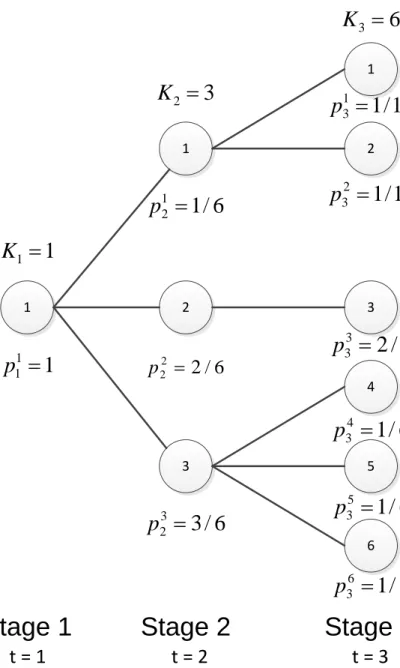
A stochastic program is specified by the deterministic structure like the number of columns and constraints, the objective function coefficients, the matrix coefficients, the right hand side and the variable bounds as well as the stochastic data. The deterministic model is also called the core model. For every scenario the stochastic data consists of coefficients that replace the respective coefficients stored in the core model. A tree structure is well suited to store the stochastic data that is different for every scenario. The scenario tree has a depth equal to the number of stages minus one. The number of leaf nodes is equal to the number of scenarios. The root node of the tree contains no stochastic data, because it represents the first stage. The probability that a certain scenario is realized is stored within the leaf node that corresponds to the scenario.

Every tree node is labeled with its staget∈1, . . . , T, withT being the number of stages, and a number from one to Kt, with Kt being the number of nodes in that stage. T also denotes the stage set {1, . . . , T}. Every node except the root node has a parent node, denoted bya(t, i), t∈1, . . . , T, i∈1, . . . , Kt. Every node except the leaf nodes has a set of child nodes, denoted by d(t, i)⊆Vt+1, t= 1, . . . , T −1, withV being the set of all nodes

of the tree and Vt the set of nodes at stage t. The path probability pit of a node is the sum of the probabilities of its child nodes. For a valid scenario tree the sum of all node probabilities at the same stage must be one. A node has also a conditional probability

cpi_t. It is defined as cpi_t = pit

pa_t₋(t,i₁), i.e., the probability of node (t,i) given its parent node (t−1, a(t, i) was chosen. For convenience, we denote by s(t, i) ⊆S the set of scenarios whose path of nodes from the root node to their respective leaf node contains the node (t, i). An example for a scenario tree for a problem with three stages and six scenarios is

(30)

1 3 1 2 6 5 4 3 2 1

Stage 1



p

3

2



K

1



K

6

3



K

(31)

3.2. Deterministic Equivalent 23

3.2. Deterministic Equivalent

The two-stage stochastic problem with recourse (2.8) can be written as a normal determin-istic LP called the determindetermin-istic equivalent model (DEM) (2.12) or extensive form (EF). The expectation in (2.12) can be replaced by a probability-weighted sum when the random variables have discrete and finite distributions, what we assume throughout this thesis. The set of scenarios is denoted withS which is also the number of scenarios. We can then formulate the DEM as the following large-scale LP

z= min x,y1_,...,yS cx+p 1_q1_y1₊ _{. . .} ₊_pS_qS_yS s.t. Ax =b T1x+ W1y1 =h1 .. . . .. ... TSx + WSyS =hS x, y1, . . . , yS ≥0. (3.1)

The LP (3.1) can be solved with state-of-the-art LP solvers, like CPLEX, Gurobi, and others. The widespread availability of modern LP solvers makes this solution approach available without resorting to special purpose software designed especially for stochastic programs. The drawback of this approach is that the special structure of stochastic programs is not used during the solution process. There are existing simplex and interior-point method (IPM) based direct solution methods that work directly with the DEM (see the introduction of Birge & Louveaux (2011, p. 222-236)). These are, to our knowledge, not implemented in commercial LP solvers.

For multi-stage stochastic programs with recourse the deterministic LP formulation is the following min c1x1+ K2 X i=1 pi₂ci₂xi₂+. . .+ KT X i=1 pi_Tci_Txi_T s.t. T1x1 =h1 Tk2 2 x1 + W2k2x k2 2 =h k2 2 k2 = 1, . . . , K2 . .. . .. .._. TkT T x a(kT,T) T−1 +W kT T x kT T =h kT T kT = 1, . . . , Kt lkt t ≤xktt ≤utkt kt= 1, . . . , Kt, t= 1, . . . , T. (3.2)

As can be seen from formulation (3.2) the corresponding columns and constraints from every scenario tree node are added to the deterministic LP. The resulting LP (3.2) is therefore a rather large scale LP which may not even be constructable due to main memory constraints.

(32)

The number of variables is equal to T X

t=1

Kt·nt,

whereas the number of constraints is equal to T X

t=1

Kt·mt.

For a two-stage problem with 1,000 columns (200 first-stage and 800 second stage) and 500 constraints (100 first-stage and 400 second-stage) and 1000 scenarios, the DEM has 800,200 columns and 400,100 constraints.

The DEM can be formulated recursively as

zi_txa_t₋(t,i₁)= min ci_txi_t+Qi_t(xi_t)

s.t. T_tixa_t₋(t,i₁)+W_tixi_t=hi_t l_ti≤xi_t≤ui_t,

(3.3)

with expected recourse function Qi t(x) = P j∈d(t,i)cp j t+1Q j t+1(xit) and Qj_t₊₁(xi_t) = min cj_t₊₁xj_t₊₁+Qj_t₊₁(xj_t₊₁) s.t. T_tj₊₁xi_t+W_tj₊₁xj_t₊₁=hj_t₊₁ lj_t₊₁≤xj_t₊_t≤uj_t₊₁, (3.4)

and the terminal condition Qj_T(·) = 0,∀j ∈ 1, . . . , KT. Problem z11(·) is equivalent to

problem (3.2), i.e., starting from the root node.

The formulations (3.1) and (3.2) are also called implicit DEM. The non-anticipativity condition is implicitly satisfied by the variables and constraints of the problem.

Another way to model the DEM is the explicit or split-variable approach. In the explicit DEM a copy of the whole deterministic model is created for every scenario, with the objective function coefficients multiplied by the respective scenario probability. This alone does not suffice, as the different copies have no link to each other, so that all the first-stage variables anticipate their respective scenario and thus yield an optimal decision for this scenario. The solution of this model yields the Wait-and-See solution. To ensure that the scenario copies of the first-stage variables do not anticipate their respective scenario, the non-anticipativity constraints

x1_t =xi_t,∀i∈S (3.5)

must be added to the formulation.

When the recourse program is a multi-stage problem, the non-anticipativity constraints must be inserted at every stage, according to the scenario tree structure. For notational convenience, we denote the set of adjacent pairs of child nodes of a node (t, i) withN(t, i) =

(33)

3.3. Benders Decomposition 25

{(s1, s2)|s1, s2 ∈s(t, i)∧s1+ 1 =s2}. For every node of the tree, except the leaf nodes,

the following constraints are added to the explicit DEM formulation

xs1

t =xst2, ∀t∈ {1, . . . , T −1},∀i∈ {1, . . . , Kt},∀(s1, s2)∈N(t, i). (3.6)

They ensure that all decisions belonging to nodes with the same parent node take the same value. Of course it is also possible to model these constraints differently, e.g., by using one scenario as the reference scenario (Fourer & Lopes, 2006), as we did for the two-stage case.

For the exemplary scenario tree in Figure 3.1, the following non-anticipativity constraints given by equation (3.6) would be present in the explicit DEM

x1₁ =x2₁, x2₁ =x3₁, x3₁ =x4₁, x4₁ =x5₁, x5₁ =x6₁ x1₂=x2₂, x4₂=x5₂, x5₂=x6₂.

The explicit DEM formulation

min T X t=1 S X s=1 pscstxst s.t. T₁sxs₁ =hs₁ s= 1, . . . , S T₂sxs₁ +W₂sxs₂ =hs₂ s= 1, . . . , S . .. . .. .._. T_Tsxs_T₋₁ + W_Tsxs_T =hs_T s= 1, . . . , S xs1 t =xst2, t= 1, . . . , T −1, i= 1, . . . , Kt,∀(s1, s2)∈N(t, i) ls_t ≤xs_t ≤us_t s= 1, . . . , S, t= 1, . . . , T, (3.7)

has even more constraints and variables than the implicit DEM. The number of variables is equal to S T X t=1 nt, whereas the number of constraints is equal to

T X t=1 Kt X i=1 (|s(t, i)| −1) +S T X t=1 mt.

3.3. Benders Decomposition

A well known solution method for two-stage stochastic linear programs with recourse is the L-shaped method by (Van Slyke & Wets, 1969), an adaption of Benders decomposition (Benders, 1962) to stochastic problems. The main idea is to approximate the recourse function by an iteratively refined outer linearization via cutting planes. It is also possible to perform an inner linearization via Dantzig-Wolfe decomposition (Dantzig & Wolfe, 1961) that works on the dual problem (see e.g., (Birge & Louveaux, 2011, p. 237-242) for an introduction).

(34)

The problem is decomposed by stage into a first-stage master problem and several second-stage subproblems. The first-stage master problem approximates the recourse function with a linear term and delivers an optimal solution for the current approximation. The second-stage subproblems evaluate the chosen first-stage solution for every scenario. With the dual information, the linear approximation is refined and the master problem is resolved. This process repeats until the original problem is solved to optimality. The following detailed description of the Bender’s decomposition method applied to stochastic program is based on the work of Freund (2004). It explains the multi-cut form (Birge & Louveaux, 1988) of the algorithm.

The algorithm is used to solve the two-stage stochastic problems with recourse (2.8). The deterministic equivalent formulation (3.1) of the problem can also be written as problem (2.12) with the second-stage problems (2.13)Q(x, s), withs∈S. We denote the dual of

problemQ(x, s) as D(x, s)

D(x, s) :=z(x, s) = max πs(hs−Tsx)

s.t. (Ws)Tπs≤qs. (3.8)

The feasible region ofD(·, s) is the set

D_s:=nπs |(Ws)Tπs≤qso,

which is independent of x. If the polyhedron is full-dimensional, the extreme points and extreme rays of the feasible regionD_s can be enumerated with πs,1, . . . , πs,Is _{as extreme}

points and rs,1, . . . , rs,Js _{as extreme rays (Freund, 2004). If the polyhedron is not full}

dimensional, it does not have extreme points, but rather “extreme hyperplanes”. The polyhedron can still be finitely generated by a set of vectors, where each vector belongs to a different minimal face of Ds, and a set of its extreme rays, as described by Equation (2.7) in Section 2.1.

By the addition of a slack vector to the constraint (Ws₎T_pts _≤ _qs_{, two finite sets of} vectors can be defined that fulfill the same goal as the sets of extreme points and extreme rays, namely that they are finite and that the polyhedron can be decomposed into these two sets according to the Minkowski-Weyl decomposition theorem (2.13). The two sets are the set of basic feasible solution of D(·, s) and the set of feasible rays composed of minimal dependent sets of the matrix columns of WTI, see (Zverovich et al., 2012) for details. As the LP solver converts the problem internally into a full-dimensional problem by the addition of slack variables (e.g., (Maros, 2003, p. 4-18)), we continue with the assumption of the full-dimensional case.

If problemD(x, s) is solved, it can either be unbounded or optimal. If the problem is optimal, we get an extreme point of the feasible region as a solution ¯πs=πs,i, i∈ {1, . . . , Is}. As this solution is optimal it holds that

z(x, s) = ¯πs(hs−Tsx) = max k=1,...,Is

(35)

3.3. Benders Decomposition 27

and the solution value z(x, s) is thus greater equal than

πs,i(hs−Tsx), i∈ {1, . . . , Is}.

If the problem is unbounded, the solver returns an extreme ray ¯rs=rs,j, j∈ {1, . . . , Js}. The solution valuezsis therefore∞and thus ¯rs(hs−Tsx)>0. As long as it holds for any extreme ray rs,j _that_rs,j₍_hs₋_Ts_x₎_>_{0, the second-stage problem} _D₍_{x, s}_{) is unbounded.} Therefore the solution x must be chosen differently to be feasible, as h and T are fixed and determined by the scenarios.

With these two observations we can rewriteD(x, s) in terms of the extreme points and extreme rays of its feasible region Ds as

D2(x, s) :=z(x, s) = min zs

s.t. πs,i(hs−Tsx)≤zs i= 1, . . . , Is

rs,j(hs−Tsx)≤0 j= 1, . . . , Js.

(3.9)

A solution ¯xthat would lead to problemD(x, s) being unbounded is not feasible for problem

D2(x, s). Thus D(¯x, s) =∞=D2(¯x, s) as D(·, s) is a maximization problem. Therefore we can replaceQ(x, s) in problem (2.12) byD2(x, s). If we also replace the expectation by the probability weighted sum, we can write this problem, also known as the full master problem (FMP) (Freund, 2004), as z= min x,z1_,...,zS c T_x₊ S X s=1 pszs s.t. Ax=b x≥0 (3.10) πs,i(hs−Tsx) ≤zs i= 1, . . . , Is, s= 1, . . . , S rs,j(hs−Tsx) ≤0 j= 1, . . . , Js, s= 1, . . . , S.

If we compare this reformulation with problem (3.1), we see that we removed the second stage variables ys and the corresponding constraints from the problem, we addedS many scalar variables, and a really huge number of constraints. This approach is generally not computationally feasible due to the large number of extreme points and extreme rays of the feasible regions of every second-stage dual subproblem and the resulting number of constraints. The idea is to start with a restricted master problem without any additional constraints and generate the missing constraints when we notice that a not yet added

(36)

constraint was violated. The restricted master problem at a given iterationitis formulated like this zit= min x,z1_,...,zS c T_x₊ S X s=1 pszs s.t. Ax=b x≥0 (3.11)

πs,i(hs−Tsx) ≤zs for someiand s rs,j(hs−Tsx) ≤0 for some iand s.

A solution to problem (3.11) gives us an optimal first-stage solution ¯x,z¯1, . . . ,z¯S. The solution value zit is a lower bound to the optimal solution value z of the FMP, as the

RM Pit misses some constraints that the FMP already has. We now need to check if the given solution is optimal for the FMP. We do this by solving problem (3.8) for ¯xand every

s. As already described above, ifD(¯x, s) has an optimal solution we get an extreme point

πs,i. If D(¯x, s) is unbounded, we get an extreme ray rs,j. If it holds that the objective function value of Q(¯x, s) = D(¯x, s), namely z(¯x, s) is greater than the approximating variable ¯zs

z(¯x, s) =πs,i(hs−Tsx¯)>z¯s,

than the solution ¯x,z¯s violated the constraintπs,i(hs−Tsx)≤zs, and this constraint is then added to RM Pit. This constraint is called optimality cut and is usually rearranged to take the form

πs,iTsx+zs≥πs,ihs.

IfD(¯x, s) is unbounded, we have an extreme rayrs,j. The inequalityrs,j(hs−Tsx)>0 holds for this extreme ray. The constraintrs,j(hs−Tsx)≤0 is therefore violated and is added toRM Pit. This constraint is called feasibility cut.

If all the problems D(¯x, s) have a finite optimal solution, it is possible to compute an upper bound for the original problem (2.12) because every feasible solution ¯x,y¯1, . . . ,y¯S is always greater or equal than the optimal solution. The objective function value of the solution x can be computed as cx+PS

s=1psqsys. If this value is lower than the current

upper bound, the upper bound can be updated and the solution ¯x,y¯1, . . . ,y¯S can be stored as the incumbent solution. This is repeated until the stopping condition is met. There are three stopping conditions that can be checked. We can stop the algorithm, if no violated constraint could be found, i.e., no cut was added to the RM Pit. This means that the found solution is optimal for the FMP and therefore for the original problem. In theory this stopping condition would suffice, but because of numerical inaccuracies in real world computations, it might not be possible to achieve this condition. The algorithm can also be stopped if the gap between the upper and lower bound, ∆ = U B −LB, is smaller than a small tolerance optimality.1 The third stopping criterion is not an absolute but a relative stopping criterion. When the fraction _|_LB|U B_|₊₁₀−LB−10| is smaller than anoptimality, the

1