A Probabilistic Prolog and its Applications

(1)

Arenberg Doctoral School of Science, Engineering & Technology Faculty of Engineering

Department of Computer Science

A Probabilistic Prolog and its Applications

Angelika Kimmig

Dissertation presented in partial fulfillment of the requirements for the degree of Doctor

in Engineering

(2)

(3)

A Probabilistic Prolog and its Applications

Angelika Kimmig

Jury: Dissertation presented in partial

Prof. Dr. ir. Ann Haegemans, president fulfillment of the requirements for Prof. Dr. Luc De Raedt, promotor the degree of Doctor

Prof. Dr. ir. Maurice Bruynooghe in Engineering Prof. Dr. ir. Erik Duval

Prof. Dr. ir. Gerda Janssens Prof. Dr. Taisuke Sato

(Tokyo Institute of Technology, Japan) Prof. Dr. V´ıtor Santos Costa

(Universidade do Porto, Portugal)

(4)

Alle rechten voorbehouden. Niets uit deze uitgave mag worden vermenigvuldigd en/of openbaar gemaakt worden door middel van druk, fotocopie, microfilm, elektronisch of op welke andere wĳze ook zonder voorafgaande schriftelĳke toestemming van de uitgever.

D/2010/7515/121 ISBN 978-94-6018-282-2

(5)

Abstract

One of the key challenges in artificial intelligence is the integration of machine learning, relational knowledge representation languages and reasoning under uncertainty. Given its multi-disciplinary nature, this topic has been approached from different angles, leading to a very active research area known as probabilistic logic learning or statistical relational learning.

Motivated by the need for a probabilistic logic language with an implementation that supports reasoning in large networks of uncertain links, as they arise for instance when integrating information from various databases, this thesis introduces ProbLog, a simple extension of the logic programming language Prolog with independent random variables in the form of probabilistic facts. While ProbLog shares its distribution semantics with other approaches developed in the field of probabilistic logic learning, its implementation has been the first to allow for scalable inference in networks of probabilistic links. This is due to the use of advanced data structures that make it possible to base probabilistic inference on proofs or explanations even if those are not mutually exclusive in terms of the possible worlds they cover. As a general purpose probabilistic logic programming language, ProbLog provides a framework for lifting relational learning approaches to the probabilistic context. We apply this methodology to obtain three new probabilistic relational learning techniques. The first one, theory compression, is a form of theory revision that reduces a ProbLog program to a given maximum size by deleting probabilistic facts, using example queries that should or should not be provable with high probability as a guideline. The second example, probabilistic explanation based learning, naturally extends explanation based learning to a probabilistic setting by choosing the most likely proof of an example for generalization. The third approach, probabilistic query mining, combines multi-relational data mining with scoring functions based on probabilistic databases. The latter two techniques are also used to illustrate the application of ProbLog as a framework for reasoning by analogy, where the goal is to identify examples with a high probability of being covered by logical queries that also assign high probability to given training examples. While these approaches all rely on ProbLog programs with known probability labels, we

(6)

ii

also introduce a parameter estimation technique for ProbLog that determines those labels based on examples in the form of queries or proofs augmented with desired probabilities. Throughout the thesis, we experimentally evaluate the methods we develop in the context of a large network of uncertain information gathered from biological databases.

While the main focus of this thesis lies on ProbLog and its applications, we also contribute a second framework calledωProbLog, which generalizes ProbLog to

weight labels from an arbitrary commutative semiring. We introduce inference algorithms that calculate weights of derived queries, showing that the ideas underlying the ProbLog system carry over to more general types of weights.

(7)

Acknowledgements

Working on this Ph.D. has been a fun and exciting journey that would not have been possible without the support of many people. First of all, I’d like to thank my supervisor Luc De Raedt. His enthusiasm – together with that of Kristian Kersting – has guided me from that first seminar on probabilistic logic learning via my diploma thesis right into this Ph.D. adventure. I sometimes still wonder how exactly they managed to get me interested in probabilities. . .But they certainly did!

From the beginning, Luc has been a true expert in both motivating and challenging me with a single word or question. I have learned a lot from working with him, often without even realizing it. Moreover, he has also given me the opportunity to explore a new country, and to practice juggling with several (natural) languages on a daily basis. Bedankt, Luc!

Besides Luc, I’ve had the chance to work with many others, both within the ML groups in Freiburg and Leuven and beyond. Back in Freiburg, Hannu Toivonen, Kristian Kersting and Kate Revoredo have made the initial months a lot easier than I would have imagined, while Ralf Wimmer has introduced me to the practical side of binary decision diagrams. Later on, the first floor PLL island in Leuven has been a great place to work, with the ProbLog and Prolog experts Bernd Gutmann and Theofrastos Mantadelis, and with Daan Fierens quietly ensuring that the three of us wouldn’t forget the rest of PLL – and keep at least some of our discussions and bug hunting fights to a bearable noise level ;-) This thesis would not have been possible without the Prolog expertise from both Leuven and Porto. I am grateful to V´ıtor Santos Costa, Ricardo Rocha, Bart Demoen and Gerda Janssens for joining our team. Maurice Bruynooghe and Joost Vennekens never lost their patience in explaining me the fine details of semantics. I also thank Dimitar Shterionov for letting one of my ideas take over his master thesis topic, and Fabrizio Costa for challenging me with a constant stream of ideas on how to use ProbLog. Ingo Thon and Guy Van den Broeck have provided new insights in many discussions. Finally, I’d also like to thank all the other members of ML and DTAI for their comments on my work, and for the company during conference trips and Alma lunches. Dat laatste groepje will ik ook bedanken voor de dagelĳkse lessen Nederlands. I further thank Hannu, V´ıtor, and David Page and Jude Shavlik for welcoming me as a

(8)

iv

visitor in their groups in Helsinki, Porto, and Madison.

This thesis builds on the work of many others, both in machine learning and logic programming. I am lucky to have four of these experts, Taisuke Sato, V´ıtor Santos Costa, Maurice Bruynooghe, and Gerda Janssens, serving on my Ph.D. committee, and I’d like to thank them for their excellent feedback on my work. I also thank Erik Duval for enriching the committee with a different perspective, and Ann Haegemans for chairing my defense.

I gratefully acknowledge the financial support received for the work performed during this thesis from the European Union FP6-508861 project on “Applications of Probabilistic Inductive Logic Programming II”, the GOA/08/008 Probabilistic Logic Learning, and the research foundation Flanders (FWO-Vlaanderen). Of course, there’s a lot more to life than 0s and 1s, and even more than all the probabilities in between. Beyond work, I’d like to especially thank Bettina, Ralf, H¨ulya and Konrad for many discussions during extended teatimes and countless walks (random and planned, back home and all over Europe), and simply for their friendship throughout the years. I also thank my orchestra colleagues in both Freiburg and Leuven for regularly dragging me off my computer with evenings and weekends full of music, hard work and great fun. Finally and most importantly, I want to thank my parents and my sister for their unconditional support. Danke, daß Ihr immer f¨ur mich da seid!

Angelika Kimmig Leuven, November 2010

(9)

4.3 Implementation . . . 70 4.3.1 Labeled Facts . . . 72 4.3.2 Explanations . . . 73 4.3.3 Sets of Explanations . . . 73 4.3.4 From DNFs to BDDs . . . 77 4.3.5 Program Sampling . . . 78 4.3.6 DNF Sampling . . . 80 4.4 Experiments . . . 81 4.5 Related Work . . . 88 4.6 Conclusions . . . 89 Conclusions Part I 91

Intermezzo

93

5 ωProbLog 95 5.1 A Generalized View on ProbLog Inference . . . 96

5.2 From ProbLog toωProbLog . . . 100

5.3 Related Work . . . 108

II

BDD-based Learning

111

Outline Part II 113 6 Theory Compression 115 6.1 Compressing ProbLog Theories . . . 116

(12)

viii CONTENTS

6.3 Experiments . . . 120

6.3.1 Data . . . 120

6.3.2 Implementation . . . 122

6.3.3 Quality of ProbLog Theory Compression . . . 122

6.3.4 Complexity of ProbLog Theory Compression . . . 127

7 Parameter Learning 131 7.1 Related Work . . . 132

7.2 Parameter Learning in Probabilistic Databases . . . 134

7.3 Gradient of the Mean Squared Error . . . 136

7.4 Parameter Learning Using BDDs . . . 137

Conclusions Part II 145

III

Reasoning by Analogy

147

Outline Part III 149 8 Inductive and Deductive Probabilistic Explanation Based Learning 151 8.1 Explanation-based Analogy in Probabilistic Logic . . . 152

8.2 Background: Constructing Explanations . . . 154

8.2.1 Explanation Based Learning . . . 154

8.2.2 Query Mining . . . 156

8.2.3 Deductive and Inductive EBL . . . 164

(13)

CONTENTS ix

8.3.1 Probabilistic Explanation Based Learning . . . 165

8.3.2 Probabilistic Local Query Mining . . . 167

8.4 Implementation . . . 170

8.5.1 Probabilistic EBL . . . 171

8.5.2 Probabilistic Query Mining . . . 174

Conclusions Part III 181

Finale

183

9 Summary and Future Work 185

Appendix

191

A Biomine Datasets 193

Bibliography 195

Publication List 207

(14)

(15)

List of Figures

2.1 SLD-tree forpath(a,b) . . . 12

2.2 Bayesian network . . . 19

2.3 Full binary decision tree and BDD forx∨(y∧z) . . . 20

2.4 BDD ordering example . . . 22

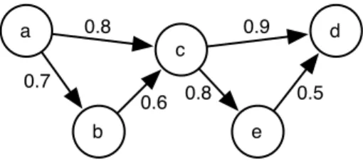
3.1 Probabilistic graph example . . . 30

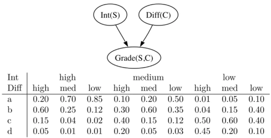
3.2 Fragment of school example . . . 46

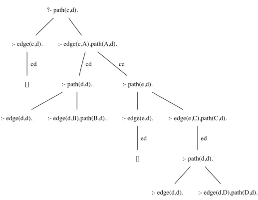
4.1 SLD-tree of Example 3.1 . . . 57

4.2 Binary decision diagram forcd∨(ce∧ed) . . . 62

4.3 Example of possible worlds in DNF sampling . . . 68

4.4 ProbLog implementation . . . 71

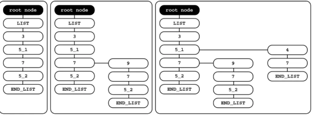
4.5 Using tries to store explanations . . . 75

4.6 Example of nested tries . . . 76

4.7 Recursive node merging forpath(a,d) . . . 79

5.1 BDD of Example 5.5 . . . 105

6.1 Theory compression example . . . 118

6.2 BDDs illustrating fact deletion . . . 121

6.3 Evolvement of log-likelihood . . . 122

(16)

xii LIST OF FIGURES

6.4 Evolvement of log-likelihood with artificially implanted edges . . . 123

6.5 Evolvement of log-likelihoods in random runs . . . 125

6.6 Effect of compression on log-likelihoods . . . 126

6.7 Runtimes . . . 127

7.1 Results√M SEtest . . . 141

7.2 ResultsM ADfacts. . . 142

7.3 Results for varyingk . . . 142

7.4 Results for learning from proofs and queries . . . 143

8.1 SLD-trees for Examples 8.2 and 8.12 . . . 156

8.2 Proof trees for Example 8.2 . . . 157

8.3 Explanations forpath(A,B) . . . 171

(17)

List of Tables

4.1 k-probability on_Small . . . 83

4.2 Bounded approximation onSmall . . . 83

4.3 Program sampling onSmall . . . 84

4.4 k-probability onMedium . . . 84

4.5 Program sampling using memopath/3onMedium. . . 85

4.6 k-probability on_Biomine . . . 86

4.7 Program sampling using memopath/3onBiomine . . . 86

4.8 Program sampling using lenpath/4onBiomine . . . 87

4.9 DNF sampling usinglenpath/4on_Biomine . . . 87

5.1 A unifying view on ProbLog inference . . . 98

5.2 Examples ofωProbLog semirings . . . 106

8.1 Counts onid+ _and_id− _and_ψ_{-values . . . 163}

8.2 Aggregates onid+ andid− . . . 169

8.3 Queries refined after the first level of query mining . . . 169

8.4 Graph characteristics . . . 173

8.5 Reasoning by analogy on different graphs . . . 173

8.6 Fraction of successfully terminated cases . . . 175

8.7 Overall results of reasoning by analogy using best query . . . 176

(18)

xiv LIST OF TABLES

8.8 Quality of top ranked examples . . . 176 8.9 Mining onAlzheimer4 . . . 177 A.1 Biomine datasets . . . 194

(19)

List of Algorithms

4.1 ResolutionStep . . . 58 4.2 Resolve . . . 58 4.3 ResolveThreshold . . . 59 4.4 BestProb . . . 59 4.5 Probability . . . 61 4.6 Bounds . . . 64 4.7 ProgramSampling . . . 66 4.8 DnfSampling . . . 69 4.9 RecursiveNodeMerging . . . 77 5.1 Map . . . 99 5.2 ExplanationWeight . . . 103 5.3 InterpretationWeight . . . 104 5.4 InterpretationWeightBdd . . . 104 5.5 InterpretationWeightBddGeneral . . . 106 6.1 Compress . . . 119 7.1 Gradient . . . 137 7.2 GradientDescent . . . 138 8.1 SelectedQueries. . . 160 8.2 CorrelatedQueries . . . 162 xv

(20)

(21)

List of Symbols

T ProbLog program

BK Background knowledge

pi::fi Probabilistic fact

bi Propositional variable corresponding topi::fi

FT _{Set of groundings of probabilistic facts in}_T

LT FT without probability labels I Partial interpretation ofLT I1 Set of facts assigned true inI I0 _{Set of facts assigned false in}_I

I? _{Set of facts with unassigned truth value in}_I

ComplT₍_I_{) Set of complete interpretations of}_LT _extending_I

PT₍_I₎ _{Probability of interpretation}_I _{given by program}_T

MI(T) Least Herbrand model ofLT ∪BK extendingI

I|=T q Isupports queryq

E Explanation

ExplT(q) Set of explanations of queryqin T

(22)

xviii List of Symbols

DT_s(q) DNF encoding of all interpretations supporting queryq DTx(q) DNF encoding ofExplT(q)

DT

xs(q) Syntactical extension ofDxT(q) to complete interpretations

PT x(q) Explanation probability PT s (q) Success probability PT k (q) k-probability ST x(q) Sum of probabilities PT M AP(q) MAP probability

(23)

Overture

(24)

(25)

Chapter 1

Introduction

Building computer programs that solve specific types of tasks considered to require intelligence is the driving force behind current progress in the field of artificial intelligence. While the notion of intelligence is difficult to grasp in formal terms, from the point of view of solving a certain type of problem or performing a certain task, it involves abilities such as dealing with possibly large amounts of data of various types and formats as well as general knowledge about the domain, identifying those pieces of information relevant for the specific problem instance at hand, coping with situations that have not been foreseen at the time of programming, and taking into account uncertainty both in the available knowledge and in the reasoning process.

A suitable knowledge representation language and corresponding reasoning

mechanisms are key components to achieve those abilities. A prominent choice are subsets of first order logic, most notably definite clause logic. Such languages make it easy to integrate heterogeneous types of knowledge about specific entities, ranging from simple attribute-value descriptions to structured or interrelated data, with general, abstract knowledge about the domain of interest. Other relational languages are widely used as well. For instance, graph languages are a popular choice for collections of binary relations such as links between web pages, citations between scientific papers, or relations between persons in social networks. Such relational languages can conveniently be emulated in definite clause logic, making it an interesting framework for general language comparisons as well. From a practical perspective, definite clause logic forms the backbone oflogic programming[Lloyd, 1989], a field that has developed optimized algorithms and implemented corresponding reasoning systems. Inference is typically based on a form of backward chaining from a given query, which naturally focuses on the relevant parts of the database. For more details, we refer to Section 2.1.

(26)

4 INTRODUCTION

While logic programming primarily follows a deductive approach to reasoning, where only explicitly available information is used, machine learning adds an

inductivecomponent, where regularities in the available data are made explicit and transferred to other instances of the same type. Formally, a computer program is said to learn if it improves its performance with respect to a class of tasks based on experience [Mitchell, 1997]. Learning often aims at obtaining a model of the data or of some process that could have generated the data. Such a model can then be used for classification of new data points, which in turn provides additional information for problem solving. Alternatively, the model itself can be analyzed to obtain new insights into the domain. This is especially true if learning uses a language understandable for human experts, such as association rules or logical theories. Finding association rules or other types of local patterns in data is also studied in the field ofdata miningas part of the process of knowledge discovery in databases [Fayyad et al., 1996]. While both machine learning and data mining traditionally worked with propositional or attribute-value data, the need to deal with more complex structured or relational data has lead to the growing subfield known as inductive logic programming (ILP) [Muggleton and De Raedt, 1994], multi-relational data mining [Dˇzeroski and Lavraˇc, 2001], or logical and relational learning [De Raedt, 2008]. Many approaches developed in this field again build on the computational framework of logic programming and definite clause logic. While logical and relational languages are rich knowledge representation tools, they are not able to explicitly deal with the uncertainty inherent in real world data and problems, whether stemming from imprecision in the data collection process or contradictory information from different sources, or simply from the fact that abstract rules often hold in general, but can have exceptions. To deal with this type of problems, relational languages need to be integrated with some mechanism to cope with uncertainty based on for instance statistical models or probability theory. A variety of such approaches and corresponding learning techniques have been developed in the field known as probabilistic logic learning (PLL) [De Raedt and Kersting, 2003], statistical relational learning (SRL) [Getoor and Taskar, 2007] or probabilistic inductive logic programming (PILP) [De Raedt and Kersting, 2004; De Raedt et al., 2008a]; we refer to Section 2.3 for a brief overview. While these languages are very expressive in general, their implementations often impose restrictions to increase efficiency, or are tailored towards specific tasks, which, despite the wide range of languages, can make it difficult to find one that is directly usable for a new task at hand.

Probabilistic logic languages originating from the areas of machine learning and knowledge representation often focus on themodeling aspect of the underlying logical language, even in the case of definite clause languages close to (pure) Prolog. Recently, theprogramming view on such languages is receiving increased attention. Indeed, with probabilistic semantics rooted in the semantics of logic programming and Prolog, as defined for instance by Sato’s distribution

(27)

INTRODUCTION 5

semantics [Sato, 1995], languages such as PRISM [Sato and Kameya, 2001] are general programming languages adapted for probabilistic purposes. They have the potential to extend probabilistic definite clause languages similarly to how Prolog as a programming language extends its core definite clause language. Clearly, probabilistic programming is not restricted to logic programming, but similar ideas emerge in other areas, including for instance functional languages such as IBAL [Pfeffer, 2001] and Church [Goodman et al., 2008], or Figaro [Pfeffer, 2009], which combines functional and object-oriented aspects. Such languages typically calculate point probabilities; however, probability intervals have been investigated as well, for instance in probabilistic logic programming as defined by Ng and Subrahmanian [1992].

Thesis Contributions and Roadmap

This thesis develops and implements a probabilistic logic programming language that can represent a broad range of problems, including link mining tasks in large networks of uncertain relationships. Apart from effective and efficient reasoning algorithms, the resulting system also provides a general framework for lifting traditional ILP tasks to probabilistic ILP, as will be illustrated for a number of techniques. Link mining and reasoning in large biological networks are used as a testbed for all approaches discussed throughout the thesis.

Sato’s distribution semantics [Sato, 1995] provides a thorough theoretical basis for extending logic programming or definite clause logic with independent probabilistic facts. Its basic idea is to use logic programs to model discrete probability distributions over logical interpretations. However, existing PLL systems based on the distribution semantics, such as the ones for PRISM [Sato and Kameya, 2001] and ICL [Poole, 2000], have practical limitations. The PRISM system imposes additional requirements on programs to simplify inference. Specifically, each logical interpretation can only contain one of a set of so-called observable ground atoms with a single proof or explanation. While the ICL implementation Ailog2 does not rely on such additional assumptions, it does not scale very well. In particular, these limitations prevent the application of those systems in the context of mining and analyzing large probabilistic networks, which can naturally be represented – and complemented with background knowledge – in probabilistic logic. An example of such a network is Sevon’s Biomine network [Sevon et al., 2006] which contains relationships between various types of biological objects, such as genes, proteins, tissues, organisms, biological processes, and molecular functions. These relationships have been extracted from large public databases such as Ensembl and NCBI Entrez, where weights have been added to reflect uncertainty. Mining this type of data has been identified as an important and challenging task, see e.g. [Perez-Iratxeta et al., 2002], but few tools are available to support this process.

(28)

6 INTRODUCTION

The need to overcome the above mentioned limitations of probabilistic logic languages for biological network mining has motivated our work on ProbLog, a probabilistic logic programming language based on the distribution semantics. Our inference algorithms for ProbLog are based on advanced data structures to enable probability calculation without additional assumptions. The implementation of these algorithms uses state-of-the-art Prolog technology as offered by YAP-Prolog, which drastically improves scalability in the network setting. However, as ProbLog is a general probabilistic logic programming language, it can not only be used for mining large networks, but also offers a framework to transfer techniques from inductive logic programming (ILP) to the probabilistic setting. Such probabilistic ILP approaches broaden the notion of logical coverage into a gradual one, where probabilities quantify the degree of truth. As these techniques typically require the evaluation of large amounts of queries, efficient inference methods as provided by ProbLog are crucial for their successful application. In this thesis, we employ ProbLog to develop a number of PILP techniques which eitherimproveprobabilistic theories with respect to given examples, or exploit probabilistic information to

reason by analogy. Furthermore, we show that ProbLog inference can directly be adapted to domains with different types of fact labels, such as cost networks or weighted propositional logic, resulting in the introduction of ωProbLog, which

generalizes ProbLog’s probability labels to labels from an arbitrary commutative semiring.

The core of this thesis is divided into three main parts, discussing the ProbLog language and its implementation, machine learning techniques that improve ProbLog theories based on examples, and methods to reason by analogy using ProbLog, respectively. In all parts, we will use the Biomine network for experiments demonstrating the applicability of ProbLog techniques in real-world collections of probabilistic data. An intermezzo after the first part takes a step back and investigates the question of how to apply ProbLog techniques if probability labels are replaced by other types of weights. In the following, we give a brief overview of the main contributions of each part.

Part Iis devoted to ProbLog’s syntax and semantics, inference algorithms, and implementation. InChapter 3, we lay the foundations by introducing ProbLog, an extension of Prolog whereprobabilistic factsare used to define a distribution over canonical models of logic programs, which serves as the basis to define the success probability of logical atoms or queries. The semantics of ProbLog is not new: it is an instance of Sato’s well-known distribution semantics. However, in contrast to many other languages based on this semantics, ProbLog is targeted at efficient and scalable inference without making any assumptions beyond independence of basic random variables. To this aim,Chapter 4contributes various algorithms for exact and approximate inference in ProbLog. Our implementation of ProbLog on top of the state-of-the-art YAP-Prolog system uses binary decision diagrams (BDDs) to efficiently calculate probabilities. To the best of our knowledge, ProbLog has been

(29)

INTRODUCTION 7

the first PLL system using BDDs, an approach that currently receives increasing attention in the fields of probabilistic logic learning and probabilistic databases, cf. for instance [Riguzzi, 2007; Ishihata et al., 2008; Olteanu and Huang, 2008; Thon et al., 2008; Riguzzi, 2009]. The techniques exploited in our implementation enable the use of ProbLog to effectively query Sevon’s Biomine network [Sevon et al., 2006] containing about 1,000,000 nodes and 6,000,000 edges. ProbLog is included in the publicly available stable version of YAP.1_{Part I is based mainly on}

the following publications:

L. De Raedt, A. Kimmig, and H. Toivonen. ProbLog: A probabilistic Prolog and its application in link discovery, in Proceedings of the 20th International Joint Conference on Artificial Intelligence (ĲCAI–2007), Hyderabad, India, 2007.

A. Kimmig, V. Santos Costa, R. Rocha, B. Demoen, and L. De Raedt.

On the efficient execution of ProbLog programs, in Proceedings of the 24th International Conference on Logic Programming (ICLP–2008), Udine, Italy, 2008.

A. Kimmig, B. Demoen, L. De Raedt, V. Santos Costa, and R. Rocha.

On the Implementation of the Probabilistic Logic Programming Language ProbLog, Theory and Practice of Logic Programming, accepted, 2010. Before moving on to learning and mining techniques for ProbLog, theIntermezzo inChapter 5introducesωProbLog, a generalization of ProbLog where probability

labels are replaced by semiring weight labels, together with a set of algorithms that correspondingly extend ProbLog’s inference algorithms.

InPart II, we discuss machine learning techniques that improve ProbLog programs with respect to a set of example queries. Chapter 6introduces the task oftheory compression, where the size of a ProbLog database is reduced based on queries that should or should not have a high success probability. It is a form of theory revision where the only operation allowed is the deletion of probabilistic facts, which is evaluated in terms of the effect on the probabilities of the example queries. While deleting a fact can also be seen as setting its probability to 0,

parameter learning as discussed inChapter 7allows for arbitrary fine-tuning of probabilities. In this regard, we introduce a novel setting for parameter learning in probabilistic databases, which differs from the common setting of parameter learning for generative models, as such databases do not define a distribution over example queries. We provide a parameter estimation algorithm based on a gradient descent method, where examples are labeled with their desired probability. The approach integrates learning from entailment and learning from proofs, as examples can be provided in the form of both queries and proofs. The methods discussed in

1

(30)

8 INTRODUCTION

this part directly exploit the BDDs generated by ProbLog’s inference engine to efficiently evaluate the effect of possible changes. The material presented in Part II has been published in the following main articles:

L. De Raedt, K. Kersting, A. Kimmig, K. Revoredo, and H. Toivonen.

Compressing probabilistic Prolog programs, Machine learning, 70(2-3), 2008.

B. Gutmann, A. Kimmig, K. Kersting, and L. De Raedt. Parameter learning in probabilistic databases: A least squares approach, in Proceedings of the 19th European Conference on Machine Learning (ECML–2008), Antwerp, Belgium, 2008.

Part IIIfocuses on explanation learning for reasoning by analogy. Explanation learning is concerned with identifying an abstract explanation with maximal probability on given example queries. Such an explanation can then be used to retrieve analogous examples and to rank them by probability. InChapter 8, we introduce two alternative approaches to explanation learning. In probabilistic explanation based learning (PEBL), the problem of multiple explanations as encountered in classical explanation based learning is resolved by choosing the most likely explanation. PEBL deductively constructs explanations by generalizing the logical structure of the most likely proofs of example queries in a domain theory defining a target predicate. Probabilistic local query mining extends existing multi-relational data mining techniques to probabilistic databases. It thus follows an inductive approach, where the pattern language is defined by means of a language bias and the search for patterns is structured using a refinement operator. Furthermore, negative examples can be incorporated in the score to find correlated patterns. The work presented in Part III has been published previously in:

A. Kimmig, L. De Raedt, and H. Toivonen. Probabilistic explanation based learning, in Proceedings of the 18th European Conference on Machine Learning (ECML–2007), Warsaw, Poland, 2007. Winner of the ECML Best Paper Award (592 submissions).

A. Kimmig and L. De Raedt. Local query mining in a probabilistic Prolog, in Proceedings of the 21st International Joint Conference on Artificial Intelligence (ĲCAI–2009), Pasadena, California, USA, 2009. Finally, some of the work performed during my Ph.D. research has not been included in this text, but will be briefly summarized in Chapter 9 in the context of related future work; more details can be found in [Kimmig and Costa, 2010] and [Bruynooghe et al., 2010].

(31)

Chapter 2

Foundations

In this chapter, we review a number of important concepts used throughout this thesis. We start in Section 2.1 with logic programming. Section 2.2 presents Sato’s distribution semantics, which extends logic programming with probabilistic facts. Section 2.3 provides a brief overview of probabilistic logic learning. Binary decision diagrams as introduced in Section 2.4 are one of the key ingredients of our efficient implementation of ProbLog. Finally, in Section 2.5, we briefly discuss Sevon’s Biomine network as an example application to be used in our experiments.

2.1 Logic Programming

In this section, we will briefly review the basic concepts of logic programming. For more details, we refer to [Lloyd, 1989; Flach, 1994]. We use Prolog’s notational conventions, i.e. variable names start with an upper case letter, names of all other syntactic entities with lower case letters.

Example 2.1 Using successor notation, the following program defines the set of natural numbers as well as a relation smalleramong them.

nat(0).

nat(s(X)) :− nat(X).

smaller(0,s(X)).

smaller(s(X),s(Y)) :− smaller(X,Y).

(32)

10 FOUNDATIONS

In the example,0is the onlyconstant,XandYarevariables. The structured term s(X)is obtained by combining thefunctors/1ofarity 1 and the termX. Constants, variables and structured terms obtained by combiningn terms and a functor of

aritynare called terms. Atoms, such as nat(0)orsmaller(s(X),s(Y)), consist of ann-arypredicate(nat/1orsmaller/2in this case) withnterms as arguments.

Atoms and their negations, e.g.not(nat(0)), are also calledpositiveandnegative

literals, respectively.

Adefinite clause is a formula of the formh∨ ¬b1∨. . .∨ ¬bn, wherehand allbi

are atoms. In Prolog, such a definite clause is written as h :− b1, . . . ,bn.

wherehis called thehead andb1, . . . ,bn thebody of the definite clause. Informally,

it is read as “If all body atoms are true, the head atom is true as well”. Innormal clauses, the body is a conjunction of literals. All variables in clauses are (implicitly) universally quantified. If the body contains the single constanttrue, it is omitted,

as fornat(0)in the example, and such clauses are calledfacts. Adefinite clause

program orlogic program for short is a finite set of definite clauses. A normal logic program is a finite set of normal clauses. The set of all clauses in a (normal) logic program with the same predicate in the head is called thedefinition of this predicate. We first focus on definite clause programs and discuss normal logic programs later.

A term or clause isground if it does not contain variables. A substitution θ =

{V1/t1, . . . , Vm/tm}assigns termsti to variablesVi. Applying a substitution to a

term or clause means replacing all occurrences ofVi byti.

Example 2.2 Applying θ ={X/0,Y/s(0)} to t =smaller(s(X),s(Y))results in

tθ=smaller(s(0),s(s(0))).

Two terms (or clauses) t1 andt2 can beunified if there exist substitutionsθ1 and

θ2 such thatt1θ1 =t2θ2. A substitution θ is themost general unifier mgu(a, b)

of atoms a andb if and only if aθ = bθ and for each substitution θ0 such that aθ0=bθ0, there exists a substitutionγ such thatθ0=θγ andγmaps at least one

variable to a term different from itself.

The Herbrand base of a logic program is the set of ground atoms that can be constructed using the predicates, functors and constants occurring in the program1_.

Subsets of the Herbrand base are calledHerbrand interpretations. A Herbrand interpretation is amodel of a clauseh :− b1, . . . ,bn.if for every substitution θ

such that allbiθare in the interpretation, hθis in the interpretation as well. It is a

model of a logic program if it is a model of all clauses in the program. The model-theoretic semantics of a definite clause program is given by its smallest Herbrand

(33)

LOGIC PROGRAMMING 11

model with respect to set inclusion, the so-calledleast Herbrand model. The least Herbrand model can be generated iteratively starting from the groundings of all facts in the program and adding the headhθof each clause (h :− b1, . . . ,bn)θfor

which allbiθare already known to be true until no further atoms can be derived.

We say that a logic programP entails an atoma, denotedP |=a, if and only ifa

is true in the least Herbrand model ofP.

Example 2.3 The Herbrand basehbof the definite clause program in Example 2.1 contains all atoms that can be built from predicatesnat/1,smaller/2, functors/1

and constant0, that is,

hb={nat(0),smaller(0,0),nat(s(0)),smaller(0,s(0)),smaller(s(0),0),

smaller(s(0),s(0)),nat(s(s(0))),smaller(0,s(s(0))), . . .}

It also is a non-minimal Herbrand model of the program. The least Herbrand model is the subset of the Herbrand base containing all atoms fornat/1as well as

those for smaller/2whose first argument contains less occurrences of s/1than

the second.

The main inference task of a logic programming system is to determine whether a given atom, also calledquery, is true in the least Herbrand model of a logic program. In our example, the querysmaller(0,s(0))has answeryes, while smaller(0,0) has answerno, in which case we also say that the queryfails. If such a query is

not ground, inference asks for the existence of ananswer substitution, that is, a substitution that grounds the query into an atom that is part of the least Herbrand model. For example,{X/0}is an answer substitution for querynat(X).

Prolog answers queries usingrefutation, that is, the negation of the query is added to the program and resolution is used to derive the empty clause. More specifically,

SLD-resolution takes agoal of the form ?− g,g1, . . . ,gn,

a clause

h :− b1, . . . ,bm

such thatgandhunify with most general unifierθ, and produces the resolvent

?− b1θ, . . . ,bmθ,g1θ, . . . ,gnθ.

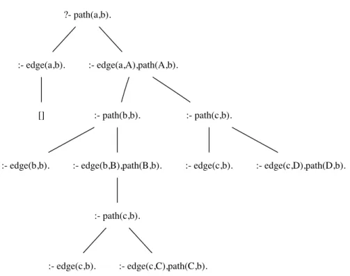
This process, which continues until the empty goal is reached, can be depicted by means of anSLD-tree. The root of such a tree corresponds to the query, each branch to aderivation, that is, a sequence of resolution steps. Derivations ending in the empty clause are also calledproofs.

(34)

12 FOUNDATIONS

?- path(a,b).

:- edge(a,b). :- edge(a,A),path(A,b).

[] :- path(b,b). :- path(c,b).

:- edge(b,b). :- edge(b,B),path(B,b). :- edge(c,b). :- edge(c,D),path(D,b).

:- path(c,b).

:- edge(c,b). :- edge(c,C),path(C,b).

Figure 2.1: SLD-tree for querypath(a,b) in Example 2.4.

Example 2.4 The following program encodes a graph with three nodes and defines paths between nodes in terms of edges.

edge(a,b). edge(a,c). edge(b,c).

path(X,Y) :− edge(X,Y).

path(X,Y) :− edge(X,Z),path(Z,Y).

Figure 2.1 shows the SLD-tree for query path(a,b), where the empty clause is

depicted by[].

By default, Prolog uses depth-first search to traverse the SLD-tree during proving, meaning that it can get trapped in infinite loops; however, this can be avoided by using alternative search strategies such as iterative deepening. Backtracking

forces the proving mechanism to undo previous steps to find alternative solutions. For example,nat(X)first returns answer substitution{X/0}as said above, but on

(35)

LOGIC PROGRAMMING 13

Normal logic programs use the notion ofnegation as failure, that is, for a ground atoma, not(a) is true exactly if acannot be proven in the program. They are

not guaranteed to have a unique minimal Herbrand model. Various ways to define the canonical model of such programs have been studied; here, we follow the

well-founded semanticsof Van Gelder et al. [1991]. It uses three-valued logic and partial models, that is, if the truth value of a literal is not determined by the program, it is considered undefined. Similarly to the least Herbrand model of definite clause programs, the well-founded model can be constructed iteratively by considering all clauses whose body is true in the current partial interpretation. However, during this construction, certain literals are also inferred to be false. The underlying idea is to set a set of literals to false if this makes it impossible to derive the value true for any of them. This is formalized using the concept of unfounded sets.

Given a normal logic program P with Herbrand base hb and a partial

interpretation I, a subset A ⊆ hb is unfounded if for each atom a ∈ A and

each grounded rulea:−b1, . . . , bn inP, some positive or negative body literalbiis

false inIor some positive body literalbioccurs inA. In the first case, the rule body

is false in the current partial interpretation and thus also in all interpretations that could be obtained by specifying truth values for additional literals, meaning that the clause cannot be used to derivea. In the second case, using the clause to derive awould require the positive literalbi to be true. However, if we simultaneously set

all literals inAto false, the bodies of all such clauses are false and they could thus

not be used to derive any literal inAas true.

The iterative construction of the well-founded model extends the current interpretation Ik into Ik+1 using two steps. First, for each ground rule whose

body is true inIk, the head is set true inIk+1. Second, all atoms in the greatest

unfounded set with respect toIk are set false inIk+1. These steps are repeated

until the least fixed point is reached.

The well-founded model has been shown to be two-valued for several restricted classes of normal logic programs, including stratified and locally stratified programs. A programP is stratified if and only if each of its predicatespcan be assigned a

rankj such that it only depends positively on predicates of rank at mostj and

negatively on predicates of rank at mostj−1. It islocally stratified if all atoms

ain its Herbrand base can be assigned a rank j such that for any grounded rule a:−b1, . . . , bm, the rank of positive literalsbiis at mostj, that of negative ones

at mostj−1.

Prolog usesSLDNF-resolution, a combination of SLD-resolution with negation as finite failure, for inference in normal logic programs. Negated atoms are commonly required not toflounder, that is, their variables need to be bound on calling.

(36)

14 FOUNDATIONS

2.2 Distribution Semantics

The distribution semantics as rigorously defined by Sato [1995] provides a formal basis for extending logic programming with probabilistic elements. It is a generalization of the least Herbrand model semantics, where the main difference is that logic programs contain a set of dedicated facts whose truth values are not directly set totrueas in the least Herbrand model of a usual logic program, but

determined probabilistically. Once these truth values are fixed, the program again has a unique least model extending the partial interpretation, which of course can be different depending on the initially chosen assignments. The distribution semantics now defines a distribution over these least Herbrand models of the program by extending a joint probability distribution over the set of dedicated facts. In its basic form, where the joint distribution is defined using a set of independent random events, it is a well-known semantics for probabilistic logics that has been (re)defined multiple times in the literature, often under other names or in a more limited database setting; cf. for instance [Dantsin, 1991; Poole, 1993b; Fuhr, 2000; Poole, 2000; Dalvi and Suciu, 2004]. Sato has, however, formalized a more general setting, including the case of a countably infinite set of random variables and using arbitrary discrete distributions over these basic random variables, in his well-known distribution semantics. We briefly repeat the basic ideas in the following; for more details, the interested reader is referred to [Sato, 1995].

We assume a first order language with denumerably many predicate, constant and functor symbols. LetDB=F∪Rbe a definite clause program, whereF is a set

of unit clauses, calledfacts, andR is a set of (possibly non-unit) clauses, called rules. For simplicity, it is assumed thatDB is ground and denumerably infinite,

and no fact inF unifies with the head of a rule inR. The distribution semantics

can be viewed as a possible worlds semantics, where ground atoms are treated as random variables, and worlds thus correspond to interpretations assigning truth values to all ground atoms inDB.

The key idea of the distribution semantics is to extend abasic distribution PF over

subsets or interpretationsF0⊆F into a distributionPDB over the least Herbrand

models ofDB, exploiting the uniqueness of the least Herbrand model ofF0∪Rfor

each suchF0. We first illustrate this for the finite case by means of an example. Example 2.5 Given the definite clause programDB=F∪R with

F ={a(0), a(1)}

R={(b(0) :−a(0)),(b(1) :−a(1), b(0))}

we enumerate ground atoms inF andDBasha(0), a(1)iandha(0), b(0), a(1), b(1)i,

respectively. This allows us to denote interpretations as binary vectors, where the i-th bit denotes the truth value of the i-th atom in the corresponding enumeration.

(37)

DISTRIBUTION SEMANTICS 15

Based on this notation, we define the basic distribution PF overΩF ={0,1}2 as

PF(00) = 0.21 PF(01)= 0.04 PF(10) = 0.58 PF(11)= 0.17

PF is now extended to a distribution PDB overΩDB={0,1}4 by setting

PDB(ˆω) =PF(ω)

ifωˆ corresponds to the least Herbrand model of DB extendingω, andPDB(ˆω) = 0

otherwise, that is

PDB(0000) = 0.21 PDB(0010)= 0.04

PDB(1100) = 0.58 PDB(1111)= 0.17

For an arbitrary sentence G using the vocabulary of DB we define the set of

possible worlds ˆω∈ΩDB whereGis true as

[G] ={ωˆ∈ΩDB |ωˆ |=G}.

Given a distributionPDBover ΩDB, the probability ofGis defined as the probability

of the set [G], which in the finite case is PDB([G]) =

X

ˆ

ω∈[G]

PDB(ˆω) (2.1)

Example 2.6 Continuing our example, the probability of b(0)is PDB([b(0)]) =PDB({1100,1111}) = 0.58 + 0.17 = 0.75,

while that of∀x.b(x)is

PDB([∀x.b(x)]) =PDB([b(0)∧b(1)]) =PDB({1111}) = 0.17.

While for finitely many basic facts,PF and thusPDB can be defined by exhaustive

enumeration of ΩF, this is no longer possible for infiniteF. Sato showed how to

definePDB based on a series of finite distributionsP

(n)

F over interpretationsωn

of the firstn variables inF. For this to be possible, these distributions have to

satisfy thecompatibility condition, that is

P_F(n)(ωn) =P

(n+1)

F (ωn1) +P

(n+1)

F (ωn0) (2.2)

Intuitively, this condition ensures that if a sentenceGsatisfies thefinite support condition, that is, there are finitely many minimal subsets F0 ⊆ F such that F0 ∪R |= G, we can fix a suitable enumeration of F and restrict probability

calculations to a finite prefix of this enumeration covering all facts appearing in these minimal subsets. We do not go into further technical detail here, but instead illustrate one basic and popular choice of such distributionsP_F(n)by means of an

(38)

16 FOUNDATIONS

Example 2.7 We extend our example switching to successor notation for natural numbers.

F ={a(0), a(s(0)), a(s(s(0))), a(s(s(s(0)))), . . .}

R={(b(0) :−a(0)),(b(s(N)) :−a(s(N)), b(N))}

The basic sample space is nowΩF ={0,1}∞, that is, the space of countably infinite

Boolean vectors. We fix enumerations for ground atoms inF andDB extending the ones used above, that is, following the order of arguments and iterating between aand bin the case of DB. Again, an interpretation ofF, for exampleω= 110∞, leads to a unique model ofDB, in this caseωˆ= 11110∞.

We consider all random variables corresponding to ground facts inF to be mutually independent, and assign a probability of being true to each of them. For the sake of simplicity, we use the same probabilitypfor each fact. Consider now a finite prefixωn of an interpretation ω∈ΩF, wherem variables are assigned1. Given

the independence assumption, the joint probability of the firstn random variables taking valueωn is thus

P_F(n)(ωn) =pm·(1−p)n−m.

Clearly, this series of distributions respects the compatibility condition of Equation (2.2). To calculate the probability of b(s(s(0)) in our example, it is sufficient to useP_F(3), as the first three elements ofF already determine the truth value of the query, that is

PDB([b(s(s(0))]) =PDB({ωˆ ∈ΩDB|ωˆ6= 111111}) =P (3)

F (111) =p

3

Finally, let us remark that the key to the distribution semantics is the existence of a unique canonical model of the entire program given an interpretation of the basic facts. While in the original distribution semantics, R is a definite clause

program and thus has a unique least Herbrand model, it is equally possible to use the well-founded semantics as discussed in Section 2.1, but parameterized by the set of basic facts, and restrict the set of rulesRin such a way that for each two-valued

interpretation of the basic facts, the well-founded model ofDB is two-valued as

well. In this view,Ris closely related to the definitions in FO(ID) [Denecker and

Vennekens, 2007; Vennekens et al., 2009], but restricts rule bodies to conjunctions of literals instead of arbitrary first order formulae.

2.3 Probabilistic Logic Learning

The core concept of statistical relational learning (SRL) or probabilistic logic learning (PLL) is the combination of machine learning, statistical techniques and

(39)

PROBABILISTIC LOGIC LEARNING 17

reasoning in first order logic. Many variants of this theme have been studied, differing both in their logical and in their probabilistic language. Here, we will distinguish two main streams by means of the basic probabilistic framework they employ. We start with the framework we will use throughout this thesis, namely the addition ofindependent probabilistic alternativesto relational languages, and afterwards discuss relational extensions of graphical models, which encode dependencies between random variables by means of their underlying graphical structure.

2.3.1 Using Independent Probabilistic Alternatives

Aprobabilistic alternative2 _{is a basic random event with a finite number of different}

outcomes, such as tossing a coin or rolling a die. Sets of mutually independent probabilistic alternatives are commonly used to define joint distributions over such events. A simple probabilistic model following this idea areprobabilistic context free grammars (PCFGs) [Manning and Sch¨utze, 1999]. Formally, a PCFG is a tuple (Σ, N, S, R) where Σ, thealphabetof the language defined by the grammar,

is a finite set of symbols called terminal symbols, N is a finite set of so-called nonterminal symbols,S∈N is the designatedstart symbol,R a set of rules of the

formP :A→β withleft hand side A∈N andright hand sideβ ∈(Σ∪N)∗, that

is, a finite sequence of symbols from Σ∪N, wheredenotes the empty sequence,

andP ∈[0,1] such that the sum over all rules inRwith the same left hand sideA

is 1. As common for such grammars, we denote terminal and non-terminal symbols by lower and upper case letters, respectively, and simply write a PCFG as the set of rulesR with start symbolS, leaving Σ andN implicit. Sentences are derived

starting from S by replacing the leftmost nonterminal symbol Ain the current

intermediate sentence by someβ withP :A→β∈R, until no more replacements

are possible, where replacement bycorresponds to simply deletingA. The choice

of rule for givenAis governed by the probability distribution overA’s rules given

by their labelsP, and is independent of everything else, including replacements of

further occurrences ofA. Thus, the independent probabilistic alternatives of PCFGs

are the choices of rules during derivations, and the probability of a derivation is given as the product of the probability of all its rule applications. Furthermore, the probability of a sentenceω∈(Σ∪N)∗ is the sum of probabilities of all derivations

ending inω.

(40)

18 FOUNDATIONS

Example 2.8 The following grammar defines a probability distribution over all finite non-empty strings over the alphabet{a, b}.

0.3 :S→aX 0.5 :X→aX 0.6 :Y →aX

0.7 :S→bY 0.1 :X→bY 0.2 :Y →bY (2.3)

0.4 :X→ 0.2 :Y →

Note that the grammar does not contain ambiguities, that is, each sentence can be obtained by a single derivation only. For instance, the sentenceaab is generated by the derivation

S−→0.3 aX −→0.5 aaX −→0.1 aabY −→0.2 aab and thus has probability

0.3·0.5·0.1·0.2 = 0.003.

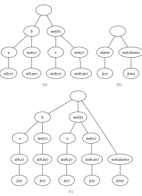
Stochastic Logic Programs (SLPs) [Muggleton, 1995] directly upgrade the idea of PCFGs to definite clauses, that is, instead of probability distributions over all rules with the same left hand side, they use probability distributions over all definite clauses with the same head predicate. Further probabilistic logic languages using independent probabilistic alternatives include the probabilistic logic programs of Dantsin [1991], PHA and ICL [Poole, 1993b, 2000], probabilistic Datalog [Fuhr, 2000], PRISM [Sato and Kameya, 2001], LPADs and CP-logic [Vennekens et al., 2004; Vennekens, 2007] and ProbLog as presented in Chapter 3 of this thesis; we will discuss this group of languages in more detail in Section 3.4. While most other formalisms use rule-based logical languages, FOProbLog [Bruynooghe et al., 2010] combines arbitrary first order formulae with independent probabilistic alternatives.

2.3.2 Using Graphical Models

While the probabilistic languages discussed in the previous section define joint distributions in terms of mutually independent random variables, in Bayesian Networks (BNs) [Pearl, 1988], a joint probability distribution over a finite set of random variables with finite domains is defined in terms of a conditional distribution for each variable given a subset of the others. More specifically, a BN is a directed acyclic graph whose nodes correspond to the random variables and whose edges represent direct dependencies between random variables. Each node in the network has an associated probability distribution over its values given the values of its

parents, the starting nodes of the node’s incoming edges. The full joint distribution over all variables is then given by the product of the individual distributions.

(41)

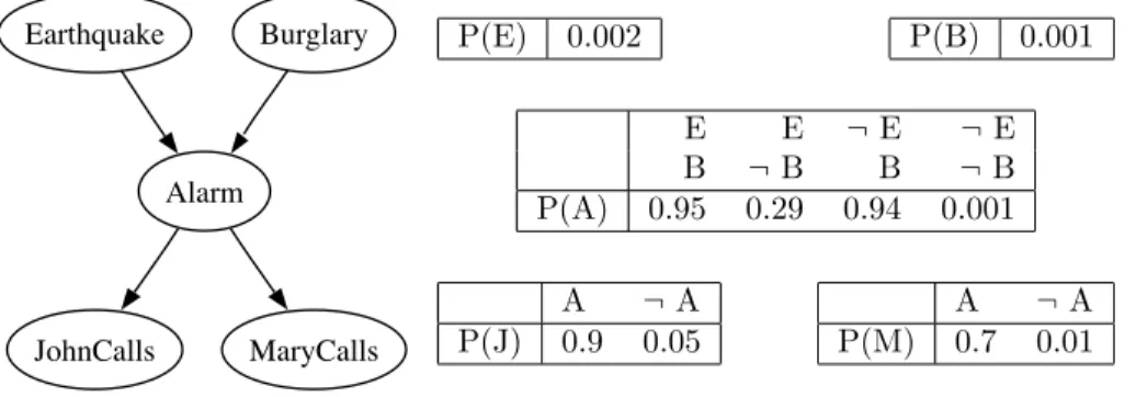
PROBABILISTIC LOGIC LEARNING 19 Earthquake Alarm JohnCalls MaryCalls Burglary _{P(E) 0.002} _{P(B) 0.001} E E ¬E ¬E B ¬B B ¬B P(A) 0.95 0.29 0.94 0.001 A ¬A P(J) 0.9 0.05 A ¬A P(M) 0.7 0.01 Figure 2.2: Bayesian network

Example 2.9 Figure 2.2 shows the well-known alarm Bayesian network [Pearl, 1988; Russell and Norvig, 2004], where all random variables have domain{0,1}.

It defines the joint distribution

P(E, B, A, J, M) =P(E)·P(B)·P(A|E, B)·P(J|A)·P(M|A) (2.4) For instance, the probability of{E= 1, B= 0, A= 1, J = 1, M = 1} thus is

P(1,0,1,1,1) = 0.002·(1−0.001)·0.29·0.9·0.7 = 0.000365

While Bayesian networks can be mirrored in terms of independent alternatives, as we will see in Section 3.4.1, inference for special purpose languages can directly exploit the underlying independencies.

Relational extensions of Bayesian networks typically specify the graph structure at an abstract level in some relational language and use this specification as a kind of template, from which concrete instances of Bayesian networks can be obtained by grounding out logical variables. Prominent examples of such extensions include Relational Bayesian Networks [J¨ager, 1997], Probabilistic Relational Models [Friedman et al., 1999], CLP(BN) [Santos Costa et al., 2003], Logical

Bayesian Networks [Fierens et al., 2005], Bayesian Logic Programs [Kersting and De Raedt, 2008], and P-log [Baral et al., 2009]. In contrast to these languages, Markov Logic Networks [Richardson and Domingos, 2006] are a first order variant of undirected graphical models, using weighted first order logic formulae as templates to construct Markov Networks, thereby defining probability distributions over possible worlds.

(42)

20 FOUNDATIONS x y y z z z z 0 0 0 1 1 1 1 1 (a) x y 1 z 0 (b)

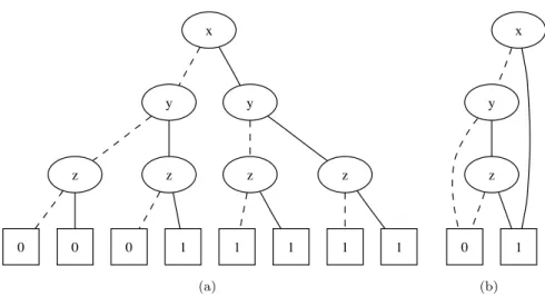
Figure 2.3: Full binary decision tree and corresponding BDD for formulax∨(y∧z);

dotted edges correspond to value 0, solid ones to 1.

2.4 Binary Decision Diagrams

A binary decision diagram (BDD) [Bryant, 1986] is a data structure that graphically represents a Boolean function. Roughly speaking, a BDD is a rooted directed acyclic graph, where nodes correspond to Boolean variables, edges to truth value assignments to their source node’s variable, and the two designated sink nodes, called 0- and 1-terminal node (or 0- and 1-leaf), to the function values 1 (or

true) and 0 (or f alse), respectively. Each path through such a diagram thus

encodes a truth value assignment together with the corresponding function value. While various variants of such diagrams exist, in this thesis, we will use the term BDD to refer toreduced ordered binary decision diagrams. As the name states, in this variant, all paths through the diagram respect the same variableordering, and furthermore, the diagram isreduced as much as possible to achieve maximal compression. We will now discuss the basics of BDDs by means of an example. Example 2.10 Consider the propositional formulax∨(y∧z), defining a Boolean function over three variables. Alternatively, this function could be specified by means of a truth table, that is, by listing all truth assignments to the variables together with the truth value of the formula. In Figure 2.3(a), such an explicit encoding is graphically depicted as a Boolean decision tree, where each branch corresponds to one assignment. Leaves are labeled with the truth value of the formula under the branch’s assignment. All edges are implicitly directed top-down. Dotted edges denote the assignment of 0 to the variable of their source node, solid ones that of1. Corresponding child nodes are called lowand highchild, respectively. The

(43)

BINARY DECISION DIAGRAMS 21

leftmost branch thus assigns0to all three variables, the next one assigns 0to both xandy, but1toz, and so forth. Clearly, already for such a small example, this encoding contains redundant information. For instance, once xis set to 1, the truth value of the entire formula is determined and the remaining tests listed in the corresponding subtree are unnecessary. The key idea of BDDs is to remove such redundancies by dropping nodes or sharing identical subtrees, which will transform the tree into a directed acyclic graph. For our example, this graph – which is a canonical representation given the variable ordering – is shown in Figure 2.3(b).

Two BDDsg1 andg2 areisomorphicif there exists a one-to-one mapping σfrom

edges ing1 to edges in g2 such that if σ(s1, t1) = (s2, t2), the edges (s1, t1) and

(s2, t2) are of the same type and each of the associated node pairs (s1, s2) and

(t1, t2) shares the same label. Starting from a full binary tree with the same variable

ordering on all branches, a BDD can be obtained using the following tworeduction operators:

Subgraph Merging If two subgraphs g1andg2are isomorphic, all edges leading

from some node outside g2 to some node in g2 are redirected to the

corresponding node ing1, and g2is removed from the graph.

Node Deletion If both outgoing edges of a nodenlead to the same node c, all

incoming edges ofnare redirected to c andnis removed from the graph. Example 2.11 In Figure 2.3(a), the two rightmost trees with root label z are isomorphic and can thus be merged, resulting in both outgoing edges of their parent nodey leading to the same node. Thus, this parent node can be deleted.

BDDs are one of the most popular data structures used within many branches of computer science, such as computer architecture and verification, even though their use is perhaps not yet so widespread in artificial intelligence and machine learning (but see [Chavira and Darwiche, 2007] and [Minato et al., 2007] for recent work on Bayesian networks using variants of BDDs). ProbLog is the first probabilistic logic programming system using BDDs as a basic data structure for probability calculation, a principle that receives increased interest in the fields of probabilistic logic learning and probabilistic databases, cf. for instance [Riguzzi, 2007; Ishihata et al., 2008; Olteanu and Huang, 2008; Thon et al., 2008; Riguzzi, 2009]. Since their introduction by Bryant [1986], there has been a lot of research on BDDs and their computation, leading to many variants of BDDs and off the shelf systems. The reduction approach to BDD construction described above is clearly impractical, as it starts from an exponential encoding of the Boolean formula. However, BDDs can also be constructed by applying Boolean operators to smaller BDDs, starting with BDDs corresponding to single variables and following the structure of the

(44)

22 FOUNDATIONS a b c 1 d e f 0 (a) a c c e e e e f 0 d d b b b b 1 (b)

Figure 2.4: Example illustrating the effect of variable ordering on BDD size for formula (a∧b)∨(c∧d)∨(e∧f), taken from [Bryant, 1986].

formula to be encoded, where reduction operators are applied on intermediate results. Denoting the number of nodes in a BDD g as |g|, reducing g has

time complexityO(|g| ·log(|g|)), while combiningg1andg2 has time complexity

O(|g1| · |g2|); for further details, we refer to [Bryant, 1986]. BDD tools construct

BDDs following a user-defined sequence of operations. The size of a BDD is highly dependent on its variable ordering, as this determines the amount of structure sharing that can be exploited for reduction; see Figure 2.4 for an example. As computing the order that minimizes the size of a BDD is a coNP-complete problem [Bryant, 1986], BDD packages include heuristics to reduce the size by reordering variables. While reordering is often necessary to handle large BDDs, it can be quite expensive. To control the complexity of BDD construction, it is therefore crucial to aim at small intermediate BDDs and to avoid redundant steps when specifying the sequence of operations to be performed by the BDD tool.