Verifying Procedural Programs via Constrained Rewriting Induction
CARSTEN FUHS, Birkbeck, University of London
CYNTHIA KOP, University of Innsbruck and University of Copenhagen NAOKI NISHIDA, Nagoya University
This paper aims to develop a verification method for procedural programs via a transformation into Logically Constrained Term Rewriting Systems (LCTRSs). To this end, we extend transformation methods based on integer TRSs to handle arbitrary data types, global variables, function calls and arrays, as well as encode safety checks. Then we adapt existing rewriting induction methods to LCTRSs and propose a simple yet effective method to generalize equations. We show that we can automatically verify memory safety and prove correctness of realistic functions. Our approach proves equivalence between two implementations, so in contrast to other works, we do not require an explicit specification in a separate specification language. Categories and Subject Descriptors: D.2.4 [Software Engineering]: Software/Program Verification; I.2.3 [Artificial Intelligence]: Deduction and Theorem Proving
General Terms: Formal Verification
Additional Key Words and Phrases: constrained term rewriting, inductive theorem proving, rewriting in-duction, lemma generation, program analysis
ACM Reference Format:
Carsten Fuhs, Cynthia Kop, and Naoki Nishida, 2017. Verifying Procedural Programs via Constrained Rewriting Induction.ACM Trans. Comput. LogicV, N, Article A ( YYYY), 46 pages.
DOI:http://dx.doi.org/10.1145/0000000.0000000
1. INTRODUCTION
Ensuring with certainty that a program always behaves correctly is a hard problem. One approach to this is formal verification—proving with mathematical rigor that all executions of the program will have the expected outcome. Several methods for this have been investigated (see e.g., [Huth and Ryan 2000]). However, classically many of them require expert knowledge to manually prove relevant properties about the code. Instead, we hope to raise the degree of automation, ideally creating a fully automatic verification / refutation process and tools to raise developer productivity. Indeed, over the last years automatic provers for program verification have flourished, as witnessed, e.g., by tool competitions like SV-COMP [SV-COMP] and the Termination Competition (http://termination-portal.org/wiki/Termination Competition). Program verification is also recognized in industry, cf. e.g. Facebook’s safety proverInfer[Calcagno et al. 2015] or Microsoft’s temporal prover T2 [Brockschmidt et al. 2016]. However, these tools generally use specific reasoning techniques for imperative programs and benefit from This work is supported by Austrian Science Fund (FWF) international project I963, Marie Skłodowska-Curie action “HORIP” (H2020-MSCA-IF-2014, 658162), the Japan Society for the Promotion of Science (JSPS), and Nagoya University’s Graduate Program for Real-World Data Circulation Leaders fromMEXT, Japan. Authors’ addresses: C. Fuhs, Dept. of Comp. Sci. and Inf. Sys., Birkbeck, Univ. of London, UK; C. Kop, Dept. of Comp. Sci., Univ. of Copenhagen, Denmark; N. Nishida, Grad. School of Informatics, Nagoya Univ., Japan. Permission to make digital or hard copies of part or all of this work for personal or classroom use is granted without fee provided that copies are not made or distributed for profit or commercial advantage and that copies show this notice on the first page or initial screen of a display along with the full citation. Copyrights for components of this work owned by others than ACM must be honored. Abstracting with credit is per-mitted. To copy otherwise, to republish, to post on servers, to redistribute to lists, or to use any component of this work in other works requires prior specific permission and/or a fee. Permissions may be requested from Publications Dept., ACM, Inc., 2 Penn Plaza, Suite 701, New York, NY 10121-0701 USA, fax+1 (212) 869-0481, or [email protected].
c
YYYY ACM 1529-3785/YYYY/-ARTA $15.00
the progress in automated theorem proving over the last decades only to a limited extent. This suggests likely avenues for improvement.
One such avenue isinductive theorem proving. This method is well investigated in functional programming [Bundy 2001] and term rewriting, the underlying core calcu-lus of functional programming. To check a functional programf against a specification by a reference implementationfspec, it suffices thatf(−→x) ≈ fspec(−→x) is an inductive
theorem. Thus, no explicit specification language is needed: giving a (possibly not opti-mized) reference implementationfspecin the same programming language suffices.
To analyze imperative programs (in C, Java, etc.), recent works have applied trans-formations into term rewrite systems (e.g., [Otto et al. 2010]). In particular, con-strained rewriting systemsare popular as target language, since logical constraints to model the control flow can be separated from terms to model intermediate states [Fu-ruichi et al. 2008; Falke and Kapur 2009; Sakata et al. 2009; Nakabayashi et al. 2010; Falke et al. 2011]. Unifying existing approaches, Kop and Nishida [2013] have pro-posed the framework oflogically constrained term rewriting systems (LCTRSs). Aims.The aim of this paper is twofold. First, we propose a new transformation method from procedural programs into constrained term rewriting. This transformation makes it possible to use the many methods available to term rewriting also to analyze imper-ative programs. Unlike previous methods, we do not limit interest to integer functions. Second, we develop a verification method for LCTRSs, based on rewriting induc-tion [Reddy 1990]—a well-investigated method of inductive theorem proving—to prove (total) equivalence of two functions. We also supply two generalization techniques, the main one of which is specialized for transformed iterative functions.
The applications are many. First, checking equivalence between different implemen-tations comes to mind. This allows the user to determine automatically if a modifica-tion in the program has changed its semantics (see e.g. [Godlin and Strichman 2013; Lahiri et al. 2012]). Proposing equivalent replacements may even be done automati-cally, via algorithm recognition (see e.g. [Alias and Barthou 2003]).
In compilation, automated equivalence checking can validate correctness of compiler optimizations on a per-instance basis [Necula 2000; Pnueli et al. 1998] or once-and-for-all for a given optimization template [Kundu et al. 2009; Lopes and Monteiro 2016]. Equivalence checking is also used in proofs of secure information flow [Terauchi and Aiken 2005] and can be used to prove safety properties, e.g., memory safety.
Why LCTRSs.Direct support of basic types like the integers, and of constraints to re-strict evaluation—features absent in basic TRSs—is essential to handle realistic pro-grams. Unlike earlier constrained rewriting systems, LCTRSs do not limit the under-lying theory to (linear) integer arithmetic: we might use (combinations of) arbitrary first-order theories, including, e.g.,n-dimensional integer arrays, floating point num-bers, and bitvectors. This makes it possible to natively handle sophisticated programs. Despite the generality, we get strong results on LCTRSs by reducing analysis prob-lems like termination and equivalence to a sequence of satisfiability probprob-lems over the underlying theories. Automatic tools—like our toolCtrl[Kop and Nishida 2015] for rewriting, termination, and inductive theorem proving—can defer such queries to an externalSAT Modulo Theories (SMT)solver [Nieuwenhuis et al. 2006], as a black box. Future advances in the SMT world then directly transfer to analysis of LCTRSs. Structure.We first recall the LCTRS formalism from [Kop and Nishida 2013] (§2) and show a way to translate procedural programs to LCTRSs (§3). Then we lift rewriting induction methods for constrained rewriting to LCTRSs (§ 4) and strengthen them with two dedicated generalization techniques (§5). Finally we discuss automation and experimental results (§6) as well as related and future work (§§7–8) and conclude.
Contributions over the conference version. The present paper provides several addi-tional contributions over the conference version [Kop and Nishida 2014]: (1) We signif-icantly extend our method to translate procedural programs to LCTRSs. (2) We extend our theory of constrained inductive theorem proving todisprovingequivalence (follow-ing [Sakata et al. 2009; Falke and Kapur 2012]) and add several inference rules. (3) We provide an additional generalization technique and a detailed proof strategy to au-tomate rewriting induction for translated procedural programs. (4) We have improved the implementation and added an automatic translation from C programs to LCTRSs. 1.1. Motivating Example
Aside from business applications, automatic equivalence proving can be used as an aid in grading student programming assignments. Combining a test run of the assign-ments on a set of sample inputs (which identifies many incorrect programs, but leaves false positives) with an automatic correctness check can save teachers a lot of time.
Example 1.1. Consider the following programming assignment.
Write a functionsum which, given an integer array and its length as input, returns the sum of its elements. Do not modify the input array.
We consider four different C implementations of this exercise:
int sum1(int arr[],int n){ int ret=0;
for(int i=0;i<n;i++) ret+=arr[i]; return ret; }
int sum2(int arr[], int n) { int ret, i; for (i = 0; i < n; i++) { ret += arr[i]; } return ret; }
int sum3(int arr[], int len) { int i;
for (i = 0; i < len-1; i++) arr[i+1] += arr[i]; return arr[len-1]; }
int sum4(int *arr, int k) { if (k <= 0) return 0; return arr[k-1] +
sum4(arr, k-1); }
The first solution is correct. The second is not, becauseretis not initialized—which may be missed in standard tests depending on the compiler used. The third solution is incorrect because the array is modified against the instructions, and moreover, gives a random result or segmentation fault iflen= 0. The fourth solution is correct.
These implementations can be transformed into the following LCTRSs: (1a) sum1(arr, n) → u(arr, n,0,0)
(1b) u(arr, n, ret, i) → error [i < n∧(i <0∨i≥size(arr))]
(1c) u(arr, n, ret, i) → u(arr, n, ret+select(arr, i), i+1) [i < n∧0≤i <size(arr)]
(1d) u(arr, n, ret, i) → return(arr, ret) [i≥n]
(2a) sum2(arr, n) → u(arr, n, ret,0) urules as copied from above (3a) sum3(arr, len) → v(arr, len,0)
(3b) v(arr, len, i) → error [i < len−1∧(i <0∨i+ 1≥size(arr))]
(3c) v(arr, len, i) → v(store(arr, i+ 1,select(arr, i+1) +select(arr, i)), len, i+1) [i < len−1∧0≤i∧i+ 1<size(arr)]
(3d) v(arr, len, i) → return(arr,select(arr, len−1))
[i≥len−1∧0≤len−1<size(arr)]
(3e) v(arr, len, i) → error [i≥len−1∧(len−1<0∨len−1≥size(arr))]
(4a) sum4(arr, k) → return(arr,0) [k≤0]
(4b) sum4(arr, k) → error [k−1≥size(arr)]
(4c) sum4(arr, k) → w(select(arr, k−1),sum4(arr, k−1)) [0≤k−1<size(arr)]
(4d) w(n,error) → error
(4e) w(n,return(a, r)) → return(a, n+r)
Note that arrays carry an implicit size (their allocated memory) which is queried to model the runtime behavior of the C program and test for out-of-bound errors. The fresh variable in the right-hand side of (2a)models that the third parameter ofu is assigned anarbitraryinteger. The details of this transformation are discussed in§3.
Using inductive theorem proving, we can now prove that
—∀arr∈array(int).∀len∈int. sum1(arr, len)↔∗sum4(arr, len)if0≤len≤size(arr)
—∃arr∈array(int).∃len∈int. sum3(arr, len)6↔∗sum4(arr, len)with0≤len≤size(arr)
So sum1 and sum4 return the same result on any input such that the given length does not cause out-of-bound errors, butsum3andsum4do not. (It seems likely that the disproof obtained from inductive theorem proving could be used to extract counterex-ample inputs, but at present we have not studied a systematic way of doing so.)
For sum2, wedohave sum2(arr, len) ↔∗ sum4(arr, len), since wecanalways choose
to instantiate retwith 0. The system is not confluent; we can also prove that there exista, nsuch thatsum2(a, n)→∗ s6=t←∗ sum4(a, n)for termss, tin normal form. As
explained in§6, we use a proof strategy which typically proves only the “6=” statement. 1.2. Practical Use
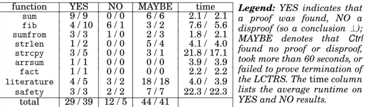
The primary application that we see for our technique is the following:
1.2.1. Comparing a function to a specification. As in Ex. 1.1, we can verify correctness of a C function f against a reference implementation g by translating both functions to LCTRS rules (§ 3) and proving that f(x1, . . . , xn) ≈ g(x1, . . . , xn) [true] is an
induc-tive theorem. If we only need equivalence under given preconditions on the input variables—such as 0 ≤ len ≤ size(arr)in Ex. 1.1—we formulate this as a constraint
ϕand analyze whetherf(x1, . . . , xn)≈g(x1, . . . , xn) [ϕ]is an inductive theorem.
Note that we do not require a separate specification language—although if desirable, it is of course possible to specify the reference implementation directly as an LCTRS.
Further possible applications of our technique include:
1.2.2. Code optimization (or other improvement).Sometimes the “reference implementa-tion” g suggested above can simply be an existing—and inefficient, or inelegant— version of a function. Thus, inductive theorem proving can be used to prove that it is safe to replace a function in a large real-life program by an optimized alternative.
1.2.3. Error checking.As the transformation from C to LCTRSs includes error checking (as seen for memory safety violations in Ex. 1.1), we can use inductive theorem proving to verify the absence of such errors. This is done by adding error-checking rules, e.g.,
errorfree(return(a, n)) → true errorfree(error) → false
and proving that errorfree(sum4(a, n)) ≈ true [ϕ] is an inductive theorem, where ϕ is the precondition on the input. Aside from memory safety, this approach can be used to certify the absence of for instance divisions by zero or integer overflow. The key is in the transformation, where we can choose which constructions result in an error.
1.2.4. Classical correctness checks.Aside from comparisons to an example implementa-tion, we can also specify a correctness property directly in SMT. For instance, given an implementation of thestrlenfunction, its correctness could be verified by proving that
strlen(x)≈return(n) [0≤n <size(x)∧select(x, n) =0∧ ∀i∈ {0, . . . , n−1}(select(x, i)6=0)]
is an inductive theorem. Alternatively, we can use extra rules to test properties in SMT. Example 1.2. To analyze correctness of an implementation ofstrcpy, we may use
test(x, n,error) → false
test(x, n,return(y)) → b[b⇔ ∀i∈ {0, . . . , n}(select(x, i) =select(y, i))]
and prove that the following equation is an inductive theorem:
test(x, n,strcpy(y, x))≈true
[0≤n <size(x)∧n <size(y)∧select(x, n) =0∧ ∀i∈ {0, . . . , n−1}(select(x, i)6=0)]
Note that this more sophisticated test isneededin this case, since correctness ofstrcpy
does not require thatx=yifstrcpy(x)→∗return(y)(the sizes ofxandymay differ).
2. PRELIMINARIES
In this section, we briefly recallLogically Constrained Term Rewriting Systems (usu-ally abbreviated asLCTRSs), following the definitions in [Kop and Nishida 2013]. 2.1. Logically Constrained Term Rewriting Systems
Many-sorted terms.We introduce terms, typing, substitutions, contexts, and subterms (with corresponding terminology) in the usual way for many-sorted term rewriting.
Definition 2.1. We assume given a set S ofsortsand an infinite setV of variables, each variable equipped with a sort. AsignatureΣis a set offunction symbolsf, disjoint fromV, each equipped with asort declaration[ι1× · · · ×ιn]⇒κ, with allιiandκsorts.
For readability, we often writeκinstead of[]⇒κ. The setTerms(Σ,V)oftermsoverΣ
andV contains any expressionssuch that`s:ιcan be derived for some sortι, using: `x:ι (x:ι∈ V)
`s1:ι1 . . . `sn :ιn
`f(s1, . . . , sn) :κ
(f : [ι1× · · · ×ιn]⇒κ∈Σ)
We fixΣandV. Note that for every terms, there is a unique sortιwith`s:ι. Definition 2.2. Let` s:ι. We callιthesort of s. LetVar(s)be the set of variables occurring ins; we say thatsisgroundifVar(s) =∅.
Definition 2.3. A substitution γ is a sort-preserving total mapping from V to Terms(Σ,V). The resultsγ of applying a substitutionγto a termsisswith all occur-rences of a variablexreplaced byγ(x). Thedomainofγ,Dom(γ), is the set of variables
xwith γ(x) 6= x. The notation[x1 := s1, . . . , xk := sk] denotes a substitution γ with
γ(xi) =si for1 ≤i≤n, andγ(y) =yfory /∈ {x1, . . . , xn}. For two substitutionsγand
δ, their compositionγ◦δis given by(γ◦δ)(x) =γ(δ(x)) = (xδ)γfor all variablesx. Two termssand t areunifiable if there exists a substitutionγ such thatsγ = tγ. Thenγis called aunifierforsandt. If moreover for all unifiersγ0forsandtthere is a substitutionδsuch thatγ0 =δ◦γ, we callγamost general unifier (mgu)forsandt.
Definition 2.4. Given a term s, apositionin sis a sequence pof positive integers such that s|p is defined, where s| = sandf(s1, . . . , sn)|i·p = (si)|p. We call s|p a
sub-term of s. If ` s|p : ι and ` t : ι, then s[t]p denotes s with the subterm at position
preplaced by t. Acontext C is a term containing one or more typedholes 2i : ιi. If
Logical terms.Specific to LCTRSs, we consider different kinds of symbols and terms. Definition 2.5. We assume given:
— signaturesΣterms andΣtheory such thatΣ = Σterms∪Σtheory;
— a mappingI which assigns to each sortιoccurring inΣtheory a setIι;
— a mappingJ which assigns to each f : [ι1 × · · · ×ιn] ⇒ κ ∈ Σtheory a function in Iι1× · · · × Iιn=⇒ Iκ;
— for all sorts ι occurring in Σtheory a set Valι ⊆ Σtheory of values: function symbols
a: []⇒ιsuch thatJ gives a bijective mapping fromValιtoIι.
We require that Σterms ∩Σtheory ⊆ Val = SιValι. The sorts occurring inΣtheory are calledtheory sorts, and the symbolstheory symbols. Symbols inΣtheory\ Valare
calcu-lation symbols. A term inTerms(Σtheory,V)is called alogical term.
Definition 2.6. For ground logical terms, letJf(s1, . . . , sn)K:=Jf(Js1K, . . . ,JsnK). For every ground logical termsthere is a unique valuecsuch thatJsK=JcK; we say thatcis the value ofs. Aconstraintis a logical termϕof some sortboolwithIbool=B={>,⊥}, the set ofbooleans. A constraintϕisvalidifJϕγK=>forallsubstitutionsγwhich map Var(ϕ)to values, andsatisfiableifJϕγK=>forsomesuch substitutions. A substitution
γrespectsϕifγ(x)is a value for allx∈Var(ϕ)andJϕγK=>.
Terms in Terms(Σterms,∅) can be thought of as the primary objects of rewriting: a reduction typically begins and ends with such terms, with elements of Σtheory \ Val (also calledcalculation symbols) to perform calculations in the underlying theory.
We typically choose a theory signature withΣtheory ⊇Σcoretheory, whereΣcoretheory contains
true,false:bool,∧,∨,⇒: [bool×bool]⇒bool,¬: [bool]⇒bool, and, for all theory sortsι, symbols=ι,6=ι: [ι×ι]⇒bool, and an evaluation functionJ that interprets these
sym-bols as expected. We omit the sort subscripts from=and6=when clear from context. Definition 2.7. The standard integer signatureΣint
theory isΣ core
theory ∪ {+,−,∗,exp,div,
mod: [int×int]⇒int;≤, <: [int×int]⇒bool} ∪ {n:int|n∈Z}with valuestrue, falseand nfor alln∈ Z. Thus, we usen(insans-seriffont) as the function symbol for n∈Z(in math font). We defineJ in the natural way, except: since allJf must be total functions,
we set Jdiv(n,0) = Jmod(n,0) = Jexp(n, k) = 0for allnand allk < 0. Of course, when constructing LCTRSs, we normally add explicit error checks to prevent such calls.
Example 2.8. LetS={int,bool}, andΣ = Σterms ∪Σinttheory, where
Σterms ={fact: [int]⇒int} ∪ {n:int|n∈Z}
Then bothintandboolare theory sorts. We also define set and function interpretations, i.e., Iint =Z,Ibool =B, andJ is defined as above. With=for=int and infix notation, examples of logical terms are0 = 0+−1 andx+3 ≥ y+−42. Both are constraints.
5+9is also a (ground) logical term, but not a constraint. Expected starting terms are, e.g.,fact(42)orfact(fact(−4)): ground terms fully built using symbols inΣterms.
Rules and rewriting.We adapt the standard notions of rewriting (see, e.g., [Baader and Nipkow 1998]) by including constraints and adding rules to perform calculations.
Definition 2.9. Aruleis a triple`→r[ϕ]with`andrterms of the same sort andϕa constraint. Here,`has the formf(`1, . . . , `n)and contains at least one symbol inΣterms\
Σtheory (so`is not a logical term). Ifϕ=truewithJ(true) =>, we may write`→r. We defineLVar(`→r[ϕ])asVar(ϕ)∪(Var(r)\Var(`)). A substitutionγrespects`→r[ϕ]
ifγ(x) ∈ Val for allx ∈ LVar(` → r[ϕ]), andJϕγK =>. The rule is left-linearif` is linear, i.e., all variables occur at most once in`, andirregularifVar(ϕ)\Var(`)6=∅.
Note that it is allowed to haveVar(r)6⊆Var(`), but fresh variables in the right-hand side may only be instantiated withvalues. This is done to model user input or random choice. Otherwise, variables outside the constraint may be instantiated by any term; we do not impose strategies like innermost or call-by-value reduction.
Definition 2.10. We assume given a set of rules R and let Rcalc be the set
{f(x1, . . . , xn) → y [y = f(−→x)] | f : [ι1× · · · ×ιn] ⇒ κ ∈ Σtheory \ Val} (writing −→x forx1, . . . , xn). Therewrite relation→Ris a binary relation on terms, defined by:
C[`γ] →R C[rγ] if`→r[ϕ]∈ R ∪ Rcalcandγrespects`→r[ϕ]
Here,Cis a context with exactly one hole. We say that the reduction occurs at position
pifC =C[2]p. Lets↔Rtifs→R tort →Rs. A reduction step withRcalc is called a
calculation. A term is innormal formif it cannot be reduced with →R. We say thatt
is anormal form ofsifs→∗
R tandtis a normal form. The relation→Risconfluentif
whenevers→∗
R tands→∗R t0, there exists also someuwitht→∗Ruandt0→∗Ru.
We usually call the elements ofRcalcrules—orcalculation rules–even though their
left-hand side is a logical term. Note that if→Ris confluent, every term has at most one
normal form (intuitively, thenRis deterministic with respect to big-step semantics). Definition 2.11. Forf(`1, . . . , `n)→r[ϕ]∈ Rwe callf adefined symbol; non-defined
elements ofΣterms and all values areconstructors. LetDbe the set of all defined sym-bols andConsthe set of constructors. A term inTerms(Cons,V)is aconstructor term.
Now we may define a logically constrained term rewriting system(LCTRS) as the abstract rewriting system(Terms(Σ,V),→R). An LCTRS is usually given by supplying
Σ,R, and an informal description ofIandJ if these are not clear from context. Example 2.12. To implement an LCTRS calculating thefactorialfunction, we use the signatureΣfrom Ex. 2.8 and the following rules:
Rfact={fact(x)→1[x≤0] , fact(x)→x∗fact(x−1) [¬(x≤0)]}
Using calculation steps, a term3−1reduces to2in one step (using the calculation rule
x−y → z [z =x−y]), and3∗(2∗(1∗1))reduces to6in three steps. Using also the rules inRfact,fact(3)reduces in ten steps to6.
Example 2.13. To implement an LCTRS calculating the sum of elements in an array, let Ibool = B, Iint = Z, Iarray(int) = Z∗, so array(int) is mapped to finite-length integer sequences. LetΣtheory = Σinttheory ∪ {size : [array(int)] ⇒ int, select : [array(int)×
int] ⇒ int} ∪ {a | a ∈ Z∗}. (We do notencode arrays as lists: every “array”—integer sequence—acorresponds to a unique symbola.) The interpretation functionJ behaves onΣint
theory as usual, maps the valuesato the corresponding integer sequence, and has: Jsize(a) = k ifa=hn0, . . . , nk−1i Jselect(a, i) = ni ifa=hn0, . . . , nk−1iand0≤i < k
0 otherwise
In addition, letΣterms ={sum,sum0: [array(int)]⇒int}∪{n:int|n∈Z}∪{a|a∈Z∗} and letRconsist of
sum(x) → sum0(x,size(x)−1) sum0(x, k) → select(x, k) +sum0(x, k−1) [k≥0]
sum0(x, k) → 0 [k <0]
Note that this implementation differs from the ones in Ex. 1.1, because there we an-alyzed encodings of imperative programs; on C level there is no functionality for the programmer to explicitly query the size of an array. Here, we avoided boundary checks.
Values are new in LCTRSs compared to older styles of constrained rewriting. These representatives of the underlying theory are always constants (constructor symbols which do not take arguments), even if they represent complex structures, as seen in Ex. 2.13. Note that variables in a rule’s constraintmustbe instantiated by values; for instance in Ex. 2.12, a termfact(1+2)must be reduced by a calculation first. We also do not match modulo theories, e.g., we do not equate0+ (x+y)withy+xfor matching. Differences to [Kop and Nishida 2013].In the original definition of LCTRSs, variables inV are unsorted, and a separate variable environmentis used for typing. Also,→R
is there defined as the union of two relations →rule and→calc rather than including
Rcalc. These changes give equivalent results, but the current definitions cause less bookkeeping. A larger difference is the restriction on rules: in [Kop and Nishida 2013] left-hand sides must have a root symbol inΣterms\Σtheory. We follow Kop [2013] and Kop and Nishida [2014] in weakening this (only asking that they are not logical terms). 2.2. Quantification
The definition of LCTRSs does not permit constraints with quantifiers (constraints are terms, and first-order rewriting does not allow quantifiers in terms). In, for instance, an LCTRS over integers and arrays, which hasaddtoend: [int×array(int)]⇒array(int)∈
Σtheory andextend: [array(int)×int]⇒array(int)∈Σterms, we cannot specify a rule like:
extend(arr, x)→addtoend(x,arr) [∀y∈ {0, . . . ,size(arr)−1}(x6=select(arr, y))]
However, one of the key features of LCTRSs is that theory symbols, including pred-icates, are not confined to a fixed list. Therefore, wecanadd a new symbol to Σtheory (andJ). For theextendrule, we might introduce a symbolnotin: [int×array(int)]⇒bool
with Jnotin(u,ha0, . . . , an−1i) = > iff for all i: u 6= ai, and replace the constraint by
notin(x,arr). This generates exactly the same reduction relation as the original rule. Thus, we can permit quantifiers in the constraints of rules and also on right-hand sides of rules, as an intuitive notation for fresh predicates. However, an unbounded quantification would likely not be useful, as it would give an undecidable relation→R.
Comment:One might argue that adding symbols like this is problematic in prac-tice: no SMT solver will support new symbols likenotin. However, for the tech-nique this makes no difference. In an implementation, we might allow quanti-fiers as syntactic sugar (and pass the same sugar to the SMT solver), or add a layer on top of the SMT solver which translates the new symbol(s), replacing for instance(notin u a)by(forall ((x Int)) (distinct u (select a x))). 2.3. Rewriting Constrained Terms
In LCTRSs, the objects of study are terms, with →R defining the relation between
them. However, for analysis it is often useful to considerconstrained terms:
Definition 2.14. A constrained term is a pairs[ϕ]of a termsand a constraintϕ. We says[ϕ]andt[ψ] areequivalent, notations[ϕ]∼ t[ψ], if for all substitutionsγ which respectϕthere is a substitutionδwhich respectsψsuch thatsγ=tδ, and vice versa.
Intuitively, a constrained terms[ϕ]represents all termssγwhereγrespectsϕ, and can be used to reason about such terms. Equivalent constrained terms represent the same set of terms; for examplef(0) [true]∼f(x) [x=0], andg(x, y) [x > y]∼g(z, u) [u≤
z−1]. Note thats[ϕ]∼s[ψ]if and only if∀−→x(∃−→y (ϕ)↔ ∃−→z (ψ))holds, whereVar(s) =
{−→x},Var(ϕ)\Var(s) ={−→y }andVar(ψ)\Var(s) ={−→z }.
Definition 2.15. For a ruleρ:=`→r[ψ]∈ R ∪ Rcalcand positionq, we lets[ϕ]→ρ,q
variable inVar(ϕ)for allx∈LVar(`→r[ψ]), andϕ⇒(ψγ)is valid. Lets[ϕ]→baset[ϕ]
if s[ϕ] →ρ,q t[ϕ] for some ρ, q. The relation →R on constrained terms is defined as
∼ · →base· ∼. We say thats[ϕ]→Rt[ψ]at positionqby ruleρifs[ϕ]∼ · →ρ,q· ∼t[ψ].
Example 2.16. In the LCTRS from Ex. 2.12, we havefact(x) [x >3]→Rx∗fact(x− 1) [x >3]. Now we can use a calculation rulex−y→z[z=x−y], with a non-empty ∼-step, as follows:x∗fact(x−1) [x >3]∼x∗fact(x−1) [x >3∧z=x−1]→basex∗fact(z) [x >
3∧z=x−1]. The∼-relation holds because indeed∀x(x >3↔ ∃z(x >3∧z=x−1)). Example 2.17. The∼-relation also allows us to reformulate the constraint after a reduction. For example, with the rule f(x) → g(y) [y > x], we have: f(x) [x > 3] ∼
f(x) [x > 3∧y > x] →base g(y) [x > 3∧y > x] ∼ g(y) [y > 4]. We do not have that
f(x) [true]→R g(x+1) [true], asx+1cannot be instantiated to a value.
Example 2.18. A constrained term does not always need to be reduced in the most general way. With the rulef(x)→g(y) [y > x], we havef(0) [true]∼f(0) [y >0]→base
g(y) [y >0], but we also havef(0) [true]∼f(0) [1>0]→baseg(1) [1>0]∼g(1) [true].
As intended, constrained reductions give information about usual reductions:
THEOREM 2.19. Ifs[ϕ]→R t[ψ], then for all substitutionsγwhich respectϕthere existsδwhich respectsψsuch thatsγ→Rtδ. Both steps use the same rule and position.
PROOF. We first observe (**): Ifu[ξ]→base q[ξ], then for any substitutionγ which
respectsξalsouγ →Rqγ. Proof: ifu[ξ]→baseq[ξ], then there arep, `→r[c]andδsuch
thatu|p =`δ,q=u[rδ]p,δ(x)∈Var(ξ)∪ Valfor allx∈LVar(`→r[c])andξ⇒(cδ)is
valid. Withη=γ◦δ, we have(uγ)|p =u|pγ=`δγ =`ηandqγ=u[rδ]pγ= (uγ)[rδγ]p=
(uγ)[rη]p. We also haveη(x) =δ(x)γ∈ Valforx∈LVar(`→r[c])becauseγrespectsξ
and, sinceJξγK=>andξ⇒(cδ)is valid, alsoJ(cδ)γK=JcηK=>. So indeeduγ →Rqγ.
Now, supposes[ϕ]→R t[ϕ], sos[ϕ]∼s0[ξ]→baset0[ξ]∼t[ψ], and letγrespectϕ. By
definition of∼, there is some substitutionηwhich respectsξsuch thatsγ=s0η. By (**)
s0η→R t0η. Again by definition of∼, we findδwhich respectsψsuch thatt0η =tδ.
THEOREM 2.20. Ifs[ϕ] →R t[ψ], then for all substitutionsδwhich respectψthere existsγwhich respectsϕsuch thatsγ→Rtδ. Both steps use the same rule and position.
PROOF. Parallel to the proof of Thm. 2.19: ifs[ϕ]∼s0[ξ]→base t0[ξ]∼t[ψ], then by
definition of∼there are suitableη, γsuch thattδ=t0η←Rs0η=sγ.
Comment:The relation →R on constrained terms isnot stable: for instance, in
the system from Ex. 2.18, we can derive f(x) [true] →R g(x) [true] even though f(0) [true]6→R g(0) [true]. This is because the variables in a constrained terms[ϕ]
are fully changeable; one can see variables inVar(s)as universal and the oth-ers as existential. This is not problematic, as we do not instantiate constrained terms; to reason with constrained reduction we only use Theorems 2.19 and 2.20. 3. TRANSFORMING IMPERATIVE PROGRAMS INTO LCTRSS
Equivalence-preserving transformations of imperative programs into constrained rewriting systems operating on integers have been investigated in e.g. [Falke and Ka-pur 2009; Falke et al. 2011; Furuichi et al. 2008]; more generally, such translations from imperative to functional programs have been investigated at least since [Mc-Carthy 1960]. Although these papers use different definitions of constrained rewrit-ing, the proposed transformations can be adapted to produce LCTRSs that operate on integers, i.e., useΣtheory as in Ex. 2.12. What is more, we can extend the ideas to also handle more advanced programming structures, such as arrays and exceptions.
In this section, we will discuss a number of ideas towards a translation from C to LCTRS. A more detailed and formal treatment of the limitation to integers and one-dimensional integer arrays is available online along with an implementation, at:
http://www.trs.css.i.nagoya-u.ac.jp/c2lctrs/
Given the extensiveness of the C specification, we will not attempt to prove that the result of our transformation corresponds to the origin. Instead, we shall rely on an appeal to intuition. An advantage is that the same ideas apply to other programming languages; we should be able to use similar translations for, e.g., Python or Java. 3.1. Transforming Simple Integer Functions
The base form of the transformation—limited to integer functions with no global vari-ables or function calls—is very similar to the transformations for integer TRSs in [Falke and Kapur 2009; Falke et al. 2011; Furuichi et al. 2008]. Each function is trans-formed separately. We introduce a function symbol for every statement (including dec-larations), which operates on the variables in scope. The transition from one statement to another is encoded as a rule, with assignments reflected by argument updates in the right-hand side, and conditions by the constraint. Return statements are encoded by reducing to an expressionreturnf(e), wherereturnf : [int]⇒resultf is a constructor.
Example 3.1. Consider the following C function and its translation:
int fact(int x) { int z = 1;
for (int i = 1; i <= x; i++) z *= i; return z; } fact(x) →u1(x,1) u1(x, z) →u2(x, z,1) u2(x, z, i) →u3(x, z, i) [i≤x] u2(x, z, i) →u5(x, z) [¬(i≤x)] u3(x, z, i) →u4(x, z∗i, i) u4(x, z, i) →u2(x, z, i+1) u5(x, z) →returnfact(z)
ForΣtheory we assume the standard integer signature;Σterms containsfact, allui and
the constructorreturnf, all of which have output sortresultf and argument sortsint.
A realistic translation of C code must also handle the absence of a boolean data type, operator precedence, and expressions with side effects (e.g., a loop condition--x). All this is easily doable1(and included in our implementation), but for the sake of brevity we will not go into detail here.
Finally, the generated system is optimized to make it more amenable to analysis:2 — rules are combined where possible, e.g., replacing a pair of rules`→u(r1, . . . , rn) [ϕ]
andu(x1, . . . , xn)→s[true]by`→s[x1:=r1, . . . , xn:=rn]ifuis not used elsewhere;
— unused arguments of function symbols are removed, such as the second (but not the first!) argument ofuin an LCTRS with rulesu(x, y, z)→u(x−1, y+1, z∗2) [x > 0]
andu(x, y, z)→return(z) [¬(x >0)];
— constraints are simplified, for instance replacing¬(x >0)byx≤0in the rules above. We will use these optimizations also for the extended transformations of§§3.2–3.6.
Comment:Whentime complexity—defined as, e.g., the number of certain calcula-tion steps—is considered, the argument removal step is dangerous, as it may re-move calculations. In such cases we would use a different simplification method.
1This is discussed in the formal treatment at http://www.trs.css.i.nagoya-u.ac.jp/c2lctrs/formal.pdf
2Variations of such preprocessing steps preserving the properties of interest to simplify the output of an
automatic translation are fairly standard in program analysis, see e.g. [Albert et al. 2008; Alpuente et al. 2007; Beyer et al. 2009; Falke et al. 2011; Giesl et al. 2017; Spoto et al. 2009].
Example 3.2. Optimizing the LCTRS from Ex. 3.1, we obtain:
fact(x) →u2(x,1,1) u2(x, z, i) →u2(x, z∗i, i+1) [i≤x] u2(x, z, i) →returnfact(z) [i > x]
Differences to older work. In contrast to existing transformations to integer TRSs (e.g. [Falke and Kapur 2009; Falke et al. 2011; Furuichi et al. 2008]), we do not consider basic blocks, but simply create rules for every statement; this gives no substantial dif-ference after optimization. Additionally,returnf is new here: in the work by Falke et al,
the return statement is omitted, as they focus ontermination, while in [Furuichi et al. 2008] the final term reduces directly to the return-value, e.g.u4(x, z)→z+x[x≤0].
3.2. Non-Integer Data Types
Integers are not special: as the definition of LCTRSs permits arbitrary theories, we can handle any data type in C. We might for instance interpretdoubleas either real num-bers or double-precision floating point numnum-bers; this choice is left to the user and may vary by application. The only requirement is that a suitable theory signature—with corresponding SMT solver if the system is to be analyzed automatically—is available. The translation is straightforward, with the only difficulty that type casts must be made explicit, and we need to use separate symbols such as+.fordoubleaddition.
Example 3.3. Consider the following C function and its translation.
double halfsum(double thold) { double ret = 0.0;
for (int d = 2; d < 100; d *= 2) { ret += 1.0 / d;
if (ret > thold) return ret; } } halfsum(t) → u2(t,0.0,2) u2(t, r, d) → u4(t, r+.1.0/todouble(d), d) [d <100] u2(t, r, d) → returnhalfsum(rnd) [d≥100] u4(t, r, d) → returnhalfsum(r) [r >. t] u4(t, r, d) → u2(t, r, d∗2) [r≤. t]
This demonstrates both an explicit cast and one possible way to handle an undefined return value (by a fresh variable, which may be instantiated with a random value). 3.3. Error Handling
The transformation of§3.1 does not fully reflect the original C program: as computers have limited memory, integers are internally represented asbitvectors. To address this, we could change the theory. Rather than usingZ, we letValint ={MININT, . . . ,MAXINT} and make J+,J−, and J∗ wrap around (e.g., J−(MININT,1) = MAXINT). The resulting
LCTRS has the same rules, but acts more closely to the real program behavior. However, integer overflow is often indicative of anerror. Indeed, in C an overflow for the typeintleads to undefined behavior (which also surfaces in optimizing compilers such asgccorclang). In order to model this (or other instances of undefined behavior in C, such as a missingreturnstatement), we will reduce to a specialerrorstate.
Thus, for every ruleui(x1, . . . , xn)→r[ϕ]: if this rule represents a transition where
an error may occur under conditionτ, then we split it in two:
ui(x1, . . . , xn)→r[ϕ∧ ¬τ] ui(x1, . . . , xn)→errorf [ϕ∧τ]
As usual, we simplify the resulting constraint (writing, e.g.,x <0instead of¬(x≥0)). Example 3.4. Continuing Ex. 3.2, we generate the following rewrite rules:
fact(x) →u2(x,1,1)
u2(x, z, i) →u2(x, z∗i, i+1) [i≤x∧z∗i≤MAXINT∧z∗i≥MININT∧i+1≤MAXINT] u2(x, z, i) →errorfact [i≤x∧(z∗i >MAXINT∨z∗i <MININT∨i+1>MAXINT)]
Note that we could easily model assertions andthrowstatements for exceptions in the same way. Division by zero is handled in a similar way.
We can choose whether to add error transitions before or after the simplification step. The distinction is important: when simplifying, calculations which do not contribute to the final result are thrown away. In the case of overflow errors, it may seem reasonable to consider the post-simplification rules, as we did in Ex. 3.4. In the case of for instance division by zero, we should add the errors to the pre-simplification rules.
Comment: When transforming a function into an LCTRS, we can choose what errors to model. For instance, we could ignore overflows (effectively assuming unbounded integers), but still test for division by zero. We could also leterrorf be
a constructor which takes an argument, i.e.,errorf : [Errors] ⇒ resultf ∈ Σterms, whereErrorsis a sort with constructorsIntegerOverflow,DivisionByZero, and so on. 3.4. Global Variables
Thus far, we have considered very localcode: a function never calls other functions or modifies global variables. By altering thereturnconstructors, we easily change the latter: we assume that a function symbol is given all global variables that it uses as input, and that it returns those global variables it alters as output, along with its return value. This change also allows for non-redundantvoidfunctions.
Example 3.5. Consider the following short program and its (simplified) translation:
int best; int up(int x) {
if (x > best) { best = x; return 1; } return 0;
}
up(b, x) → returnup(x,1) [x > b]
up(b, x) → returnup(b,0) [x≤b]
3.5. Function Calls
Next, let us consider function calls. A difficulty is that they may occur in an expres-sion, e.g.,fact(3) +5, which is not well sorted in the corresponding LCTRS:fact(3)has sortresultfact, notint. To avoid this issue, and to propagate errors, we split off function calls occurring inside expressions other thanvar =func(arg1, . . . ,argn)and store their return value into a temporary variable. For example:
int ncr(int x, int y) { int a = fact(x);
int b = fact(y) * fact(x - y); return a / b;
}
=
⇒
int ncr(int x, int y) { int a = fact(x); int tmp1 = fact(y); int tmp2 = fact(x - y); int b = tmp1 * tmp2; return a / b;
}
This change may cause declarations at places in the function where a C compiler would not accept them, but for the translation, this is no issue. We translate the result-ing function by executresult-ing function calls in a separate parameter and usresult-ing a separate step to examine the outcome of a function call and assign it to the relevant variable(s). Example 3.6. The ncr program above is transformed to the following optimized LCTRS (where we test for division by zero but not integer overflow for simplicity):
ncr(x, y) → u2(x, y,fact(x)) u2(x, y,errorfact) → errorncr
u2(x, y,returnfact(k)) → u3(x, y, k,fact(y)) u3(x, y, a,errorfact) → errorncr
u3(x, y, a,returnfact(k)) → u4(x, y, a, k,fact(x−y)) u4(x, y, a, t1,errorfact) → errorncr
u4(x, y, a, t1,returnfact(k)) → errorncr [t1∗k=0] u4(x, y, a, t1,returnfact(k)) → returnncr(adiv(t1∗k)) [t1∗k6=0]
3.6. Statically Allocated Arrays
Finally, let us consider arrays. After we have seen Ex. 1.1 and the way side effects were handled in§3.4, this is largely as expected. For now, we will not consider aliasing.
To start, we must fix a theory signature and corresponding interpretations. For a given theory sort ι which admits at least one value, say0ι, letarray(ι)be a new sort
and Iarray(ι) = Iι∗—so each value corresponds to a finite sequence. We introduce the
following theory symbols (in addition toΣinttheory and other desired theories): —sizeι : [array(ι)]⇒int: we defineJsizeι(a)as the length of the sequencea.
—selectι : [array(ι)×int]⇒ι: ifa=ha0, . . . , an−1i, we defineJselectι(a, k) =ak if0≤k < n andJselectι(a, k) =0ι otherwise.
—storeι : [array(ι)×int×ι] ⇒ array(ι): if a = ha0, . . . , an−1i, we define Jstoreι(a, k, v) = ha0, . . . , ak−1, v, ak+1, . . . , an−1iif0≤k < nandJstoreι(a, k, v) =aotherwise.
We will usually omit the subscriptιwhen the sort is clear from context.
Our arrays are different from SMT-LIB (cf. http://www.smt-lib.org/), where arrays are functions from one (possibly infinite) domain to another. For program analysis, finite-length sequences seem practical instead. SMT problems on our arrays can be translated to SMT-LIB format using an additional integer variableasizefor the size of an arrayaand universal quantification to set entries outside the array to a fixed value. We encodelookupsa[i]asselect(a, i); forassignmentsa[i] =e, we replaceabystore(a, i, e). To ensure correctness here, we add boundary checks to the constraint and reduce toerrorf if such a check is not satisfied. After an assignment, the updated variable is
included in the return value since the underlying memory of the array was altered. Example 3.7. Consider the following C implementation of the strcpy function, which copies the contents oforiginalinto the arraygoal, until a0is reached.
void strcpy(char goal[], char original[]) { int i = 0;
for (; original[i] != 0; i++) goal[i] = original[i]; goal[i] = 0;
}
For simplicity, we think of strings as integer arrays (although alternative choices forIcharmake little difference). The function never updatesoriginal, but may update
goal, so the return value must include the latter. We obtain the following LCTRS:
strcpy(gl, org) → v(gl, org,0)
v(gl, org, i) → errorstrcpy [i <0∨i≥size(org)]
v(gl, org, i) → w(gl, org, i) [0≤i <size(org)∧select(org, i) =0]
v(gl, org, i) → errorstrcpy [0≤i <size(org)∧select(org, i)6=0∧i≥size(gl)]
v(gl, org, i) → v(store(gl, i,select(org, i)), org, i+1)
[0≤i <size(org)∧select(org, i)6=0∧i <size(gl)] w(gl, org, i) → errorstrcpy [i <0∨i≥size(gl)]
w(gl, org, i) → returnstrcpy(store(gl, i,0)) [0≤i <size(gl)]
Here, the notation0≤i <size(org)is shorthand for0≤i∧i <size(org). Note that this LCTRS could be further simplified by combining the third rule with the last two rules.
Comment:It should now be clear how the systems from§1.1 have been translated from C code to LCTRSs. The only deviation is that there we have included the arrayarr in the return value ofsum1,sum2, andsum4, which is not necessary as it is not modified in these cases. This was done to allow for a direct comparison withsum3, where the arrayismodified. In addition, thereturnanderrorsymbols in these examples are not indexed, for the same reason.
3.7. Dynamically Allocated Arrays and Aliasing
The transformation in §3.6 allows us to abstract from the underlying memory model when encoding arrays. This makes analysis easier, but does not allow for aliasing or pointer arithmetic beyond accessing an array element. As a result, properties we prove aboutstrcpyfrom Ex. 3.7 might fail to hold for a call likestrcpy(a, a).
As we seek to handle onlypartof the language, this does not need to be an issue; in practice, a fair number of programs are written without explicit pointer use and with easily removable aliasing only. For example, we might replacestrcpy(a, a)bystrcpy0(a), and create new rules for strcpy0 by collapsing the variables in the rules for strcpy. To handle programs with more sophisticated pointer use, including dynamically allocated arrays, we can encode the memory as a list of arrays and pass this along as a variable. This is somewhat beyond the scope of this paper, but is explored in Appendix A.2. 3.8. Remarks
The treatment in this section is both informal and incomplete: we have discussed only a fraction of the C language—albeit an important fraction for verification. We believe that these ideas easily extend further, with for instance theswitchstatement, user-defined data structures, or standard library functions, as well as compiler-specific choices. Important to note is that the translation gives several choices. Most perti-nently, we saw the choices what sort interpretations to use (e.g., whether intshould be mapped to the set of integers or bitvectors) and what errors to consider.
In this paper, and in line with our automatic translation at http://www.trs.css.i. nagoya-u.ac.jp/c2lctrs/, we have chosen to work with real integers and not test for over-flows. We also do not permit aliasing. By avoiding the more sophisticated translation steps, we obtain LCTRSs which are correspondingly easier to analyze.
The LCTRSs from this transformation are well behaved: all rules are left-linear and non-overlapping,3and have the property that all ground terms can be reduced or are constructor terms. Rules` →r[ϕ]canhave variables inrorϕwhich do not occur in
`: this is mostly due to unspecified values in the C code. Where such variables do not occur—or are removed in the optimization step—the resulting LCTRSs are confluent. 4. REWRITING INDUCTION FOR LCTRSS
In this section, we adapt the inference rules from [Reddy 1990; Falke and Kapur 2012; Sakata et al. 2009] to inductive theorem proving with LCTRSs. This provides the core theory for rewriting induction, strengthened with two generalization techniques in§5. We start by listing some restrictions we need to impose on LCTRSs for the method to work (§4.1). Then, we provide the theory for the technique (§4.2) and some illustrative examples (§4.3). Compared to older definitions of rewriting induction, we make several changes to best handle the new formalism. We complete by proving correctness (§4.4). 4.1. Restrictions
In order for rewriting induction to be successful, we need to impose certain restrictions. Definition 4.1. In the following, we limit interest to LCTRSs which satisfy (1)–(4): (1) all core theory symbols are present inΣtheory:Σtheory⊇Σcoretheory;
(2) the LCTRS isterminating: there is no infinite reductions1→Rs2→R· · ·;
3Non-overlappingness means that for every termsand ruleρ:` → r[ϕ]such thatsreduces withρat
the root position: (a) there are no other rulesρ0 such thatsreduces withρ0 at the root position, and (b) ifsreduces with any rule at a non-root positionq, thenqis not a position of`. For our translations, this holds because (a) rules with the same defined symbol have either incompatible constraints or non-unifiable arguments, and (b) in a rulef(`1, . . . , `n)→r[ϕ], the terms`ido not contain defined or calculation symbols.
(3) the system isquasi-reductive: i.e., for every ground termseithers∈ Terms(Cons,∅)
(we saysis aground constructor term), or there is sometsuch thats→Rt;
(4) there are ground terms of every sort occurring inΣ.
Property 1 is the standard assumption from§2. We will need symbols such as =, ∧and⇒to add new information to a constraint. Termination (property 2) essentially indicates that a program cannot run indefinitely; this is crucial for our inductive rea-soning, as the method uses induction on an extension of→Ron terms.
Property 3 indicates that an evaluation cannot get “stuck”; roughly, that pattern matching and case analysis are exhaustive. Termination and quasi-reductivity to-gether ensure that every ground term reduces to a constructor term. This makes it possible to do an exhaustive case analysis on the rules applicable to an equation, and lets us assume that variables are always instantiated by ground constructor terms.
The last property is natural, since inductive theorem proving makes a statement on ground terms; there is no point in regarding empty sorts. Together with quasi-reductivity and termination, this implies that all sorts admit groundconstructorterms. Methods to prove both quasi-reductivity and termination have previously been pub-lished for different styles of constrained rewriting; see e.g. [Falke and Kapur 2012] for quasi-reductivity and [Falke 2009; Sakata et al. 2011] for termination. These meth-ods are easily adapted to LCTRSs. Quasi-reductivity is handled in [Kop 2017] and is moreover always satisfied by systems obtained from the transformations in§3. Some basics of termination analysis for LCTRSs are discussed in [Kop 2013].
Example 4.2. As a running example in this section, we will considerRfact, which combines the factorial function from Ex. 3.2 with a recursive variant obtained from
int fact(int x) { if (x <= 1) return 1; else return x * fact(x - 1); }.
(1) factiter(x) → iter(x,1,1) (4) factrec(x) → return(1) [x≤1]
(2) iter(x, z, i) → iter(x, z∗i, i+1) [i≤x] (5) factrec(x) →
(3) iter(x, z, i) → return(z) [i > x] mul(x,factrec(x−1)) [x >1]
(6) mul(x,return(y)) → return(x∗y)
(Function symbols were renamed for readability.) We can choose a signature which in-cludesΣcoretheory, and each of the sorts—int,bool,result—clearly admits ground terms (e.g.,
0,false,return(0)). The system was obtained using§3, so is quasi-reductive. Termination follows because in the recursive rule (2), the valuex−i is decreased, while bounded from below by 0, and in the recursion in rule (5), xdecreases against the bound 1. This could be proved using, e.g., interpretations with support for built-in integers and non-theory symbols [Fuhs et al. 2009], and is automatically handled by our toolCtrl. 4.2. Rewriting Induction
We now introduce the notions ofconstrained equationsandinductive theorems. Definition 4.3. A(constrained) equationis a triples≈t[ϕ]withsandtterms and
ϕa constraint. We writes't[ϕ]to denote eithers≈t[ϕ]ort≈s[ϕ]. A substitution
γrespectss≈t[ϕ]ifγrespectsϕandVar(s)∪Var(t)⊆Dom(γ); it is called aground constructor substitutionif allγ(x)withx∈Dom(γ)are ground constructor terms.
An equations ≈ t[ϕ] is aninductive theorem of an LCTRSRifsγ ↔∗
R tγ for any
ground constructor substitutionγthat respects this equation.
Intuitively, if an equation f(−→x) ≈ g(−→x) [ϕ]is an inductive theorem, then f andg
define the same function (conditional onϕ, and assuming confluence). As we require termination, we thus consider total equivalence in the categorization of Godlin and Strichman [2008]: on all inputs, both programs terminate and return the same values.
To prove that an equation is an inductive theorem, we consider nine inference rules, in§§4.2.1–4.2.9. Four originate in [Reddy 1990]; three are based on extensions [Bouhoula 1997; Falke and Kapur 2012; Sakata et al. 2009]; two are new. All these rules modify a triple (E,H, b), called aproof state. Here, E is a set of equations, Ha set of rules with→R∪Hterminating, andb∈ {COMPLETE,INCOMPLETE}.A rule inH
plays the role of aninduction hypothesisfor “proving” the equations inEand is called an induction rule. The flagb indicates whether we can use the current proof state to refutethat the initial equation is an inductive theorem; we can do so ifb=COMPLETE.
The definition of these rules is used in the following result, proved in§4.4.
THEOREM 4.4. Let an LCTRS with rulesRand signatureΣ, satisfying the restric-tions from Def. 4.1, be given. LetEbe a finite set of equations and letflag =COMPLETEif we can confirm thatRis confluent andflag =INCOMPLETEotherwise. If(E,∅,flag)`∗
ri
(∅,H,flag0)for some H,flag0, then every equation inE is an inductive theorem ofR. If (E,∅,flag)`∗
ri⊥, then there is some equation inE that is not an inductive theorem ofR.
Example 4.5. We will illustrate the various rules by proving thatfactrecandfactiter
are equivalent on positive input,4by showing that (FCT.A) is an inductive theorem: (FCT.A) factrec(n)≈factiter(n) [n≥1]
Rfactis confluent: as seen in§3.8, it is left-linear and non-overlapping, and the right-hand sides do not introduce fresh variables, so confluence is given by [Kop and Nishida 2013, Thm. 4]. Thus, we will start with the proof state({(FCT.A)}, ∅, COMPLETE).
Let us now define the nine inference rules to reduce proof states.
4.2.1. SIMPLIFICATION.Our first inference rule originates in [Reddy 1990] and can be considered one of the core rules of rewriting induction.
Definition 4.6. Ifs≈t[ϕ]→R∪Hu≈t[ψ], where≈is seen as a fresh constructor for
the purpose of constrained term reduction,5then we may derive:
(E ] {(s't[ϕ])},H, b) `ri (E ∪ {(u≈t[ψ])},H, b)
This inference rule allows us to reduce one side of an equation. This is altered from Reddy’s definition by using constrained rather than normal reduction.
Example 4.7. Following Ex. 4.5, we observe that factiter(n)can be reduced by the unconstrained rule (1). Thus, using SIMPLIFICATIONwe obtain the proof state:
({(FCT.B): iter(n,1,1)≈factrec(n) [n≥1]}, ∅, COMPLETE)
Here we reduce the right-hand side of the equation (recall thats'tin the rule means
s≈tort≈s); the reduced term moves to the left-hand side of the new equation. Next, observe thatiter(n,1,1)can be reduced by rule (2) ifn≥1; SIMPLIFICATIONthen gives:
({(FCT.C): iter(n,1∗1,1+1)≈factrec(n) [n≥1]}, ∅, COMPLETE)
Recall that constrained reduction also allows for steps with calculation rules; see, e.g., Ex. 2.16. The added complexity is that we must decide how to handle the fresh variable these rules introduce. In this paper we will use the following strategy:
4We limit interest to positive input for demonstration purposes only: these functions give the same result
onallinput, but considering onlyn≥1allows us to apply the inference rules in a convenient order.
5It does not suffice ifs[ϕ]→
Ru[ψ]: when reducing constrained terms, unused variables may be manipu-lated at will, which causes problems if they are used int. For example,
f(x+0) [x > y]∼f(x+0) [z=x+0]→basef(z) [z=x+0]∼f(x) [x < y] but we should certainly not replace an equationf(x+0)≈g(y) [x > y]byf(x)≈g(y) [x < y].
— ifs →calc uthens ≈ t[ϕ] is simplified to u ≈ t[ϕ], e.g. f(0+1) ≈ r [ϕ] reduces to
f(1)≈r[ϕ];
— a calculation containing variables can be replaced by a fresh variable, which is de-fined in the (updated) constraint, e.g.f(x+1)≈r[ϕ]reduces tof(y)≈r[ϕ∧y=x+1]; if such a definition already occurs in the constraint, the relevant variable is used instead, e.g.f(x+1)≈r[ϕ∧y=x+1]reduces tof(y)≈r[ϕ∧y=x+1].
Example 4.8. The proof state from Ex. 4.7 is further simplified to:
({(FCT.D): iter(n,1,2)≈factrec(n) [n≥1]}, ∅, COMPLETE)
4.2.2.EXPANSION.Our second core rule also originates from [Reddy 1990], but has been more heavily adapted to support irregular rules.
Definition 4.9. Lets, tbe terms andϕa constraint, all with variables distinct from those in R(we can always rename the variables in the rules to support this), andp
a position of s. Let Expd(s ≈ t [ϕ], p) be a set of equations containing, for all rules
`→r[ψ]∈ Rsuch that`is unifiable withs|pwith most general unifierγ, an equation
s0 ≈t0[ϕ0]wheresγ≈tγ[(ϕγ)∧(ψγ)]→Rs0 ≈t0[ϕ0]with rule`→r[ψ]at position1·p.
Here, as in SIMPLIFICATION,≈is seen as a fresh constructor for the reduction. Ifs|pis
basic(i.e.,s|p=f(s1, . . . , sn)withf ∈ Dand allsiconstructor terms), we may derive:
(E ] {s't[ϕ]},H, b) `ri (E ∪Expd(s≈t[ϕ], p),H, b)
If, moreover,R ∪ H ∪ {s→t[ϕ]}is terminating, we may even derive:
(E ] {s't[ϕ]},H, b) `ri (E ∪Expd(s≈t[ϕ], p),H ∪ {s→t[ϕ]}, b)
Intuitively, this inference rule uses narrowing for acase analysis:Expdgenerates all resulting equations if a ground constructor instance ofs≈t[ϕ]is reduced at position
pofs. In addition, we save the current equation as a rule to take an induction step. Example 4.10. Following Ex. 4.8, we consider which rules may apply to an instance offactrec(n)withn≥1. ForExpd(factrec(n)≈iter(n,1,2) [n≥1], ), we choose:
(FCT.E): return(1) ≈ iter(n,1,2) [n≥1∧n≤1],
(FCT.F): mul(n,factrec(n−1)) ≈ iter(n,1,2) [n≥1∧n >1]
In both cases we used the unifierγ= [x:=n]. If we write(FCT.D−1)for the rule gener-ated from the inverse of (FCT.D)—sofactrec(n)→iter(n,1,2) [n≥1]—R ∪ {(FCT.D−1)} is terminating as the new rule does not cause mutual recursion betweeniterandfactrec. We continue with({(FCT.E),(FCT.F)}, {(FCT.D−1)}, COMPLETE). Now we can show the second kind of calculation step, using SIMPLIFICATIONon (FCT.F), which gives:
(FCT.E): return(1) ≈ iter(n,1,2) [n≥1∧n≤1],
(FCT.G): mul(n,factrec(m)) ≈ iter(n,1,2) [n >1∧m=n−1]
, {(FCT.D −1)},
COMPLETE
Here, we also removed the redundant clausen ≥1, which is allowed by definition of →Ron constrained terms. Asn≥1∧n≤1impliesn=1, we may use SIMPLIFICATION
with rule (3) on (FCT.E), and with rule (2) followed by calculations on (FCT.G), to get:
(FCT.H): return(1) ≈ return(1) [n=1],
(FCT.I): iter(n,2,3) ≈ mul(n,factrec(m)) [n >1∧m=n−1]
, {(FCT.D −1)},
COMPLETE
Now we can use “induction”: we eliminate the occurrence of factrecwith a SIMPLIFI -CATIONstep using the induction rule (FCT.D−1) and substitution[n:=m]. This gives:
(FCT.H): return(1) ≈ return(1) [n=1],
(FCT.J): mul(n,iter(m,1,2)) ≈ iter(n,2,3) [n >1∧m=n−1]
, {(FCT.D −1)},
COMPLETE
Note that the choice ofExpdis non-deterministic, as it uses reduction of constrained terms. The most natural choice forExpd(s≈t[ϕ], p)—which we use in examples—is
{ s[r]pγ≈tγ[(ϕγ)∧(ψγ)] | `→r[ψ]∈ R, s|punifies with`with mguγ }
However, forirregularrules in particular, it may be strategic to choose a different set. Consider for example a (non-confluent) LCTRS with rulesf(x)→g(y) [x >0∧x > y]
andf(x)→g(y) [x≤0∧x≤y]. With the choice forExpd(s≈t[ϕ], p)above, an equation
f(x)≈g(0) [true]results in{g(y)≈g(0) [x >0∧x > y], g(y)≈g(0) [x≤0∧x≤y]}. If
g is a constructor, neither of these equations can be handled. Using the full definition of EXPANSION, we can chooseg(0)≈g(0) [true]for both equations.
Also note that there is no choice in the orientation of the rule added to H: this is determined by the side of the equation on which the expansion was applied. Thus, in Ex. 4.10 we were not allowed to add (FCT.D) instead of (FCT.D−1).
Our definition of EXPANSION differs from both its original and existing work on constrained rewriting induction. To start, those works defineExpd(s≈t[ϕ], p)simply as the “natural choice” given above. Second, we included a case where no rule is added, to allow for progress when adding the rule might cause non-termination. Forms of this case appear as a separate rule in other work, e.g., CASEANALYSISin [Bouhoula 1997] and REWRITE/PARTIAL SPLITTING in [Bouhoula and Jacquemard 2008b; 2008a]. A weaker form with constraints is given in [Falke and Kapur 2012] (CASE-SIMPLIFY).
4.2.3. DELETION.The last of the core rules serves to remove solved equations fromE. Definition 4.11. Ifs=torϕis not satisfiable, we can deletes≈t[ϕ]fromE:
(E ] {s≈t[ϕ]},H, b) `ri (E,H, b)
Compared to the corresponding rule in [Reddy 1990], the unsatisfiability case is new; it is similar to the corresponding rules in [Sakata et al. 2009; Falke and Kapur 2012].
Example 4.12. Following Ex. 4.10, the left- and right-hand side of (FCT.H) are the same, so we may remove the equation with DELETION, obtaining ({ (FCT.J) },
{(FCT.D−1)}, COMPLETE). We will see the other form of DELETIONin Ex. 4.18.
4.2.4. POSTULATE.Sometimes it is useful to make the problemseeminglyharder. To this end, we consider the last inference rule from [Reddy 1990].
Definition 4.13. For any set of equationsE0, we can derive: (E,H, b) `ri (E ∪ E0,H,INCOMPLETE)
The POSTULATErule allows us to add additional equations toE(although at a price: we cannot conclude non-equivalence after adding a potentially unsound equation). The reason to do so is that in proving the equations inE0to be inductive theorems, we may derive new induction rules. These can then be used to simplify the elements ofE.
Example 4.14. Following Ex. 4.12, EXPANSIONfollowed by SIMPLIFICATIONgives: (FCT.K): mul(n,iter(m,2,3)) ≈ iter(n,6,4) [n≥3∧m=n−1]
But now a pattern starts to arise. Expanding and fully simplifying again, we obtain: (FCT.L): mul(n,iter(m,6,4)) ≈ iter(n,24,5) [n≥4∧m=n−1]
And so on. Here, (FCT.K) cannot be handled by the induction rule (FCT.J−1), nor can (FCT.L) be handled by (FCT.K−1). We have a divergence: a sequence of increasingly complex equations, each generated from the same leg in an EXPANSION(see also the
divergence criticin [Walsh 1996]). Yet the previous induction rules never apply to the new equation. This suggests we need a lemma equation. We use POSTULATEto get:
(FCT.J): mul(n,iter(m,1,2))≈iter(n,2,3) [n >1∧m=n−1]
(FCT.M): mul(n,iter(m, x, y))≈iter(n, x0, y0) [n≥y∧m=n−1∧y0=y+ 1∧x0=x∗y] , {(FCT.D −1)}, INCOMPLETE
Using EXPANSIONon the right-hand of (FCT.M), we have:
(FCT.J): mul(n,iter(m,1,2))≈iter(n,2,3) [n >1∧m=n−1]
(FCT.N): iter(n, x0∗y0, y0+1)≈mul(n,iter(m, x, y)) [n≥y∧m=n−1∧y0=y+ 1∧x0=x∗y∧y0≤n]
(FCT.O): return(x0)≈mul(n,iter(m, x, y))
[n≥y∧m=n−1∧y0=y+ 1∧x0=x∗y∧y0> n] , (FCT.D−1) (FCT.M−1) , INCOMPLETE
But now we have added (FCT.M−1) as an induction rule. As a result—since n > 1 clearly impliesn ≥2—we can use SIMPLIFICATIONwith a substitution[n :=n, x := 1, y := 2, x0 := 2, y0 := 3] to reduce (FCT.J) to the equation mul(n,iter(m,1,2)) ≈
mul(n,iter(m,1,2)) [. . .], which we may immediately remove by DELETION. We continue with the proof state({(FCT.N),(FCT.O)}, {(FCT.D−1), (FCT.M−1)}, INCOMPLETE).
Although the need to choose arbitrary new equations for use in POSTULATEmay seem somewhat problematic, this is actually a key step. Complex theorems typically require more than straight induction, both in our setting and in mathematical proofs in general. Thus, generation of suitablelemma equationsE0is not only part, but even
at the heart, of inductive theorem proving. Hence, this subject has been extensively in-vestigated [Bundy et al. 2005; Kapur and Sakhanenko 2003; Kapur and Subramaniam 1996; Nakabayashi et al. 2010; Urso and Kounalis 2004; Walsh 1996], and a large va-riety of lemma generation techniques exist, at least in the setting without constraints. 4.2.5.GENERALIZATION.A very typical use of POSTULATEis togeneralizea problem-atic equation. For simplicity, we add a shortcut to do this in one step.
Definition 4.15. If for all substitutionsγ which respectϕthere is a substitutionδ
which respectsψwithsγ=s0δandtγ=t0δ, then we can derive:
(E ] {s≈t[ϕ]},H, b) `ri (E ∪ {s0≈t0[ψ]},H,INCOMPLETE)
This inference rule is rarelynecessary: we could usually adds0 ≈t0 [ψ]using POS -TULATE, and use the resulting induction rules to eliminate s ≈ t [ϕ], as we did in Ex. 4.14. By generalizing instead, we avoid extra steps, and intuitively, we strengthen an induction statement rather than add a separate lemma. Without constraints, GEN -ERALIZATION can be seen as a combination of POSTULATE and the SUBSUMPTION rule in [Bouhoula 1997]. As there are several results for generalizing equations in the literature [Bundy et al. 1993; Bundy et al. 2005; Basin and Walsh 1992; Walsh 1996; Urso and Kounalis 2004], the combination is useful beyond just this paper.
Example 4.16. In Ex. 4.14, we could have used GENERALIZATION immedi-ately to move from the proof state ({ (FCT.J) }, { (FCT.D−1) }, INCOMPLETE) to ({(FCT.M)}, {(FCT.D−1)}, INCOMPLETE).
4.2.6.EQ-DELETION.The following rule, which was adapted from [Sakata et al. 2009], provides a link between the equation parts≈tand the constraint.
Definition 4.17. LetCbe an arbitrary context withnholes (Cmay contain symbols inΣtheory). If allsi, ti∈ Terms(Σtheory,Var(ϕ)), then we can derive:
(E ] {C[s1, . . . , sn]'C[t1, . . . , tn] [ϕ]},H, b) `ri
Intuitively, if Vn
i=1si = ti holds, thenC[s1, . . . , sn]γ ↔∗Rcalc C[t1, . . . , tn]γ, so we are
done. EQ-DELETIONexcludes this case from the equation. In combination with DELE -TION, this rule gives a more general variation of THEORY>in [Falke and Kapur 2012]. Example 4.18. Continuing from Ex. 4.14 (or Ex. 4.16), we observe that n ≥ y,
y0 =y+1andy0> ntogether implyn=y, and withm=n−1we thus havey > mas well. Therefore, SIMPLIFICATIONon (FCT.O) by rule (3) followed by (6) gives:
(FCT.P): return(n∗x)≈return(x0) [n=y∧m=n−1∧y0=y+ 1∧x0=x∗y]
We can use EQ-DELETIONwith the contextC[2] =return(2)to replace (FCT.P) by: (FCT.Q): return(n∗x)≈return(x0) [n=y∧m=n−1∧y0 =y+ 1∧x0 =x∗y∧¬(n∗x=x0)]
As n = y and x0 = x∗y together imply that n∗x = x0, the constraint of this equa-tion is not satisfiable. We may remove it using DELETION, giving the proof state
({(FCT.N)}, {(FCT.D−1),(FCT.M−1)}, INCOMPLETE).
EQ-DELETIONis among the core rules for constrained rewriting induction: almost all inductive proofs use it, in contrast to the remaining three inference rules.
Example 4.19. To complete our example, consider (FCT.N). Asy+1=y0 ≤n∧m= n−1impliesy≤m, we may apply SIMPLIFICATIONwith rule (2) to replace it by:
(FCT.R): mul(n,iter(m, x∗y, y+1))≈iter(n, x0∗y0, y0+1) [n≥y∧m=n−1∧y0=y+ 1∧x0=x∗y∧y0≤n]
Then, using SIMPLIFICATIONwith calculations (and observing that bothx∗yandy+1
are “defined” in the constraint, as discussed in§4.2.1), we get: (FCT.S): mul(n,iter(m, x0, y0))≈iter(n, x00, y00)
[n≥y0∧m=n−1∧x0 =x∗y∧x00=x0∗y0∧y00=y0+1]
(We removed the clauses withyfrom the constraint, asydoes not occur in the equation part.) But now the induction rule (FCT.M−1) applies! As this rule is irregular, we must be careful. We use the substitutionγ= [n:=n, m:=m, x00:=x0, y0 :=y00, x:=x0, y:= y0], which also affects variables not occurring in the left-hand side. The substituted constraint for the rule isn≥y0∧m=n−1∧y00=y0+1∧x00=x0∗y0, which is indeed implied by the constraint of (FCT.S). Using SIMPLIFICATION, we thus obtain:
(FCT.T): mul(n,iter(m, x0, y0))≈mul(n,iter(m, x0, y0)) [n≥y0∧m=n−1∧x0=x∗y∧x00=x0∗y0∧y00=y0+1]
, {· · · },
INCOMPLETE
As the left- and right-hand side of the remaining equation are the same, we may re-move it using DELETION. This leaves a proof state of the form(∅,H,INCOMPLETE), so by Thm. 4.4, the equationfactrec(n)≈factiter(n) [n≥1]is an inductive theorem.
4.2.7. CONSTRUCTOR.Where Falke and Kapur [2012] and Sakata et al. [2009] focus on systems with only theory symbols and defined symbols, here we are also interested in non-theory constructors, such aserrorf andreturnf. To support this, we add:
Definition 4.20. Iff is a constructor, we can derive:
(E ] {f(s1, . . . , sn)≈f(t1, . . . , tn)[ϕ]},H, b) `ri (E ∪ {si≈ti[ϕ]|1≤i≤n},H, b)
The CONSTRUCTORrule originates in [Bouhoula 1997], where it is called POSITIVE DECOMPOSITION, although variations occur in earlier work on implicit induction, e.g., [Huet and Hullot 1982]. It is used to split up a large equation into smaller problems. This inference rule is particularly useful in applications where a recursive structure, such as a list, is inductively built up, but will also be invaluable as part of a disproof.