Clemson University
TigerPrints
Publications
School of Mathematical and Statistical Sciences
2-2018
A Mean-Risk Mixed Integer Nonlinear Program for
Transportation Network Protection
Jie Lu
JD.com
Akshay Gupte
Clemson University, [email protected]
Yongxi Huang
Amazon.com, Inc.
Follow this and additional works at:
https://tigerprints.clemson.edu/mathematics_pubs
Part of the
Mathematics Commons
Recommended Citation
A Mean-Risk Mixed Integer Nonlinear Program for Transportation
Network Protection
Jie Lua,1, Akshay Gupteb,∗, Yongxi Huangc,1 aAlgorithm Design and Development, JD.com b
Department of Mathematical Sciences, Clemson University
c
Amazon.com, Inc.
Abstract
This paper focuses on transportation network protection to hedge against extreme events such as earthquakes. Traditional two-stage stochastic programming has been widely adopted to ob-tain solutions under a risk-neutral preference through the use of expectations in the recourse function. In reality, decision makers hold different risk preferences. We develop a mean-risk two-stage stochastic programming model that allows for greater flexibility in handling risk preferences when allocating limited resources. In particular, the first stage minimizes the retrofitting cost by making strategic retrofit decisions whereas the second stage minimizes the travel cost. The conditional value-at-risk (CVaR) is included as the risk measure for the to-tal system cost. The two-stage model is equivalent to a nonconvex mixed integer nonlinear program (MINLP). To solve this model using the Generalized Benders Decomposition (GBD) method, we derive a convex reformulation of the second-stage problem to overcome algorith-mic challenges embedded in the non-convexity, nonlinearity, and non-separability of first- and second- stage variables. The model is used for developing retrofit strategies for networked high-way bridges, which is one of the research areas that can significantly benefit from mean-risk models. We first justify the model using a hypothetical nine-node network. Then we evaluate our decomposition algorithm by applying the model to the Sioux Falls network, which is a large-scale benchmark network in the transportation research community. The effects of the chosen risk measure and critical parameters on optimal solutions are empirically explored. Keywords: Transportation, Retrofitting, CVaR, Stochastic mixed integer nonlinear optimization, Generalized Benders decomposition
2010 MSC: 90B06, 90C11, 90C15, 90C90
∗
Corresponding author
Email addresses: [email protected](Jie Lu),[email protected](Akshay Gupte), [email protected](Yongxi Huang)
1
The work was done mostly when the author was at Glenn Department of Civil Engineering, Clemson University
1. Introduction
Many highway bridges in the United States (U.S.), especially old bridges, can be seriously damaged or collapse even in relatively moderate natural disasters, such as mild earthquakes [1]. In a recent infrastructure report card issued by the American Society of Civil Engineers (ASCE), one in nine U.S. bridges was deemed structurally deficient [2]. Since 1960’s, major structural damage has caused millions of dollars of economic losses in a number of states, including Alaska, California, Washington, and Oregon [1]. To improve this situation, at-risk bridges must be identified and evaluated and retrofitting programs should be in place to strengthen its resilience [1]. Highway bridge retrofit is one of the most common approaches undertaken by federal and state departments of transportation in order to mitigate negative effects of extreme events on highway transportation networks. Bridge damages due to extreme events may result in direct social and economic losses as a result of post-disaster bridge repair and restoration. There may also be indirect impacts on transportation networks due to short-term evacuations and emergency responses [3], and even long-term changes in travel activities [4, 5]. These adverse impacts can be avoided or alleviated if proactive bridge retrofit strategies are deployed. The Federal Highway Administration (FHWA) estimates that to eliminate the backlog of all deficient bridges by 2028, an annual investment of $20.5 billion is needed; however, currently only $12.8 billion is being spent [2]. Due to the limited retrofitting resources, it is neither practical nor economical to retrofit all bridges to their full health conditions and thus a prioritized retrofitting scheme is expected. In practice, resources are prioritized to bridges based on ranked structural deficiencies [1] which neglects the effects of networked bridges. The resultant solution may be sub-optimal if indirect social losses (e.g., travel delay cost) are considered, since traffic flows are allowed to redistribute over the transportation network and affect other at-risk bridges. This justifies the need to consider bridge retrofitting strategies at a network level.
1.1. Example of a network-based model
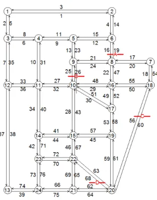
Let us consider the benchmark Sioux Falls network, which is commonly used in the trans-portation research community (cf. LeBlanc et al. [6]), to better understand the importance of a networked model. Refer to Figure1. Assume that there are four bridges, labeled as A, B, C, and D, which are vulnerable to seismic hazards.
A failure of bridge C (i.e., functional obsolescence) would detour the traffic on link 60 from node #20 to #18 to a longer path consisting of links 61, 58, 52 and 50. This may result in higher travel cost, due to detours and resulting congestion. Additionally, the varied structural deficiencies of each bridge may require the use of different materials and labor for its rehabilitation. The main challenge is then formulating strategic allocations of limited resources to the bridges before they become structurally inadequate and cause undesirable consequences to the network. A strategy solely based on the ranked structural deficiency status would not guarantee system optimality. For instance, assuming that bridge D is in a worse condition than bridge C and that resources are insufficient to support retrofitting both of them, bridge D will
Figure 1: Sioux Falls network
outrank bridge C in retrofit priority, thus possibly exposing bridge C to a higher chance of reaching the state of functional obsolescence in extreme events. This solution could be highly sub-optimal, as the failure of bridge D only affects traffic on links among nodes #20, #21 and #22 while the failure of bridge C affects traffic on links among nodes #20, #19, #17, #16, and #18. From a network perspective, bridge C would be better positioned to be retrofitted.
1.2. Relevant literature
Network-based bridge retrofitting is a general transportation network protection problem, which can be grouped into two broad categories, depending on whether bridges are treated as links [3, 5, 7] or as paths [8, 9]. The former approach formulates as maximum capacity or minimum cost network flow design problems with a focus on long-term economic effect of retrofit, whereas the latter formulates maximal covering network design problems, which are more focused on short-term emergency response or maximal coverage of population centers. From a transportation system analysis viewpoint, the transportation network protection prob-lem is essentially a network design probprob-lem (NDP), in which the upper-level probprob-lem involves optimal retrofit decisions for best social welfares (e.g., minimum retrofitting cost and travel de-lay) while the lower-level problem accounts for the behaviors of network users which normally present demand-performance equilibrium [10,11,12,13,14].
Uncertainty is naturally embedded in almost all transportation protection problems. En-gineering methods based on the wait-and-see approach [15] seek optimal solutions upon the realizations of uncertainty (in the form of scenarios), that is, the engineering methods focus on the deterministic optimization problems. The resulting scenario dependent solutions are then aggregated in order to be implemented [3, 16, 17, 18, 19]. However, since future events are unknown at the time of making decisions, scenario-specific solutions (policies) may not even be feasible for other possible scenarios. Thus, a method that can account for a large number of possible scenarios needs to be developed. Previous studies use either stochastic programming (SP) [5, 7, 20] or robust optimization (RO) method [21, 22, 23, 24] to take into account all scenarios. In general, the SP method takes the expectation of consequences of all scenarios and thus is risk-neutral and suitable for problems aiming to achieve long-term economic effects; however, it may have poor performance under extreme events. Though rare, these extreme event hazards exert severe impacts on the system. RO approach, on the other hand, considers worst-case scenario with low-occurrence probability, which may lead to too conservative and in most cases costly solutions. Therefore, neither risk-neutral SP approach nor RO-based method is best to capture the variability of risk. This motivates us to seek a new method for economic, yet robust, solutions.
In literature, a balance between risk-neutral SPs and RO is accomplished by incorporating a risk measure into the stochastic program. Such models are referred to as mean-risk SPs. The conditional value-at-risk (CVaR) is a commonly used risk measure for this purpose. It was first introduced as a risk assessment technique in portfolio management for hedging a portfolio of financial instruments to reduce risk [25, 26]. Since then, it has been applied to a number of engineering applications, such as electricity operations [27], water resources allocation [28], facility location planning [29], disaster management [30], and hazard material routing [31]. Given a probability distribution and a confidence level α, CVaR is a weighted average of value-at-risk (VaR), which is the lowerα-quantile, and the incremental values beyond the VaR cutoff point in the distribution. Thus, CVaR accounts for losses exceeding VaR. Since VaR is monotone inα, a higher confidence level leads to a more risk-averse solution. The RO problem is equivalent to considering a sufficiently largeα (worst-case scenario). CVaR has the desirable property of coherence [32,33], meaning that it is a translation invariant, subadditive, positive homogenous, monotonic function, whereas VaR is a highly nonconvex function [34]. Despite its coherence, CVaR presents some computational challenges in solving mean-risk SPs, and this has motivated numerous algorithmic developments for decomposition methods with cutting-plane approaches [28,30,35,36,37,38,39]. CVaR falls under the category of quantile risk measures, as opposed to being one of the deviation risk measures such as expected excess and absolute semi-deviation [40]. Both types of risks take into account the scenarios that exceed some pre-specified target; the former enjoys the benefit of allowing the user to specify a quantile-level of the underlying distribution as a target whereas the latter either uses the mean as the target value or requires some other scalar value to be specified for the target.
1.3. Contributions of this study
In this study, we adopt CVaR as the risk measure in developing a mean-risk two-stage stochastic programming model for transportation network protection problems, with the goal of minimizing the direct cost of retrofitting bridges in the first stage and indirect travel cost in the second stage. The first-stage decisions indicate the assignments of retrofit strategies to different bridges in an optimized manner, and are made simultaneously with second-stage traffic assignment decisions. CVaR is used to penalize scenarios with large losses using a user-specified confidence level and the risk consequence is integrated with the two-stage stochastic program with a trade-off coefficient. The model is generic and generalizable to different kinds of natural and man-made disasters.
In the context of transportation network protection, the proposed study is, to the best of our knowledge, the first study undertaken with CVaR as the risk measure. Our proposed model is closely related to the stochastic transportation protection model by Liu et al. [5], in which a central semi-deviation risk measure is used. However, our study is distinct from this prior study and advances the models in the following aspects. First, the semi-deviation measure can only capture the effects of scenarios that are worse than the expectation of second stage costs while CVaR is flexible to incorporate a spectrum of scenarios, depending on the pre-defined confidence level and the weight of the risk measure. Second, the prior studies held the assumptions of the binary damage states (i.e., either no damage or collapse) and binary retrofit strategies (i.e., retrofit or no retrofit). Although these assumptions help reduce the problem size and consequently the computational challenges associated with solving large-scale problems, this simplification may result in less informative solutions and overestimate costs. In this study, we relax the assumption by defining multiple damage states and multiple retrofit strategies based on a recent study [41] where binary decision variables are used to indicate whether a specific strategy is selected for a bridge. From the modeling perspective, it is not a trivial extension to the prior efforts due to the inherent correlations between retrofit strategies, damage states, and resulting distributions of traffic flows on the network. In addition, bridge retrofit strategies are subject to a budget limit, thereby adding to the combinatorial complexity of the problem.
The mean-risk two-stage stochastic programming model is formulated as a non-convex mixed integer nonlinear program (MINLP), wherein the travel cost for bridge links is a non-convex nonlinear function of retrofit decisions. In general, it is known that non-non-convex MINLPs can be notoriously difficult to solve [cf.42]. Thus another contribution of this study stems from the algorithmic development. In particular, we propose a decomposition that is based on the generalized Benders decomposition (GBD) method [43]. As part of this decomposition, we present a convex reformulation of the recourse function in order to resolve the issues of non-separability of first and second stage variables. This enables us to efficiently generate Benders cuts for our decomposition algorithm. We justify our model and decomposition method on a hypothetical nine-node network and then apply the model and solution method to solve a stochastic transportation network protection problem based on the benchmark Sioux Falls network (cf. Figure1). We use hazard events as a demonstration to explore the effects of risk
measures and variations in critical parameters on the optimal solutions.
The remainder of the paper is organized as follows. The mean-risk two-stage SP model is presented in section 2, followed by the convex reformulation of the recourse function in section3. Our decomposition algorithm is described in section4. Computational experiments on the two networks are carried out in section5. The paper concludes along with a discussion of future research in section6.
2. Mean-risk model
2.1. Parameters and variables
LetG= (N, A) denote a transportation network, whereN is the set of nodes andA is the set of directed arcs (or links) in the network. Denote by Rand S, for some R6=∅, S ⊂N, the set of origins and destinations in the network, respectively. The set of origin-destination (O-D) pairs is some subsetOD ⊆R×S. For every (r, s)∈ OD,drs ∈R+ is the given travel demand on traffic originating at r and ending at s. Denote by ¯A, for some ¯A 6= ∅,A¯ ⊂ A, the set of links that are subject to hazards, which mainly comprises of the at-risk bridges. The nominal traffic capacity of each link a∈ A is equal to ca. For a∈ A\A¯, it is assumed that this link capacity remains unchanged after any disastrous event (e.g., natural or man-made disasters). However, the link capacities of links in ¯A reduce due to the damage from the events and the extent of this change depends on how well the at-risk bridges were retrofitted before the events happened. The finite setH represents a list of applicable retrofit strategies for at-risk bridges in ¯A in order to mitigate the adverse impacts caused by disastrous events in the future. The set H includes the do-nothing option and each at-risk bridge can be retrofitted with exactly only one strategy. The cost of retrofitting a∈A¯with strategy h ∈H is bha. The total budget for retrofitting bridges isb0.
In this study, we consider various hazard realizations, where each realization is a prediction of damage to the structure. Let the finite set K denote the set of hazard scenarios that the network is exposed to. Each scenario k ∈ K is known to occur with a given probability pk∈(0,1). For everya∈A, h¯ ∈H, and scenario k∈K, we use the parameter θah,k ∈(0,1) to describe the ratio of post-event link capacity to the full link capacity, which can be determined externally by using bridge structural assessment, such as the study [44] for seismic damages. When disaster happens, the post-event capacity of linka∈A¯that was retrofitted with strategy h∈H is equal tocaθah,k.
We now describe the decision variables used to construct our mathematical formulation. For everya∈A, h¯ ∈H, the binary variableuha is equal to 1 if and only if linkais retrofitted by strategyh∈H. For (r, s)∈ OD,a∈Aand k∈K,xrs,ka is the flow on linkacorresponding to the traffic originating atr and terminating atsfor scenariok. The total flow on linka∈Adue to all O-D pairs is vak, and vka =P
(r,s)∈ODx rs,k
a ,∀a∈ A. In this model, we allow unsatisfied post-disaster travel demand for various reasons, such as shutdown of certain roadways, acute increased traffic congestion in the network, etc. The unsatisfied travel demand for any O-D
pair (r, s) is captured by the decision variable qrs,k and we use a big-M to impose a penalty cost for the unsatisfied demand in the objective function.
Remark 1. In the transportation network literature, traffic is often assumed to be in a user-equilibrium condition, where no traveler can further reduce their travel cost by simply changing their own routing decision [45]. This assumption holds for a normal situation, where travelers have learned and adapted to daily traffic condition. However, modeling travelers’ routing behavior in an environment following extreme events, such as earthquake, is still arguable [4]. In this paper, it is assumed that traffic flow can be controlled to achieve system-optimization and the resulting estimated travel cost can be considered as a lower bound of actual travel cost.
2.2. Two-stage stochastic models 2.2.1. Risk-neutral model
We first present a basic two-stage stochastic programming model for our problem. The first stage considers the retrofit resource allocation problem and decides the retrofitting strategy for each of the links in ¯A. Define the set U as
U := ( u∈ {0,1}|A|×|H|¯ | X h∈H uha = 1 ∀a∈A, b¯ >u≤b0 ) (1)
to include all first-stage decisions — each link in ¯Acan be retrofitted with exactly one strategy and the total budget isb0. The problem is to minimize2 b>u+EQ(u, ω). Here,b>uis the total retrofitting cost and the recourse functionQ(u, ω) is the incurred travel cost. Equivalently, the first-stage objective is to minimizeEf(u, ω), where
f(u, ω) :=b>u+Q(u, ω) (2) is the total cost function. The assumption of finitely many scenarios indexed by the set K allows us to discretize the expected travel cost function and state our two-stage stochastic program as (2-stage SP) : min u X k∈K pkfk(u) = min u b >u+X k∈K pkQk(u) s.t. u∈U, (3)
wherefk(u) =b>u+Qk(u) is the total cost function for thekthscenario, in whichQk(u) is the optimal value for the total travel cost, given the retrofitting vectoru. The recourse function is
2
based on an explicit traffic assignment model and for thekth scenario it is defined as Qk(u) = min xk,qk γ X a∈A vaktka + M X (r,s)∈OD qrs,k (4a) = min vk,qk,xk γ X a∈A t0a vak+δ (v k a)5 ˆ ck a(u)4 + M X (r,s)∈OD qrs,k (4b) s.t. vka= X (r,s)∈OD xrs,ka ∀a∈A, (xk, qk)∈X. (4c)
In the second stage,vakis the aggregation of link flow xrs,ka over all O-D pairs (r, s),qrs,k is the unsatisfied demand between an O-D pairs (r, s), and
tka=t0a " 1 +δ vak ˆ ck a(u) 4# ∀a∈A (5)
is the link travel time per unit flow. The objective function (4a) is to minimize the total cost of traffic flow on the network and consists of two terms. Each product vkatka is equal to the travel time for the entire flow on link a∈A and upon scaling this with the parameter γ that converts travel time to a monetary value3. The second term represents the “penalty cost” for unsatisfied demand. In our second stage problem, unsatisfied travel demand is penalized for economic concerns and a big positive number M is used to represent peoples’ willingness to travel. Compared to the value of time, peoples’ willingness to travel is hard to calibrate and is beyond the scope of this study; we simply use a big number to penalize the unsatisfied demand. The link travel time per unit flow is usually a non-decreasing link performance function of the aggregated link flow and a non-increasing function of the post-event link capacity in each scenario. Equation (5) expresses the dependence oftk
aonvakusing the Bureau of Public Records (BPR) function [46], in which t0a is a parameter for the free-flow-speed travel time of link a, δ is an empirical data (e.g., 0.15), and the denominator ˆcka(u), which is a function of the first stage decision u, denotes the remaining link capacity on linka in scenario k:
ˆ cka(u) = caPh∈Hθ h,k a uha a∈A¯ ca a∈A\A.¯ (6) 3
In practice, determining the value ofγ requires approximation of value of travel time savings, which is assumed to be equal to a nationwide median gross compensation for business travel (U.S. Department of Trans-portation, 2014).
The recourse functionQk(u) seeks to optimize flows over the setX, defined as: X:=n(x, q)≥(0,0)| X j: (r,j)∈A xrsrj− X j: (j,r)∈A xrsjr+qrs=drs ∀(r, s)∈ OD (7a) X j: (s,j)∈A xrssj − X j: (j,s)∈A xrsjs−qrs=−drs ∀(r, s)∈ OD (7b) X j: (i,j)∈A xrsij − X j: (j,i)∈A xrsji = 0 ∀(r, s)∈ OD, i∈N \ {r, s} . (7c)
For each O-D pair (r, s), equations (7a) and (7b) allow a slack ofqrs in the flow balance atr and s, respectively, to account for unsatisfied travel demand, whereas equation (7c) balances flow exactly at all other nodes in the network.
As the post-earthquake link capacity (6) is a linear function of retrofit decisions for links in ¯A, the decision variable u appears on the denominator of the travel time cost function in (5). This imparts non-convexity and nonlinearity to our two-stage stochastic problem and also leads to the following property.
Observation 1. Problem (2-stage SP) has complete recourse, i.e., subproblem (4) is feasible for everyu∈U.
2.2.2. Mean-risk model
We now turn to introducing our mean-risk stochastic program, which combines the two-stage risk-neutral SP model and the CVaR function for risk assessment. Recall that theα-level CVaR of a random variableZ(x, ω) is [cf.34]:
CVaRαZ(x, ω) := inf η0 η0+ 1 1−αEmax 0,Z(x, ω)−η0 =η+ 1 1−α Emax{0,Z(x, ω)−η},
where η denotes VaR. If Z(x, ω) is the first stage cost of a stochastic program, the mean-risk objective is EZ(x, ω) +λCVaRαZ(x, ω), where the coefficient λ ∈ [0,∞) represents a trade-off between the risk measure (CVaR) and the expected first stage cost. Sincef(u, ω) = b>u +Q(u, ω) is the total cost function for our problem, the mean-risk objective for us is Ef(u, ω) +λCVaRαf(u, ω). The risk-neutral problem (2-stage SP) corresponds to λ = 0. Upon discretizing with finitely many scenarios as before, performing simple manipulations arising out of translation invariance of CVaR, and linearizing the max{0,·}function in CVaR,
the mean-risk stochastic program becomes (Mean-risk SP) : min u,η,ξ (1 +λ)b >u + X k∈K pkQk(u) + λ η+ 1 1−α X k∈K pkξk ! (8a) s.t. u∈U (8b) ξk≥Qk(u)−η ∀k∈K (8c) ξk≥0 ∀k∈K, (8d)
where Qk(u) is defined by equations (4)–(6). The objective is to minimize the total cost of retrofitting bridges, expected travel cost, unsatisfied demand penalty and the risk term. Here λis a pre-defined weighting factor. A largerλvalue leans towards CVaR and thus results in a more conservative solution. On the other hand, a smallerλvalue yields a solution that weighs more on the expected cost, and thus the solution is more risk-neutral.
3. Recourse function
For each scenario k, the recourse function Qk(u) is a nonlinear optimization problem in (4). This problem is non-convex due to presence of the bilinear terms vkatka in the objective and nonlinear equality constraints definingtk
a. More importantly, since the fractional function va
ˆ ck
a(u) in (5) has u appearing linearly in the denominator, the second stage variables are
non-separablefrom the first stage variable in this formulation. Problem convexity and separability of the variables are both desirable properties of Benders-type decomposition methods for solving a two-stage stochastic program with a nonlinear second stage since they guarantee generation of valid supporting hyperplanes of the recourse function [cf.43,47]. Our decomposition algorithm for solving (Mean-risk SP) is presented in§4. In this section, we derive a reformulation ofQk(u) in (4b) that is not only a convex program for everyu∈U but also achieves separability between first and second stage variables. This reformulation leads to a convex MINLP formulation for solving (Mean-risk SP) as a single optimization problem.
For a fixed u ∈ U, the recourse value Qk(u) can be obtained by solving the convex opti-mization problem (4). However this does not tell us anything about the convexity of Qk(·). We exploit properties of the discrete setU to show that the recourse function is indeed convex. Our main approach is to eliminateu from the denominator in (4b) and make the subproblem separable in first and second stage variables. In particular, we obtain subproblem constraints that are linear inu, convex invand do not contain product terms betweenuand any ofv, q, x. There are different ways of achieving this and we present these next.
Let us introduce a auxiliary second stage non-negative continuous variableyakfor eacha∈A¯ and add the inequality
yak≥ (v k a)5 (caPh∈Huhaθ h,k a )4 ∀a∈A.¯ (9)
The right hand side of the above inequality appears in the objective (4b) with a positive coefficientγδt0a. Hence we have
Qk(u) = min vk,qk,xk,yk γ X a∈A t0a h vak+δyak i + M X (r,s)∈OD qrs,k (10a) s.t. (4c),(9). (10b)
The following lemma guides our convex reformulation forQk(u).
Lemma 1. Fora∈A¯ and u∈U, P
h∈Hθhka uha β =P h∈H θhka β uha for all β∈R. The proof is straightforward. Since P
h∈Huha = 1 and uha ∈ {0,1}, it must be that for every a∈ A¯, we have uha = 1 for some h ∈ H and uha0 = 0 for all h0 ∈ H\ {h}. Hence both (P
h∈Hθhka uha)β and P
h∈H(θhka )βuha are equal to (θahk)β.
After clearing the denominator in (9) and applying Lemma 1 withβ = 4, we obtain
(vak)5≤c4a " X h∈H θhka 4uha # yka ∀a∈A.¯ (11)
Remark 2. For u ∈ U, since P
huha = 1 and uha ∈ {0,1}, the term P
h∈H θahk 4
uha can be interpreted as the unary expansion of a discrete variable that takes values in the finite set
∪h{ θhka 4}. The right hand side of inequality (11) is then the product of a discrete variable and a non-negative continuous variable and is therefore a bilinear term. Another formulation for this bilinear term can be obtained using the binary expansion of the discrete variable, where only log2|H|many {0,1}variables (as opposed to |H| {0,1} u’s in the unary case) are required. Gupte et al. [48] theoretically compared unary and binary expansion reformulations for bilinear optimization problems, obtained new valid inequalities to strengthen the continuous relaxation of the binary reformulation and showed that these convexifications work well on hard test instances. This encourages the use of binary expansion formulations for general bilinear problems. However, in our case since the cardinality of H is quite small (e.g., 5), the discrete variable takes only up to 5 different values and there is no significant benefit of adopting the logarithmic formulation for ∪h θhka
4
. Therefore we choose to not modify the termP
h∈H θhka 4
uha in (11).
In mixed integer nonlinear optimization literature, it is common practice to replace each nonlinear constraint of≤-type with the convex envelope of the corresponding nonlinear func-tion; see Tawarmalani and Sahinidis [49]. Such a replacement usually relaxes the nonlinear constraint, although if some of the variables are discrete, one may sometimes also obtain an exact reformulation of the constraint. The≤-inequality in (11) has different sets of variables on the left and right hand sides. Therefore, if we write the constraint as the difference of the left and right hand sides, taking the convex envelope of this difference is equivalent to separately taking the convex envelope of the left hand side and the concave envelope of the right hand
side. The left hand side in (11) is a univariate convex function of va overR+ and hence does not require any convexification. For the right hand side, we have a bilinear term between a discrete variableP h∈H θhka 4 uh a∈ ∪h n θhk a 4o
(cf. Remark 2) and a continuous variableyk a. The concave envelope of this bilinear term is given by its McCormick inequalities [50], which depend on lower and upper bounds on the variables appearing in the bilinear term. The bounds forP
h∈H θhka 4
uha and yak can be obtained as follows. It is clear that for u∈U,
θka ≤ X h∈H θahk4uha≤θ¯ak, where θka:= min h∈H θ hk a 4 , θ¯ka:= max h∈H θ hk a 4 .
From equations (4c) and (9) we get the lower bound on yka to be zero. For every a∈ A¯, let ςa > 0 be a large enough positive constant such that every optimal solution to (10) satisfies va≤caςa ∀a∈A¯. Then by inequality (9) and Lemma1, every optimal solution to (10) satisfies
yak≤ caς 5 a P h(θahk)4uha (12a) which leads to yka≤ caς 5 a θka (12b)
since u ∈ U. Using these lower and upper bounds, the McCormick concave envelope of the bilinear term on the right hand side of (11) is
c4amin ( ¯ θakyak, θkayak + caς 5 a θka X h∈H θahk 4 uha − caςa5 ) . (13)
and hence we have two inequalities for (11):
(vak)5 ≤c4aθ¯akyak, (vak)5 ≤c4aθkayak + (caςa) 5 θka X h∈H θhka 4uha − (caςa)5 ∀a∈A.¯ (14)
Gupte et al. [48, Proposition 2.1] tells us that modeling a bilinear term between a general integer and a continuous variable with the McCormick inequalities allows for more integer solutions. The same holds true when the bilinear term is between a general discrete and a continuous variable. Therefore (14) yields a relaxation but not a reformulation of (11). Although this relaxation can be used to under-estimate the recourse functionQk(u), doing so will only yield weaker cuts in the decomposition algorithm.
to (11) if and only if there exists some wka such that (vka)5 ≤ c4awka, (15a) 0≤wak≤ caςa5, wka ≤ " X h∈H θhka 4uha # yak. (15b)
This equivalence is correct because 0 ≤ va ≤ caςa implies that the left hand side of (11) is upper-bounded by (caςa)5. Since caςa5 < caςa5θ¯ka/θka and the right hand side is the product of the upper bounds onP
h∈H θhka 4
uha andyak, respectively, it is clear that the upper bound on wak is nontrivial. We will convexify (15b) to obtain a strong reformulation of (11).
Remark 3. Inequalities (14) are precisely the projection of the McCormick relaxation of
va5≤c4awka, 0≤wak≤ " X h∈H θahk 4 uha # yka, (16)
where the bilinear term is relaxed using (13). Observe that (15) and (16) are each equivalent to (11) but (16) is a relaxation of (15) in the (vka,(uha)h, yak, wak)-space. Therefore convexifying (15b) produces a stronger reformulation in the (vak,(uah)h, yak, wak)-space than convexifying 0≤ wk a ≤ h P h∈H θahk 4 uh a i yk
a in (16) and hence could lead to stronger cuts in the decomposition algorithm.
Equation (15b) represents a bounded product term between a discrete and a continuous variable and for such bilinear terms, we note that the McCormick envelopes are neither a reformulation nor do they yield the convex hull.
Observation 2. DenoteI :={b1,b2, . . . ,bm}×[0,d]×[0, η]withm≥3,0≤b1<b2 <· · ·<bm and η <bmd. Let R:={(x,y, ν)∈ I |ν ≤xy}, M:={(x,y, ν)∈ I |ν ≤bmy, ν ≤b1y+dx −
db1} be the McCormick relaxation of R, and M0 := {(x,y, ν) ∈[b1,bm]×[0,d]×[0, η] |ν ≤
bmy, ν ≤b1y+dx −db1} be the continuous relaxation of M. Then R(Mand convR(M0.
Proof. Mbeing the McCormick relaxation of Rleads toR ⊆ M and convR ⊆ M0. Denote
χ0:= d
η(1− b1
bm)
, χ1:=ηmin{1,(b2−b1)χ0}.
Then (b2,χbm1, χ1)∈ M \ R. Note that (b1+χ10,bηm, η) is an extreme point ofM0. Suppose this point can be written as a nontrivial convex combination of finitely many (xt,yt, νt)∈ R. Then νt =η ∀t. Since νt ≤xtyt and xt ≤ bm, it follows that yt ≥ η/b
m and hence yt = η/bm and
xt = bm for all t. Consequently, b1+χ10 = bm, which is a contradiction because η < bmd by assumption.
discrete variables. Letν =P
ibiziwith P
izi= 1,zi ∈ {0,1} ∀i. Then disjunctive programming [51] implies that convR is equal to the projection onto the (x,y, ν)-space of the polyhedron
n (x,y, ν,z)| x = m X i=1 bizi, ν= m X i=1 νi, y= m X i=1 yi 0≤yi≤dzi, 0≤νi≤δzi, νi≤biyi ∀i m X i=1 zi = 1, zi ≥0 ∀i o . (17) Since P
h(θhka )4ua is the unary expansion of a discrete variable as mentioned in Remark 2, we may apply (17) directly to (15b). However, we will first strengthen the bounds on the yk
a variables in each disjunction. Of the two upper bounds on yka in (12a) and (12b), the former is stronger but is a function of u whereas the latter is weaker but is a constant. The constant bound in (12b) is necessary for deriving McCormick relaxations of bilinear terms as in Observation2. The bound in (12a) can be incorporated into the disjunctive programming approach of equation (17). Since yka ≤ caςa5
P
h(θahk)4uha by equation (12a) and
P
huha = 1 and uha ∈ {0,1} ∀hfor everyu∈U, it is clear that convexifying (15b) is equivalent to convexifying the following finite union of polytopes:
[ h∈H (ua, yka, wka)|ua=eh, 0≤yak≤ caςa5 (θhk a )4 , 0≤wka≤caςa5, wak ≤c4a(θahk)4yak . (18)
where eh is the hth coordinate unit vector. A straightforward application of disjunctive pro-gramming [51] gives us the convex hull of (18), and hence that of (15b), thereby resulting in a strong reformulation of the recourse function, which we state next.
Proposition 1. The recourse function of thekth scenario can be formulated as:
Qk(u) = min vk,qk,xk yk,wk γ X a∈A t0a h vak+δyak i + M X (r,s)∈OD qrs,k (19a) s.t. vak= X (r,s)∈OD xrs,ka ∀a∈A, (xk, qk)∈X (19b) (vka)5 ≤c4aX h∈H wahk, yka= X h∈H yhka ∀a∈A¯ (19c) wahk≤c4a(θahk)4yahk ∀h∈H, a∈A¯ (19d) 0≤yhka ≤ caς 5 a (θhk a )4 uah, 0≤wahk≤caςa5uha ∀h∈H, a∈A¯ (19e)
on the traffic volume of link a.
Notice that Proposition1linearly separates the first stage variableu from the second stage variables. This implies that the recourse functionQk(u) is convex inuand can be approximated by supporting hyperplanes. It also implies a convex MINLP formulation for the mean risk problem (8).
(Convex MINLP) : min u,η,ξ v,q,x,y,w (1 +λ)b>u + X k∈K pk γ X a∈A t0a h vak+δyka i + M X (r,s)∈OD qrs,k +λ η+ 1 1−α X k∈K pkξk ! s.t. u∈U, ξk≥0 ∀k∈K ξk≥γ X a∈A t0a h vka+δyaki + M X (r,s)∈OD qrs,k − η ∀k∈K (19b)−(19e) ∀k∈K
This convex MINLP can be solved to-optimality using state-of-the-art MINLP solvers. How-ever we demonstrate in §5 that even on a simple nine-node network, these generic global optimization solvers take a long time to converge, thereby making this approach intractable for larger-sized practical instances. This motivates our algorithmic approach in the next section.
4. Decomposition method
Extensive algorithmic efforts have been made to improve the efficiency of solution algorithms for MINLPs, including the widely used branch and bound [52] with its variants — LP/NLP based branch and bound method [53] and spatial branch and bound [54], as well as Generalized Benders Decomposition (GBD) method [43]. The branch and bound method is an implicit enumeration procedure and can be computationally expensive when the number of integer variables is large. The GBD, on the other hand, can be effective in handling computationally challenging MINLPs by decomposing them to smaller tractable subproblems. In this study, we apply a decomposition method based on GBD. Also note that there are other plausible solution methods, including Extended Cutting Plane method [55], and outer approximation [56]. Though beyond the scope of this study, comparisons between these different methods in terms of solution quality and performance are worthy of investigation in future works.
The mean-risk SP model (8) is decomposed into a master problem and one subproblem for each scenariok. The master problem is a mixed 0\1 linear program (MILP) and contains first-stage integer variablesu and the value-at-risk η. The sub-problems are evaluated for the second-stage cost, given the first-stage variableu. Combined with the first-stage cost, we can compute CVaR for the overall cost at the optimum of the master problem. We will discuss the details of our decomposition method in this section.
GBD was proposed by Geoffrion [43] and a detailed exposition on it can be found, for ex-ample, in Floudas [47]. In this method, when the first stage variables are temporally held fixed, the remaining optimization problem is considerably more tractable than the original one. As for this study, if bridge retrofit decision variableuand the value-at-riskηare temporarily fixed, the remaining problem (4) becomes a traffic assignment problem based on system-optimization condition, which may be effectively solved by using commercial nonlinear program solvers. The CVaR value can be obtained once we have travel cost function values from the traffic assignment problems corresponding to different scenarios.
In the objective function of the master problem, the recourse function travel cost and CVaR are not known explicitly in advance. Thus, two optimality cuts are added iteratively to approximate them. At iteration i, let πkiu ≥π0ki be a cut that lower approximates Qk(u). Then the master problem at any iterationl reads as
(Master) : min u,η,ξ,φ1 (1 +λ)b>u+φ1+λ η+ 1 1−α X k∈K pkξk ! s.t. u∈U, ξk≥0 ∀k∈K Optimality cut 1 φ1≥ X k pk(πkiu−π0ki) i= 1,2, . . . , l Optimality cut 2 ξk≥πkiu−π0ki−η ∀k∈K, i= 1,2, . . . , l
The exact forms of these optimality cuts are presented in Proposition2. According to Obser-vation1, the general problem hascomplete recourse and the feasibility cut constraint can thus be omitted.
Let (¯u,η,¯ ξ,¯φ¯1) be an optimal solution to the master problem. If ¯φ1 <
X
k∈K
pkQk(¯u), then
optimality cut 1 will be added to the master problem. IfP
k∈Kpkξ¯k<Pk∈Kpkmax{0, Qk(¯u)− ¯
η}, then optimality cut 2 will be added to the master problem. These optimality cuts are generated using Lagrange multipliers for each subproblem, which is a convex nonlinear problem, withu fixed to ¯u. (Subproblem k) :Qk(¯u) = min vk,qk,xk yk,wk (19a) s.t. constraints (19b)−(19d) 0≤yahk≤ caς 5 a (θhk a )4 ¯ uah, 0≤wahk≤caςa5u¯ha ∀h∈H, a∈A¯
The convex reformulation of Qk(u) in Proposition 1 and the arguments thereafter imply that it is straightforward to apply the GBD method for generating optimality cuts in the master problem.
Proposition 2. Letu¯l be an optimum solution of the master problem atlth iteration. For each scenario k, let µkl and λkl be vectors of optimum Lagrange multipliers for the last two sets of constraints in subproblem Qk(¯ul). Denote
¯ yahk:= caς 5 a (θhk a )4 h∈H, a∈A.¯
Then the optimality cuts for the lth iteration are:
φ1 ≥
X
k∈K
pk[Qk(¯ul)−µkly¯k(u−u¯l)−λklcaς5(u−u¯l)] (20a)
ξk≥ Qk(¯ul)−µkly¯k(u−u¯l)−λklcaς5(u−u¯l)−η ∀k∈K (20b)
Proof. Proposition1linearly separates the first stage variableufrom the second stage variables, i.e., the subproblem constraints in (19e) are the only ones containing both first and second stage variables and these can be represented ash1(u) +g1(w)≤0 or h2(u) +g2(y)≤0 where
h1, h2, g1, g2 are all linear functions. This structure fits in with the so-called P-property of GBD [cf.47,§6.3.5.1], allowing for a straightforward application of GBD and thereby leading to the proposed optimality cuts.
Multiple optimality cuts may help improve algorithm efficiency. Readers may refer to Birge and Louveaux [15] for details. The multi-cut version of optimality cut for (20a) is
φk1 ≥Qk(¯ul)−µkly¯k(u−u¯l)−λklcaς5(u−u¯l) (21) Accordingly, we should use the aggregation of cuts P
k∈Kpkφk1 to replace φ1 in the objective function of (Master). Note that due to the CVaR function definition, optimality cut (20b) is already in multi-cut version. In each iteration, there are|K|+1 constraints added to the master problem, consisting of|K|constraint (20b) and one constraint (20a).
The decomposition algorithm procedure:
1. Initializationl= 0.
2. Solve (Master). Let (¯u,η,¯ ξ,¯φ¯1,φ¯2) be optimal solution and set ¯φ= ¯φ1+λ(¯η+1−α1 Pkpkξ¯k). 3. Fixu= ¯u and solve (Subproblem k) for all k∈K. Setl=l+ 1 and calculate
φ∗ = X k∈K
pkQk(¯u) +λCVaRαQ(¯u).
4. The procedure terminates if the optimality gap|1− φ¯
φ∗| ≤(is a predefined small value) is met. Optimal solution is found. Otherwise, add optimality cuts (20a) (or the multi-cut version (21)) and (20b) to the master problem, and go back to step 2.
5. Numerical examples
The proposed mean-risk model and decomposition methods are first validated using a hypo-thetical small nine-node network. The Sioux-Falls network is then used to explore the impacts of uncertainty, network topology, and critical parameters on the strategic decisions on highway bridge retrofits. All instances were programmed in AMPL. For our decomposition, the master problem was solved as a MILP with CPLEX and with the multi-cut version of optimality cuts, and each subproblem was solved as a convex nonlinear program with CONOPT.
5.1. Nine-node network
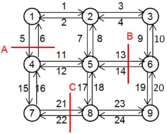
The nine-node network is shown in Figure2. It consists of nine nodes, 24 directional links, and 72 (= 8×9) O-D pairs. Assume that three bridges on both directions on the network, labeled as A, B, and C, are vulnerable to seismic disasters and their post-disaster capacities may be reduced while other road links are assumed intact. The nine-node instances were tested on a desktop with 8 GB RAM and Intel Core [email protected] processor under Windows 7 environment.
Figure 2: Nine-node network
The parameter θh,ka is the ratio of bridge remaining capacity to the full capacity, which depends on the specific scenario, location of the bridge, and the retrofit strategies applied. Five strategies, denoted as h0 – h4, are considered. The “do nothing” strategy is h0 and a higher index indicates a more robust, and hence more costly, strategy. In this experiment, we randomly generated θh,ka ∈(0,1] while ensuring that a higher numbered strategy results in a higher value ofθh,ka . As a demonstration, Table1reports the ratios for one scenario. The initial values for all second-stage variables are set to be zero. The initial solution for the first-stage decision variableu is set as follows: for every a ∈A¯, uh0
a = 1 and uha = 0 for h 6= h0. Other critical parameters are: α= 0.7, γ= 1000, λ= 1, andy= 1000.
Two recent papers [57, 58] demonstrate that commercial MINLP solvers can successfully solve nonlinear, discrete transportation problems. We obtained benchmark solutions by us-ing two commercial solvers — BONMIN [59] and FilMINT [60], to justify our decomposition method by using the small-scale network. We tested the model using four different sizes of scenario sets. In each set, scenarios are randomly generated to create variations in uncertainty realizations in order to justify the effects of CVaR.
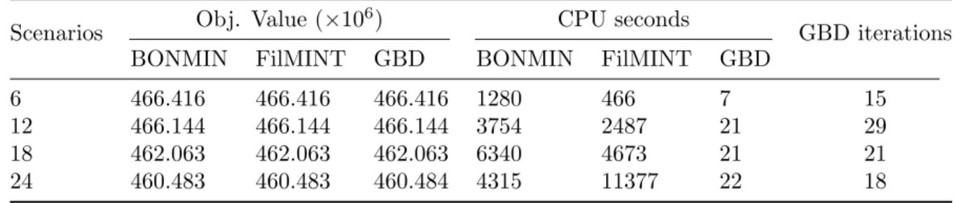
Table 2 compares optimal objective values and solution times for the MINLP solvers and our decomposition algorithm (column GBD). As is to be expected, the objective values are almost identical for all three methods. The solution times using GBD are always substantially smaller than those using BONMIN and FilMINT. One may also notice that the increase in the number of scenarios does not necessarily translate to more GBD iterations. With more scenarios, more sub-problems need to be solved in each iteration, thereby GBD takes longer total time to finish. This explains why the solution time for GBD is almost identical when solving 12, 18, 24 scenarios even though the number of iterations was smallest in the case of 24 scenarios compared to the 12 and 18 scenarios. The experimental results in Table2justify the use of our proposed decomposition for large scaled problems, such as the Sioux Falls network.
Table 1: Sample values ofθh,ka for a fixed scenariok.
Link Strategy h0 h1 h2 h3 h4 link5 0.05 0.5 0.5 0.5 1 link6 0.05 0.5 0.5 0.5 1 link13 0.5 0.5 0.5 0.75 0.75 link14 0.5 0.5 0.5 0.75 0.75 link21 0.17 0.33 0.33 0.67 0.67 link22 0.17 0.33 0.33 0.67 0.67
Table 2: Comparisons between GBD and MINLP solvers withα= 0.7, λ= 1.
Scenarios Obj. Value (×10
6) CPU seconds
GBD iterations BONMIN FilMINT GBD BONMIN FilMINT GBD
6 466.416 466.416 466.416 1280 466 7 15 12 466.144 466.144 466.144 3754 2487 21 29 18 462.063 462.063 462.063 6340 4673 21 21 24 460.483 460.483 460.484 4315 11377 22 18
5.2. Sioux Falls network
The Sioux Falls network in Figure1consists of 24 nodes, 76 links, and 552 O-D pairs. The trip demands between all O-D demands are adopted from [6]. We adopted critical parameters from Fan et al. [7], including the peak 2-hour conversion valueγ = 2400 to convert peak 2-hour delay to a monthly monetary value loss, which is set as 8×30×10 = 2400, where 8 is the daily adjust factor with 30 days duration and 10 is the value of travel time savings for drivers. We used = 0.5% for optimality gap tolerance to terminate the GBD algorithm. The instances were programmed in AMPL and run on a Linux cluster node with 16 Intel Cores and a total 64 GB RAM.
An engineering method to estimate earthquake damage of structures uses discrete damage states [61]; that is, the residual post-earthquake capacity ratio θah,k has discrete values. There are currently no publicly-available datasets for estimating the post-earthquate damage states for a given road network. Because collecting such data is beyond the scope of this study, we randomly generated θah,k such that there are substantial variations among different scenarios to justify the use of stochastic programming method in our study.
That being said, we develop a simple mechanism to generate θah,k in two steps. First, we consider three levels of damages, which are low, medium, and high damages and assume that the damages to the bridges at risk are independent. For a low-damage scenario k, we select five values for θh,ka at random from {1/N,2/N, . . . ,(N −1)/N,1} (we used N = 6 in this study). For medium and high damage scenarios, we pick five numbers randomly from
{1/N,2/N, . . . ,(N−1)/N}and{1/N,2/N, . . . ,(N−2)/N}, respectively. Note thatθah,k under a low-damage scenario has larger range of numbers to choose from than θah,k under medium and high damage scenarios. Statistically, bridge residual capacity under high-damage scenarios is lower than that under low-damage scenarios for the same bridge. However, due to the complexity involved in the estimation, such as locations and structures of different bridges, there are inevitable fluctuations in the residual capacities, which are captured in our scenario generation mechanism. Also, for any bridgea under scenariok, the θh,ka value should be non-decreasing with an enhanced (i.e., higher numbered strategy) strategy h, i.e., θhi+1,k
a ≥ θahi,k for i= 0, . . . ,3. Based on this, we assign the selected five numbers for θh,ka according to the different retrofit strategies. We also assume that the occurrences of the three categories of scenarios follow a predefined ratio. For example, if a ratio of 5:3:2 is assumed for low-, median-and high-damage scenarios, respectively, for a total of 20 scenarios, the occurrences of each category of scenarios will be 10, 6, 4, respectively. The probabilities associated with scenarios are randomly generated from a uniform distribution.
We adopted the same five-strategy scheme (i.e., h0 – h4) and initial value settings from the nine-node network example. Since the Sioux falls network is much larger in size than the hypothetical nine-node network from section5.1and the experiments in Table 2 convinced us of the superiority of a decomposition approach over MINLP solvers, we obtained results using only our GBD method. Next, we explore the impacts of uncertainty, network topology, and critical parameters on the retrofit strategies from our numerical experiments.
5.2.1. Effects of risk parametersλ, α and scenarios K
The parameters α and λ reflect the decision makers’ risk preferences. We tested α= 0.7, 0.8, 0.9 and 0.95 andλ= 0.1, 0.5, 1, and 100 withy = 1500 for 20, 50, and 100 scenarios. The time limit was set to 24 hours. The confidence level parameterα controls the set of scenarios to be considered while the coefficientλweighs the CVaR in the integrated mean-risk stochastic model. Through the numerical experiments, we intend to (i) understand the effects of risk parameters on system costs; and (ii) highlight the modeling insights of a risk (i.e., CVaR) integrated stochastic program compared to a risk-neutral stochastic model.
Let us first investigate the breakdown of the total cost plotted in Figure 3 based on the result of 20 scenarios. For the purpose of this illustration, we experimented with ten different values for α. The total mean-risk cost or objective value is the sum of total expected costs and weighted CVaR. The total expected cost can be further decomposed into the retrofit cost and the expected travel cost. The impacts of the risk parameters on the cost effectiveness and CVaR will be discussed separately. Note thatαrepresents the risk preference, which quantifies the mean value of the worst (1−α)% of the total costs. In Figure 3a, CVaR increases as α increases as per the definition, i.e., a larger value of α accounts for larger realizations of the total cost, while decreasing asλ increases. The total expected cost shown in Figure 3b is comprised of the retrofit cost in Figure3cand the expected travel cost in Figure3d. The results show that increasing bothλand αgenerally increases retrofit cost, because it results in a more risk-averse policy with enhanced and more costly retrofit strategies. As a result, we expect a reduced expected travel cost, which implies a lower post-disaster capacity loss. However, the total expected cost, which is a combined retrofit and expected travel cost, is generally higher with a higherα. The retrofit cost contributes roughly 14.6%- 20% to the total expected cost.
We are also interested in understanding the managerial insights on the integration of risk assessment into a traditional risk-neutral two-stage SP model. Table 3 compares the results of our mean-risk model with the counterparts of the two-stage SP model (first row in the table). It provides some interesting insights. First, the total expected costs of mean-risk models are equal or only trivially larger than the result of two-stage SP model even when there is a discernible increase in retrofit cost. It means that the mean-risk model can hedge against larger losses at a reasonable low total expected cost. Second, the lowest travel cost of $285.338M is $25.1M(=310.437-285.338) or 8% lower than the two-stage SP model, while it costs $29 (=87-58) or 50% more in retrofit. This implies that reducing travel cost is costly. From a system-cost perspective, achieving the lowest network-wide travel cost may not be the most economical solution.
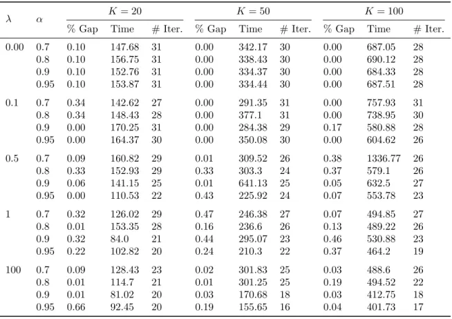
We also conducted comparisons between three different sizes of scenario sets for the same four bridges. The results and solution performances are represented in Tables 4 and 5. A larger scenario set corresponds to a larger problem size and because of our scenario generation mechanism, also has a larger number of high-damage scenarios. Between scenarios, CVaR value changes by a small extent in general. On the other hand, solution times (given in minutes) experience more noticeable changes, roughly doubling between scenarios. This is to be expected because the running time for each iteration of a non-parallelized decomposition algorithm is
(a)CVaRαf(u) (b) Total exp. costEf(u)
(c) Retrofit costb>u (d) Exp. travel costEQ(u)
Table 3: Comparisons between Risk-neutral and Mean-risk two-stage SP for 50 scenarios. The four cost columns are for total CVaR, total expected cost, retrofit cost, and expected travel cost.
λ α Cost (×10 6) Retrofit Strategy CVaRαf Ef b>u EQ A B C D 0 0.7 410.502 368.437 58 310.437 3 3 2 2 0.8 419.683 368.437 58 310.437 3 3 2 2 0.9 435.398 368.437 58 310.437 3 3 2 2 0.95 447.975 368.437 58 310.437 3 3 2 2 0.1 0.7 410.502 368.437 58 310.437 3 3 2 2 0.8 419.683 368.437 58 310.437 3 3 2 2 0.9 435.398 368.437 58 310.437 3 3 2 2 0.95 447.975 368.437 58 310.437 3 3 2 2 0.5 0.7 407.472 369.646 76 293.646 4 3 2 2 0.8 413.893 369.646 76 293.646 4 3 2 2 0.9 424.954 369.646 76 293.646 4 3 2 2 0.95 426.484 372.338 87 285.338 4 3 3 2 1 0.7 409.03 370.828 71.5 299.328 4 3 2 1 0.8 413.893 369.646 76 293.646 4 3 2 2 0.9 424.954 369.646 76 293.646 4 3 2 2 0.95 426.484 372.338 87 285.338 4 3 3 2 100 0.7 407.472 369.646 76 293.646 4 3 2 2 0.8 413.893 369.646 76 293.646 4 3 2 2 0.9 420.096 373.841 78 295.841 4 3 3 0 0.95 424.233 373.494 82.5 290.994 4 3 3 1
roughly proportional to the number of scenarios involved in the problem. Note that each of the 100 scenario instance takes at least 7 hours to solve within 0.5% gap, and one of them (λ= 0.5, α= 0.7) takes more than 22 hours.
To test the limits of performance of our GBD method, we also experimented with 200 scenarios. On all of these instances our method had more than 20% gap after the 24 hour time limit, and because no additional insight was gained from the output, we do not include these numbers in our tables. This indicates that the current implementation of our decomposition does not scale well to 200 or more scenarios. In practice, the scenario set of a network protection problem is estimated using the intuition provided by structural engineers who are able to somewhat reasonably predict the various hazard realizations and their corresponding damage to the network. Consequently, these problems typically tend to have less than 200 scenarios. However, this may not always be true and some applications may require modeling with a large scenario set. Also, a larger number of scenarios provides a better representation of the randomness. If indeed one wishes to solve the problem with|K| ≥200, either due to practical application or to have the random variables in the model be as close to having a continuous probability distribution as possible, then alternate and more efficient implementations must be sought. We offer some ideas on this in the next section. That being said, we emphasize that a decomposition approach is still preferred over solving the entire discretized problem as a MINLP; this assertion was reaffirmed by trying to solve the 200 scenario instances with a MINLP solver and observing that the solver crashed on most of them or had extremely high gaps after 24 hours.
6. Summary and future work
We formulated a mean-risk MINLP for transportation network protection (e.g., retrofitting highway bridges) hedging against extreme disasters (e.g., earthquakes) on a system level, where CVaR is considered as the risk measurement and integrated into the optimization framework. This is the first study that explicitly considers CVaR as the risk measure in the field of trans-portation network protection. The mean-risk formulation is a nonconvex MINLP, but we show that the recourse function can be reformulated to be convex in the bridge retrofit variables, which appear as first stage decisions. This leads to the development of a Benders-type decom-position algorithm to solve the MINLP.
We demonstrate the mean-risk model and decomposition method using two numerical ex-amples: (i) a small nine-node network used to validate the proposed decomposition method and exhibit its superior performance in comparison to standard MINLP software; (ii) the benchmark Sioux Falls network to explore the correlations between risk parameters and retrofit decisions and their impacts on the system costs. We investigated the capacity of our solution method in handling different sized scenario sets and also compared the results of our mean-risk model with the risk-neutral model to understand the costs and effects of using a more risk-averse model. From the results, there are several worthy notes. First, by using a weighted mean-risk criterion, the mean-risk model hedges against larger losses where the two risk coefficients reflect
Table 4: Total expected and CVaR costs (×106
) under different number of scenarios.
λ α K= 20 K= 50 K= 100 CVaRαf Ef CVaRαf Ef CVaRαf Ef 0 0.7 399.143 365.798 410.502 368.437 417.665 370.661 0.8 408.018 365.798 419.683 368.437 430.958 370.661 0.9 426.197 365.798 435.398 368.437 453.774 370.661 0.95 438.264 365.798 447.975 368.437 482.858 370.661 0.1 0.7 399.143 365.798 410.502 368.437 417.665 370.661 0.8 408.018 365.798 419.683 368.437 418.16 371.612 0.9 426.197 365.798 435.398 368.437 430.395 371.612 0.95 438.264 365.798 447.975 368.437 439.092 371.612 0.5 0.7 399.143 365.798 407.472 369.646 409.375 371.612 0.8 408.018 365.798 413.893 369.646 418.16 371.612 0.9 409.962 370.116 424.954 369.646 425.02 373.346 0.95 412.771 370.116 426.484 372.338 431.136 373.346 1 0.7 399.143 365.798 409.03 370.828 408.011 373.346 0.8 401.749 369.721 413.893 369.646 416.344 373.346 0.9 410.505 369.721 424.954 369.646 425.461 374.152 0.95 412.771 370.116 426.484 372.338 428.039 374.875 100 0.7 396.316 370.116 407.472 369.646 408.011 373.346 0.8 401.749 369.721 413.893 369.646 416.55 374.152 0.9 407.975 375.106 420.096 373.841 423.003 374.875 0.95 410.876 375.106 424.233 373.494 428.039 374.875
Table 5: Solution performances under different number of scenarios. Gap refers to optimality gap. Times are in minutes.
λ α K= 20 K= 50 K= 100
% Gap Time # Iter. % Gap Time # Iter. % Gap Time # Iter.
0.00 0.7 0.10 147.68 31 0.00 342.17 30 0.00 687.05 28 0.8 0.10 156.75 31 0.00 338.43 30 0.00 690.12 28 0.9 0.10 152.76 31 0.00 334.37 30 0.00 684.33 28 0.95 0.10 153.87 31 0.00 334.44 30 0.00 687.51 28 0.1 0.7 0.34 142.62 27 0.00 291.35 31 0.00 757.93 31 0.8 0.34 148.43 28 0.00 377.1 31 0.00 738.95 30 0.9 0.00 170.25 31 0.00 284.38 29 0.17 580.88 28 0.95 0.00 164.37 30 0.00 350.08 30 0.00 604.62 26 0.5 0.7 0.09 160.82 29 0.01 309.52 26 0.38 1336.77 26 0.8 0.33 152.93 29 0.33 303.3 24 0.37 579.1 26 0.9 0.06 141.15 25 0.01 641.13 25 0.05 632.5 27 0.95 0.00 110.53 22 0.43 225.92 24 0.07 553.78 23 1 0.7 0.32 126.02 29 0.47 246.38 27 0.07 494.85 27 0.8 0.01 153.35 28 0.16 236.6 26 0.13 489.22 26 0.9 0.32 84.0 21 0.44 295.07 23 0.46 530.88 23 0.95 0.22 102.82 20 0.24 210.3 22 0.37 464.2 19 100 0.7 0.09 128.43 23 0.02 301.83 25 0.03 488.6 26 0.8 0.01 114.7 21 0.01 301.25 25 0.19 494.52 22 0.9 0.01 81.02 20 0.03 170.68 18 0.03 412.75 18 0.95 0.66 92.45 20 0.19 155.65 16 0.04 401.73 17
decision makers’ risk preferences. It has a slightly larger total expected cost (retrofit cost plus travel cost) than the two-stage SP model and there is a discernible increase in retrofit cost and decrease in travel cost. Second, there are quite a few duplicated solutions with different combinations of risk parameters.
Several future directions involving both the modeling and algorithmic part would be worthy research efforts. From a modeling perspective, incorporating traffic equilibrium to model route choices of network users seems relevant. This will make the model a Mathematical Program with Equilibrium Constraints (MPEC). One of the challenges would be converting this MPEC to a MINLP through regularization or penalization. Once it is in the form of MINLP, we may apply the developed decomposition method for obtaining solutions. In addition, more realistic assumptions on post-disaster traffic capacity (i.e.,θka) may be included by integrating the network model with structural analysis. The structural analysis that relates the bridge performance with retrofit strategies that cost differently may produce a nonlinear bridge traffic capacity-cost relationship. Instead of assuming a constant or linear relationship as in most optimization-based transportation network protection problems, we could use finite element analysis to construct a structural performance-retrofit level relationship between the structural strength and allocated budget for each bridge. Lastly, one may also consider modeling with more general quantile risk measures and empirically comparing the solutions obtained from different risk measures.
Several enhancements can be explored on the algorithmic side to obtain a more sophisticated method that achieves faster convergence on problems with large number of scenarios. First, the subproblems can be solved in parallel at each iteration. Second, the decomposition can be implemented via a one-tree approach where a single branch-and-cut tree is maintained for the master problem and at each integer feasible node of this tree, subproblems are solved to generate globally valid optimality cuts. The choice of modeling and optimization software in this paper present a handicap with respect to these two extensions, and hence alternate implementations must be adopted. Third, alternate convex reformulations of the recourse function deserve attention. These may lead to stronger cutting planes for each scenario. Finally, this paper proposed a Benders-type (also called primal) decomposition algorithm; a natural extension would be a dual (also called scenario) decomposition algorithm which would require different convexification techniques.
Acknowledgement
The authors would like to thank two referees whose meticulous reading and constructive suggestions contributed to improving this manuscript. The second author (AG) was partially supported by ONR grant N00014-16-1-2725.
References
[1] I. Buckle, I. Friedland, J. Mander, G. Martin, R. Nutt, M. Power, Seismic retrofitting manual for highway structures: Part 1–Bridges, Technical Report, US Department of Transportation, Federal Highway Administration, 2006.
[2] ASCE, 2013 Report Card for America’s Infrastructure, American Society of Civil Engi-neers, 2013.
[3] L. Chang, F. Peng, Y. Ouyang, A. Elnashai, B. Spencer, Bridge seismic retrofit pro-gram planning to maximize postearthquake transportation network capacity, Journal of Infrastructure Systems 18 (2012) 75–88.
[4] Y. Fan, C. Liu, Solving stochastic transportation network protection problems using the progressive hedging-based method, Networks and Spatial Economics 10 (2010) 193–208. [5] C. Liu, Y. Fan, F. Ord´o˜nez, A two-stage stochastic programming model for transportation
network protection, Computers & Operations Research 36 (2009) 1582–1590.
[6] L. J. LeBlanc, E. K. Morlok, W. P. Pierskalla, An efficient approach to solving the road network equilibrium traffic assignment problem, Transportation Research 9 (1975) 309– 318.
[7] Y. Fan, C. Liu, R. Lee, A. S. Kiremidjian, Highway network retrofit under seismic hazard, Journal of Infrastructure Systems 16 (2010) 181–187.
[8] A. S. Mohaymany, N. Pirnazar, Critical routes determination for emergency transportation network aftermath earthquake, in: 2007 IEEE International Conference on Industrial Engineering and Engineering Management, IEEE, 2007, pp. 817–21.
[9] K. Viswanath, S. Peeta, Multicommodity maximal covering network design problem for planning critical routes for earthquake response, in: Transportation Research Board 82nd Annual Meeting, Transportation Research Record, National Research Council, 2003, pp. 1–10.
[10] A. Nagurney, On the relationship between supply chain and transportation network equi-libria: A supernetwork equivalence with computations, Transportation Research Part E: Logistics and Transportation Review 42 (2006) 293–316.
[11] A. Nagurney, Mathematical models of transportation and networks, in: W.-B. Zhang (Ed.), Mathematical Models in Economics, volume II, Encyclopedia of Life Support Sys-tems, 2007, pp. 346–384.
[12] M. Patriksson, The traffic assignment problem: models and methods, VSP, The Nether-lands, 1994.
[13] S. Peeta, A. Ziliaskopoulos, Foundations of dynamic traffic assignment: The past, the present and the future, Networks and Spatial Economics 1 (2001) 233–265.
[14] Y. Sheffi, Urban Transportation Networks: Equilibrium Analysis with Mathematical Pro-gramming Methods, Prentice-Hall, Englewood Cliffs, NJ, 1985.
[15] J. R. Birge, F. Louveaux, Introduction to stochastic programming, Springer Series in Op-erations Research and Financial Engineering, Springer New York, second edition edition, 2011.
[16] F. Carturan, C. Pellegrino, R. Rossi, M. Gastaldi, C. Modena, An integrated procedure for management of bridge networks in seismic areas, Bulletin of Earthquake Engineering 11 (2013) 543–559.
[17] K. Rokneddin, J. Ghosh, L. Due˜nas-Osorio, J. E. Padgett, Bridge retrofit prioritisation for ageing transportation networks subject to seismic hazards, Structure and Infrastructure Engineering 9 (2013) 1050–1066.
[18] K. Rokneddin, J. Ghosh, J. E. Padgett, L. D. Osorio, The effects of deteriorating bridges on bridges on the bridge network connectivity, in: Structures Congress 2011, ASCE, 2011, pp. 2993–3007.
[19] Y. Zhou, S. Banerjee, M. Shinozuka, Socio-economic effect of seismic retrofit of bridges for highway transportation networks: a pilot study, Structure and Infrastructure Engineering 6 (2010) 145–157.
[20] G. Barbarosoglu, Y. Arda, A two-stage stochastic programming framework for transporta-tion planning in disaster response, Journal of the Operatransporta-tional Research Society 55 (2004) 43–53.
[21] A. Atamt¨urk, M. Zhang, Two-stage robust network flow and design under demand uncer-tainty, Operations Research 55 (2007) 662–673.
[22] H. Sun, Z. Gao, J. Long, The robust model of continuous transportation network design problem with demand uncertainty, Journal of Transportation Systems Engineering and Information Technology 11 (2011) 70–76.
[23] Y. Yin, S. M. Madanat, X.-Y. Lu, Robust improvement schemes for road networks under demand uncertainty, European Journal of Operational Research 198 (2009) 470–479. [24] Y. Lou, Y. Yin, S. Lawphongpanich, Robust approach to discrete network designs with
demand uncertainty, Transportation Research Record (2009) 86–94.
[25] F. Andersson, H. Mausser, D. Rosen, S. Uryasev, Credit risk optimization with conditional value-at-risk criterion, Mathematical Programming 89 (2001) 273–291.
[26] R. T. Rockafellar, S. Uryasev, Optimization of conditional value-at-risk, Journal of Risk 2 (2000) 21–42.
[27] S. Yau, R. H. Kwon, J. Scott Rogers, D. Wu, Financial and operational decisions in the electricity sector: contract portfolio optimization with the conditional value-at-risk criterion, International Journal of Production Economics 134 (2011) 67–77.
[28] W. Zhang, H. Rahimian, G. Bayraksan, Decomposition algorithms for risk-averse mul-tistage stochastic programs with application to water allocation under uncertainty, IN-FORMS Journal on Computing 28 (2016) 385–404.
[29] E. A. V. Toso, D. Alem, Effective location models for sorting recyclables in public man-agement, European Journal of Operational Research 234 (2014) 839–860.
[30] N. Noyan, Risk-averse two-stage stochastic programming with an application to disaster management, Computers & Operations Research 39 (2012) 541–559.
[31] C. Kwon, Conditional value-at-risk model for hazardous materials transportation, in: S. Jain, R. Creasey, J. Himmelspach, K. White, M. Fu (Eds.), Proceedings of the 2011 Winter Simulation Conference (WSC), IEEE, 2011, pp. 1708–1714.
[32] P. Artzner, F. Delbaen, J.-M. Eber, D. Heath, Coherent measures of risk, Mathematical Finance 9 (1999) 203–228.
[33] S. Ahmed, Convexity and decomposition of mean-risk stochastic programs, Mathematical Programming 106 (2006) 433–446.
[34] G. C. Pflug, Some remarks on the value-at-risk and the conditional value-at-risk, in: S. P. Uryasev (Ed.), Probabilistic Constrained Optimization: Methodology and Applications, volume 49 of Nonconvex Optimization and its Applications, Springer US, Boston, MA, 2000, pp. 272–281.
[35] C. I. F´abi´an, Handling CVaR objectives and constraints in two-stage stochastic models, European Journal of Operational Research 191 (2008) 888–911.
[36] R. Schultz, S. Tiedemann, Conditional value-at-risk in stochastic programs with mixed-integer recourse, Mathematical Programming 105 (2006) 365–386.
[37] R. Schultz, Risk aversion in two-stage stochastic integer programming, in: G. Infanger (Ed.), Stochastic Programming, volume 150 ofInternational Series in Operations Research & Management Science, Springer, 2011, pp. 165–187.
[38] T. G. Cotton, L. Ntaimo, Computational study of decomposition algorithms for mean-risk stochastic linear programs, Mathematical Programming Computation 7 (2015) 471–499.