Biclustering Analysis for Pattern Discovery: Current
Techniques, Comparative Studies and Applications
Hongya Zhaoa§, Alan Wee-Chung Liewb§*, Doris Z. Wangc, and Hong Yanc,d
a
Industrial Center, Shenzhen Polytechnic, Shenzhen, Guangdong 518055, China
b
School of Information and Communication Technology, Gold Coast Campus, Griffith University, QLD 4222, Australia.
c
Department of Electronic Engineering, City University of Hong Kong, 83 Tat Chee Avenue, Kowloon, Hong Kong.
d
School of Electrical and Information Engineering, University of Sydney, NSW 2006, Sydney, Australia.
Abstract
Biclustering analysis is a useful methodology to discover the local coherent patterns hidden in a data matrix. Unlike the traditional clustering procedure, which searches for groups of coherent patterns using the entire feature set, biclustering performs simultaneous pattern classification in both row and column directions in a data matrix. The technique has found useful applications in many fields but notably in bioinformatics. In this paper, we give an overview of the biclustering problem and review some existing biclustering algorithms in terms of their underlying methodology, search strategy, detected bicluster patterns, and validation strategies. Moreover, we show that geometry of biclustering patterns can be used to solve biclustering problems effectively. Well-known methods in signal and image analysis, such as the Hough transform and relaxation labeling, can be employed to detect the geometrical biclustering patterns. We present performance evaluation results for several of the well known biclustering algorithms, on both artificial and real gene expression datasets. Finally, several interesting applications of biclustering are discussed.
Keywords: Biclustering, clustering, gene expression data analysis, geometrical biclustering, multidimensional data analysis, pattern discovery
* Corresponding author
§ Both authors contribute equally to this work 1. Introduction
Cluster analysis is a fundamental tool in machine learning, pattern classification and exploratory data analysis. It aims at sorting different objects into groups in such a way that the degree of association between two objects is maximal if they belong to the same group and minimal otherwise. Cluster analysis has been applied to many classification problems [1-3] and a large number of clustering algorithms have been proposed [4, 5]. In pattern classification, clustering can be applied to find natural groupings in the data [6]. The natural groupings found can then be used to generate representative patterns for objects for later classification tasks. Clustering can also be used for data reduction [3, 7], where a group of similar objects can be summarized by a representative sample, for example, the cluster centroids, in the group. In signal processing, this
technique is called vector quantization and is widely used for speech and image compression. Recently, clustering has been applied extensively in gene expression data analysis [8-18]. In the context of gene expression data clustering, the objects along the row dimension correspond to genes or some DNA sequence, and the attributes or conditions in the column dimension correspond to the cDNA microarray experiments or time point samples. Clustering in the row direction, or gene-wise clustering, has been done, for example, on the Yeast gene expression data and human cell [18, 19], whereas clustering in the column direction, or condition-wise clustering, has been done, for example, on cancer type classification [9, 13, 16].
In clustering, data are partitioned into clusters in such a way that the within cluster variations are minimized and the between cluster variations are maximized. This is usually done by minimizing a cost function that penalizes within cluster variations. Given a data matrix D=(aij)M×N with M
objects (i.e. samples or points) and N attributes (i.e. features or measurements), clustering can either find the optimal partitioning of M objects based on N attributes or find the optimal partitioning of N attributes based on M objects. The former corresponds to a partition of matrix D in the row direction and the later corresponds to a partition of D in the column direction. However, in many real world data, not all attributes of an object are relevant in grouping the objects into meaningful classes. In many cases, some attributes are relevant to only some of the clusters and different clusters may have different relevant subsets of attributes.
By relaxing the constraint that related objects must behave similarly across the entire set of attributes, “localized” groupings can be uncovered readily. Biclustering allows us to consider only a subset of attributes when looking for similarity between objects. The goal of biclustering is to find submatrices in the dataset, i.e. subsets of attributes and subsets of features, where the subset of attributes exhibits significant homogeneity within the subset of features. Figure 1 shows graphically the fundamental difference between clustering and biclustering. Unlike clusters in row-wise or column-wise clustering, biclusters can overlap. In principle, the subsets of attributes for various biclusters can be different. Two biclusters can share some common objects and attributes, and some objects may not belong to any bicluster at all. Due to this flexibility, biclustering now attracts intense interests in the scientific community as a data exploration tool in many fields, ranging from bioinformatics to text mining and marketing [20, 21].
Fig.1 Conceptual difference between cluster analysis (left) and bicluster analysis (right), where biclusters correspond to arbitrary subsets of rows and columns
Biclustering is a very challenging problem computationally. First, biclustering is an NP hard problem [20]. This has motivated the search for efficient approximation algorithms such as
heuristic approaches and evolutionary techniques [22-24]. Second, it is difficult to visualize all biclusters simultaneously. Unlike full and exclusive coverage of a data matrix in clustering, it is possible to have overlapping patterns between biclusters. This requires innovative visualization techniques [25-27]. Third, a bicluster can have a complicated coherent pattern. For example, a variety of patterns has been investigated in biclusters such as constant value, coherent value, and coherent evolutions [21, 28]. Finally, the criterion to evaluate a biclustering algorithm is always related to the types and structures of biclusters to be detected and a number of indexes have been proposed for assessment [29, 30].
Although there exist several reviews on biclustering [20, 21, 31], this work is novel in several aspects. First, while briefly covering some of the better known biclustering methods for completeness, we expand on recent new ideas in biclustering, notably the class of geometric based biclustering. Second, we discuss in detail the various techniques that can be used for bicluster validation. Third, we provide a comprehensive comparative study of many publicly available biclustering algorithms and the classical K-mean algorithm on both artificial and real datasets. Finally, we discuss the diverse range of applications biclustering algorithms have been applied to.
2. Bicluster Analysis of Data
Let a dataset of M samples and N features to be given as a rectangular matrix D = (aij)M×N where
aijis the value of the ith sample in the jth feature. Denoting the row and column indices of DM×N
as R = {1, 2, …, M} and C = {1, 2, …, N}, we have D = (R,C)∈ℜ M×N. Generally, a bicluster is a subset of rows that exhibit similar behaviors across a subset of columns and vice versa. The bicluster B=(X, Y), therefore, appears as a sub-matrix of D with some similar patterns, where X = {M1, …,Mx} ⊆ R and Y = {N1, …,Ny} ⊆ C are separate subsets of R and C, respectively.
Biclustering aims to discover a set of biclusters Bk = (Xk, Yk) such that each bicluster satisfies
some specific characteristics of homogeneity.
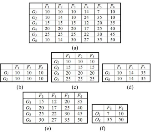
Based on the work of Madeira and Oliveira [21], the following four types of biclusters are generally assumed: (a) Bicluster with constant values, (b) Bicluster with constant values in rows or columns, (c) Bicluster with coherent values including additive or multiplicative models, (d) Bicluster with coherent evolutions. The first three types of biclusters deal with numerical values in the data matrix and try to find subsets of rows and columns with similar behaviors. Figure 2 shows the first three types of numerical biclusters that are hidden in a 6×6 data matrix. The bicluster with coherent evolutions aims to find coherent patterns regardless of the exact numeric values in the data matrix.
Fig. 2. (a) A 6×6 data matrix with hidden biclusters, (b) bicluster with constant values, (c) bicluster of constant rows, (d) bicluster of constant columns, (e) bicluster of additive model, where O3=O4−5=O5−10=O6−15 and F3=F4+3=F5-5=F6−20, (f) bicluster of multiplicative model, where O1=0.2×O6 and F5=0.7×F6.
3. Biclustering Algorithms
Many biclustering algorithms have been proposed. In this work, we classify biclustering algorithms into several categories depending on the bicluster model and the search strategy. We discuss the biclustering algorithms in each category briefly but put special emphasis on the geometric based biclustering recently proposed by our group.
Distance-based biclustering
Distance-based biclustering typically uses some distance-based variance metric to measure the quality of the biclusters, and performs an iterative search for the biclusters by minimizing the residual sum of squares cost. This class of biclustering algorithms is among the earliest biclustering methods proposed in the literature and is widely used in many applications [32-39]. In the “direct clustering” algorithm of Hartigan [32], the following sum of squares measure is used to evaluate the quality of each bicluster Bk = (Xk, Yk)
∈ ∈ − = k k k k Y j X i Y X ij k a a SSQ , 2 ) ( (1)where aX Yk k is the average value in the bicluster Bk. Biclusters with lower SSQ are considered to
and the solution is reached by minimizing the sum of SSQk. Obviously, the direct clustering
algorithm only search for constant biclusters.
In Cheng and Church’s δ-bicluster algorithm [33], biclustering is based on the minimization of a mean squared residue score
(
)
2 , 1 ( , ) ij iY Xj XY i X j Y H X Y a a a a X Y ∈ ∈ =
− − + (2)where aiY, aXj, aXY, are the row mean, column mean, and the mean in the submatrix B=(X, Y),
respectively. A bicluster is called a δ-bicluster if H(X, Y) ≤ δ for some δ > 0. To find the δ -bicluster, the score H is computed for each possible row/column addition or deletion, and the action that decreases H the most is applied. A bicluster is returned when H cannot be decreased or when H≤δ. After one δ-bicluster is identified, the elements in the corresponding submatrix are replaced by random numbers before finding the next δ-bicluster. The δ-biclusters are successively extracted from the raw data matrix one at a time until a pre-specified number of biclusters have been identified.
Following the work of Cheng and Church, different search strategies were proposed to better detect the δ-bicluster. In [40], Bryan et al. proposed a simulated annealing search technique and reported better performance on a variety of datasets. In [34, 35], Yang et al. proposed a probabilistic move-based algorithm called FLOC (FLexible Overlapped biClustering) that is able to discover multiple biclusters simultaneously. As a submatrix of a δ-bicluster is not necessarily a
δ-bicluster because of outliers, Wang et al. [36] proposed the δ-pCluster model to deal with the outlier problem by further requiring that any 2×2 submatrix in a δ-bicluster has a pScore≤δ for some δ > 0, where the pScore measures the difference between elements in the 2×2 submatrix.
Factorization-based biclustering
In contrast to biclustering algorithms that apply a greedy iterative search to find significant submatrices, factorization-based biclustering algorithm uses spectral decomposition technique to uncover “natural” substructures that are related to the main patterns of the data matrix [4, 41-43]. The spectral biclustering in [41] uses Singular value decomposition (SVD) and assumes that the data matrix has a checkerboard structure that can be identified in eigenvectors corresponding to characteristic patterns across samples or features. Using SVD, the data matrix DN×M can be
decomposed as D = UΛVT, where Λ is a diagonal matrix with decreasing non-negative entries, and U and V are N×min(N, M) and M×min(N, M) orthonormal column matrices. If the data matrix has a block diagonal structure (with all elements outside the blocks equal to zero), then each block can be associated with a bicluster. Specifically, if the data matrix is of the form
= r D D D D 0 0 0 0 0 0 2 1 (3)
where Di (i=1,…,r) are arbitrary matrices, then for each Di there will be a singular vector pair
(ui,vi) such that a nonzero component of ui corresponds to rows occupied by Di and a nonzero
component of vi corresponds to columns occupied by Di. In a less idealized case, when the
dominating values, the SVD is able to reveal the biclusters as dominating components in the singular vector pairs.
Nonnegative Matrix Factorization (NMF) has been recently introduced as a matrix factorization technique that produces a useful decomposition in the analysis of data [44]. NMF decomposes the data as a product of two matrices that are constrained by having nonnegative elements. The NMF is given by D≈WH, where D∈ℜp×n is a positive data matrix with p variables and n samples, W∈ℜp×q are the reduced q basis vectors or factors and H∈ℜq×n contains the coefficients of the linear combinations of the basis vectors needed to reconstruct the original data (also known as encoding vectors). As both the basis W and encoding vectors H are constrained to be non-negative, only additive combinations are possible. In [42, 43], Non-smooth Non-Negative Matrix Factorization algorithm (nsNMF), a variant of the NMF model, has been introduced to identify localized patterns in large datasets. In contrast to NMF, nsNMF produces sparse representation of the factors and encoding vectors by making use of non-smoothness constraints. The sparseness introduced by the algorithm produce more compact and localized feature representation of the data than the standard NMF.
In [45], a fuzzy biclustering technique is proposed. The technique is based on formulating the one-way clustering along the row and column dimension as a normalized graph cut problem. The graph cut problem is then solved by a spectral decomposition, followed by K-mean clustering of the eigenvectors. The biclustering of the row and column dimensions is achieved by a three-stage process. First, the original data matrix undergoes one-way clustering in the row dimension to obtain k clusters. Then, a new pattern matrix where each row is given by the average of the rows that belong to the same cluster in the original data matrix is computed. The new data matrix then undergoes the same one-way clustering in the column dimension to obtain k’ clusters. Finally, a table of fuzzy relation coefficients that relates each of the k row clusters to each of the k’ column clusters are computed. By computing the new data matrix using the result of the first stage clustering, the fuzzy biclustering algorithm achieves a biclustering of the original data matrix. Probabilistic based biclustering
The biclustering method in this category typically assumes a probabilistic model of biclusters and applies statistical parameter estimation techniques to search for the biclusters [46-49]. In the plaid model of Lazzeoni and Owen [48], the data matrix is viewed as consists of a series of additive layers, i.e. consists of biclusters or subsets of rows and columns. The model first includes a background layer which account for the global effects in the data matrix. Then, any subsequent layer represents additional effects corresponding to biclusters of objects and features that exhibit strong pattern not explained by the background layer. The generalized plaid model is given by
+ + = = K k ijk ik jk ij ij a 1 0 θ ρ κ ε μ (4)
where μ0 corresponds to the effect in the global background layer and θijk models the effect of
layer k. The effect θijk can be expressed as a combination of μk, αik, and βjk, where μk is the
background color in bicluster k, α and β are row and column specific additive constants in bicluster k. The parameter ρik (or κjk) equals 1 when object i (or attribute j) belongs to layer k,
and equals 0 otherwise. Any residual not modeled by the K layers is accounted for in the noise term εij. The biclustering process searches the layers in the data set one after another, using the EM algorithm to estimate the model parameters until the variance of expression levels within the current layer is smaller than a threshold. The plaid model provides a flexible framework for biclustering large, structured microarray dataset, as shown in [50].
In [47], Sheng et al. proposed a Bayesian technique for biclustering based on a simple frequency model for the expression pattern of a bicluster and on Gibbs sampling for parameter estimation. The data are discretized and every condition in a bicluster is modeled by a multinomial distribution, where the multinomial distributions for different conditions of a bicluster are assumed to be mutually independent. The Gibbs sampling sets the model in the Bayesian framework, and the Bernoulli posterior distribution is used during Gibbs sampling to find the biclusters. In [46], Gu and Liu proposed a fully generative models called Bayesian biclustering algorithm (BBC) for gene expression data. The data model in BBC is assumed to be
(
)
(
)
+ + + + − = = = K k K k ik jk ij jk ik ijk jk ik k ij e a 1 μ α β ε δ κ 1 1δ κ (5)where K is the total number of clusters (unknown), μk is the main effect of cluster k, and αik and βjk are the effects of sample i and feature j, respectively, in cluster k, εijkis the noise term for
cluster k, and eij models the data points that do not belong to any cluster. Here, δik=1 indicates that
sample i belongs to cluster k, and δik= 0 otherwise. Similarly, κjk=1 indicates that feature j is in cluster k, κjk= 0 otherwise. Gibbs sampling method is used for statistical inference in BBC.
Biclustering for coherent evolution
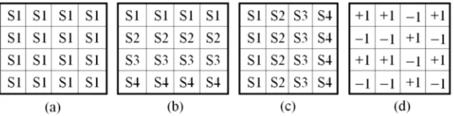
In bicluster analysis, the elements of a data matrix are usually of numeric values but they can also be transformed into symbols that reflect trends in the data. The symbols can be purely nominal, of a given order, or encode positive and negative changes relative to a normal value. Figure 3 shows examples of biclusters with coherent evolution. Several biclustering algorithms have been developed to find patterns with coherent evolutions.
Fig. 3. Types of biclusters with coherent evolution. Considering the entries of a data matrix as symbols, (a) an overall coherent evolution, (b) a coherent evolution on the rows, (c) a coherent evolution on the columns, (d) a coherent sign change across rows.
In [51], Ben-Dor et al. defined a bicluster as an order-preserving submatrix (OPSM). Specifically, a submatrix is order-preserving if there is a permutation of its columns under which the sequence of values in every row is strictly increasing. They define a complete bicluster model as the pair (Y,
π) where π=(y1, …, ys) is a linear ordering of the columns in Y. A row supports (Y, π) if the s corresponding values, ordered according to the permutation π, are monotonically increasing. Since an exhaustive algorithm that tries all possible models is not feasible, the algorithm grows partial models iteratively until they become complete models. Similarly, Liu and Wang define a bicluster as an OP-Cluster (Order Preserving Cluster) [52] which generalizes OPSM to discover biclusters with coherent evolutions on the columns.
In [53], Murali and Kasif introduced an algorithm that aims to find the largest xMOTIFs. An xMOTIF is defined as a bicluster with coherent evolutions on its rows. The data is first discretized into a set of symbols by using a list of statistically significant intervals for each row. The motifs are computed starting with a set of randomly chosen columns that act as seeds. For each column, an additional randomly chosen set A of columns is selected, called a discriminating set. The selected bicluster contains all the rows that have states equal to the seed column and in the columns contained in the discriminating set A. The motif is discarded if less than an α -fraction of the columns matches it. After all the seeds have been used to produce xMOTIFs, the largest xMOTIF (one with the largest number of rows) is returned.
Tanay et al. [54] introduced SAMBA (Statistical-Algorithmic Method for Bicluster Analysis) to detect the biclusters of coherent evolution. The data matrix is modeled as a bipartite graph. Discovering the most significant biclusters under the weighting schemes is equivalent to the selection of the heaviest subgraphs in the bipartite graph. SAMBA assumes that each aij can be
represented by two symbols S0 or S1, where S1 means change and S0 means no-change. As such, the model graph has an edge between a row and a column when the object is significantly changed with the feature. A large bicluster is one with a maximum number of rows whose symbol for aij is expected to be S1. In [29], Prelic et al. present a fast divide-and-conquer algorithm called
Bimax to detect the inclusion-maximal biclusters in the binary matrix E after a pre-discretization procedure. The Bimax algorithm is similar to SAMBA. The idea behind the Bimax algorithm is to partition E into three submatrices, one of which contains only 0-cells and therefore can be disregarded in the results. The algorithm is then recursively applied to the remaining two submatrices U and V. The recursion ends if the current matrix represents a bicluster, i.e. contains only 1s. If U and V do not share any rows and columns of E, the two matrices can be processed independently from each other. However, if U and V have a set X of rows in common, special care is necessary to only generate those biclusters in V that share at least one common column with X. In [55], Uitert et al. propose BicBin (Biclustering Binary data) to find a contiguous block for a large, binary, and sparse genomic data matrix, such as transcription factor binding site, insertional mutagenesis and gene expression. Assuming that each element in D is the outcome of a Bernoulli trial, a probability based score function is derived in BicBin to evaluate a submatrix. Geometric-based biclustering
Based on a spatial interpretation of biclusters, we have recently proposed a geometric-based biclustering framework [28, 56, 57]. The geometric viewpoint makes this class of algorithms radically different from most existing algorithms which are typically based on optimizing certain heuristically defined merit functions. The geometric viewpoint provides a unified mathematical formulation for the simultaneous detection of different types of linear biclusters (i.e. constant, additive, multiplicative, and mixed additive and multiplicative biclusters) and allows biclustering to be done with a generic plane detection algorithm.
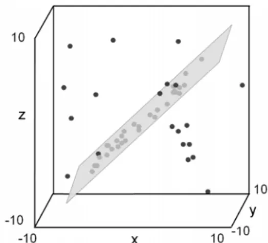
The theoretical basis of geometric-based biclustering is as below. If we consider that the set of columns Y in B = (X, Y) spans a ||Y||-dimensional space, then the data vector in every row of B corresponds to a point in this space. Thus, from a geometric viewpoint the different biclusters can be considered as different linear geometric patterns in the high dimensional data space. For example, given a matrix DN×3, a bicluster is represented by a plane in a 3D space as shown in Fig. 4, where the N 3D samples are represented by N points. Obviously, a plane can be detected within the 3D data space which provides clues about the hidden bicluster in D. In geometric based biclustering, the problem of identification of coherent sub-matrices within a data matrix is formulated as the detection of linear geometric patterns (lines, planes, or hyperplanes) in a multidimensional data space [28].
Fig. 4 A plane formed by points in a bicluster in the three-dimensional data space. The grey dots are data located on the plane.
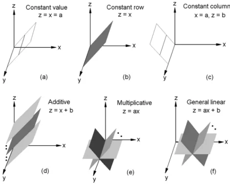
Figure 5 shows the six bicluster patterns that form linear geometric patterns in the data space: (a) constant values, (b) constant rows, (c) constant columns, (d) additive coherent values, where each row or column is obtained by adding a constant to another row or column, (e) multiplicative coherent values, where each row or column is obtained by multiplying another row or column by a constant value, and (f) linear coherent values, where each column is obtained by multiplying another column by a constant value and then adding a constant. Of these six patterns, the linear coherent model of (f) subsumes all previous five patterns. These bicluster patterns correspond to the commonly used bicluster patterns discussed earlier. Although the six patterns in Fig. 5 appear to be substantially different from each other, if we treat each column as a variable in the 4D space [x, y, z, w] and each row as a point in the 4D space, the six patterns in Fig. 5 (a) to (f) would correspond to the following six geometric structures: (a) a bicluster at a single point with coordinate [x, y, z, w] = [1.2, 1.2, 1.2, 1.2], (b) a bicluster defined by the lines x = y = z = w, (c) a bicluster at a single point with coordinate [x, y, z, w] = [1.2, 2.0, 1.5, 3.0], (d) a bicluster defined by the lines x = y – 1 = z + 1 = w – 2, (e) a bicluster defined by the lines x = 0.5y = 2z = 2w/3, and (f) a bicluster defined by the lines x = 0.5(y – 0.1) = 2(z – 0.1) = 2(w – 0.2)/3. Each row in a bicluster is a point lying on one of these points or lines.
Fig. 5 Examples of different bicluster patterns: (a) constant values, (b) constant rows, (c) constant columns, (d) additive coherent values, (e) multiplicative coherent values, and (f) linear coherent values.
When a pattern is embedded in a larger data matrix with extra measurements, i.e., a bicluster that covers only part of the measurements in the data, the points or lines defined by the bicluster would sweep out a hyperplane in a high dimensional data space. To illustrate this in a 3D space, if we denote the three measurements as x, y and z respectively, and assume a bicluster covers x and z only, we can generate 3D geometric views for different patterns as shown in Fig. 6. When the dimensions of the data space are more than three, visualizing them becomes difficult, but the geometric structures are still similar.
Fig. 6 Different geometries (lines or planes) in the 3D data space for corresponding bicluster patterns. (a) A bicluster with constant values: represented by one of the lines that are parallel to the y-axis and lie in the plane x = z (the T-plane), (b) a bicluster with constant rows: represented by the T-plane, (c) a bicluster with constant columns: represented by one of the lines parallel to the y-axis, (d) a bicluster with additive coherent values: represented by one of the planes parallel to the T-plane, (e) a bicluster with multiplicative coherent values: represented by one of the planes that include the y-axis , and (f) a bicluster with linear coherent values: represented by one of the planes that are parallel to the y-axis.
The geometric interpretation of bicluster patterns has the important implication in that it unifies the commonly used bicluster patterns into a single linear class and allows a unified treatment in detecting these linear biclusters simultaneously. This is in contrast to most existing biclustering algorithms where the cost function implicitly imposes a constraint on the type of bicluster patterns that could be discovered. In theory, any algorithm for detecting linear geometric patterns
can be employed in the geometric biclustering framework. We have employed well-known image processing methods for geometric biclustering, such as the Hough transform (HT) and relaxation labeling. The HT is a well-known technique to detect lines and planes in multidimensional data space. Statistical properties of the HT, such as robustness, consistency and convergence, as well as their ability to identify geometric patterns in noisy data, make them highly attractive for bicluster analysis of noisy microarray data [58, 59].
The HT is a methodology that detects lines and curves in images through a voting process in two dimensional parameter spaces. Given a set of points {xi = (x1i, x2i) ∈R2: i=1,…, n}, the objective
is to infer the parameters (a1, a2) of the line x2i= a1x1i+a2 which fit the data {xi} optimally. The
key to the HT algorithm is to view each point as generating a line comprising all pairs (a1 and a2) that are consistent with this point. Thus the collinearity in the original set of points will manifest itself in a common intersection of lines in the Hough domain. To obtain the intersecting point of lines, the Hough domain is first quantized into cells, and each cell maintains a count of the number of intersecting lines. The cell with the largest number of counts is the obvious estimator of the parameters of the original line. In practice, polar coordinates are used to describe the line in the Hessian normal form instead of the direct parameter space. This allows for the detection of vertical lines (θ=π/2) in the data set, and moreover guarantees an isotropic error in contrast to direct parameterization.
In [28], we used the Fast Hough Transform (FHT) [60] as our plane detection algorithm since it gives considerable speedup and requires less storage requirement than the conventional HT. The FHT has very simple and efficient high-dimensional extension and it uses a coarse-to-fine mechanism which provides very good noise resistibility. In [28], we applied the FHT to the entire data matrix using an efficient K-tree data structure. In the algorithm, we represent the parameter space as a nested hierarchical hypercube where the FHT recursively divides the parameter space into hypercubes from low to high resolutions, and the subsequent vote counting in parameter space is done only in hypercubes with votes exceeding a selected threshold. A hypercube with acceptable resolution and with votes exceeding a selected threshold indicate a detected hyperplane in the observed data.
With the emergence of microarray data compendiums such as ArrayExpress and GEO, microarray data sets comprising thousands of genes and hundreds of conditions are common sources for module discoveries and pathway discoveries in systems biology. Biclustering algorithms are obliged to be able to deal with the huge and ever-growing microarray datasets. To handle very large gene expression data matrix, a divide and stitch strategy was proposed in [61]. The basic idea is to divide the data matrix into several non-overlapping blocks where each block includes all genes but different conditions. The geometric biclustering algorithm is then applied to each block. Finally, for a detected bicluster in a block, a check is performed to see whether conditions from other blocks can be incorporated into it as well as deleting any duplicated biclusters.
In [56], a sub-dimension based geometrical biclustering algorithm (GBC) was proposed which only performs the HT in every 2-D feature space, called the column-pair space. The strategy is based on finding the simultaneous equations of the geometric structure in column-pair space. For example, instead of finding a pattern satisfying x1= x2= x3= x4 in a 4-D space, GBC detects
patterns satisfying x1= x2, x2= x3, x3= x4 in three 2-D spaces and then combines them. Therefore,
the GBC algorithm starts from all n(n−1)/2 unique column-pairs of the data matrix. Then the sub-biclusters in column-pair spaces are combined to form a complete bicluster according to the criterion that any two sub-biclusters with at least one common feature (sample) can be combined into a new one where the common samples (features) are retained. The strategy reduces the computational complexity considerably and makes it possible to analyze large-scale microarray data.
using the relaxation labeling framework for the sub-bicluster merging based on their geometric distance. In the relaxation procedure, the contextual information is employed to classify a set of interdependent samples by allowing interactions among the possible classifications of related samples. The relaxation framework makes the GBC less sensitive to noise and allows the discovery of larger biclusters.
4. Bicluster Validation
Validating the detected biclusters is an important but challenging problem due to the different criteria used and the different goals in biclustering. In this section, we discuss several common validation strategies for biclustering results including index based validation, validation using domain knowledge, and statistical testing.
Index based validation
Traditional clustering is based on some measure of distance and many indexes, such as the Silhouette method, Dunn index, Davies–Bouldin index, and the C-index, are employed to assess the clusters’ quality of compactness, connectedness, variance and robustness [61]. However, the variety of coherent patterns in biclustering makes bicluster validation difficult. If ground truth is available, the biclustering results can be assessed by measuring how well the discovered biclusters match the true biclusters. To compare two biclusters A =(X1, Y1) and B=(X2, Y2), the Jaccard index can be used,
| | | | | | | | ) , ( B A B A B A B A JacInd ∩ − + ∩ = (6)
where |•| denotes the number of elements [62].
In [29, 63, 64], the original Jaccard index is improved by using match score. Let B1and B2be the set of true biclusters in the data matrix and the set of detected biclusters, respectively. The match score of B1with respect to B2is given by
( ) ( ) 2 2 2 1 1 1 1 2 1 2 1 2 , , 1 1 2 1 2 1 ( , ) max XY X Y B X Y B X X Y Y S B B B ∈ ∈ X X Y Y ∩ + ∩ = ∪ + ∪
(7) When all the true biclusters are detected, SXY(B1,B2) = 1. However, such validation method doesnot consider the false biclusters Bf which could account for a large number of the detected
biclusters B2. An algorithm that returns only the true biclusters would give the same matching score as another algorithm that returns the true biclusters as well as some false biclusters. In our comparative study, we take the false biclusters into account by dividing B2 into two parts: Bf =
(Xf,Yf) that shares no common elements with the true biclusters and Br= (Xr,Yr) that shares some
common elements with the true biclusters. Our modified match score is then given by
( ) ( 1 1) 1 1 1 1 2 , , 1 1 1 1 ( , ) max r r r r r XY X Y B X Y B r f r f X X Y Y S B B B ∈ ∈ X X X Y Y X ∩ + ∩ = ∪ ∪ + ∪ ∪
(8)In simulation studies, the matching scores provide an intuitive measure to assess the quality of the resulting biclusters in comparison to the true biclusters. If Bopt denotes the set of true biclusters
and B denotes the set of biclusters produced by a biclustering method, then SXY(Bopt, B) reflects to
When no ground truth is available, the quality of a bicluster can be assessed by how compact the bicluster is. One such measure is the mean squared residual error (MSR) which measures the deviation of values in a bicluster from the mean value of the bicluster [33, 34, 65]. However, MSR is only appropriate for constant value biclusters. Instead of measuring the residual error, the coherent of a bicluster can be measured by the correlation values between rows or columns. Teng and Chan [66] proposed to use the average correlation value (ACV) to assess the quality of a bicluster. The ACV of a bicluster is defined by
[ ]
0,1 , max ) ( 2 2 ⊆ − − − − =
∈ ∈
∈ ∈ Y Y Y r X X X r B ACV i X j X ij kY lY kl (9)where rij is the weighted correlation between the rows of B and rkl is the weighted correlation
between the columns of B. The weighted correlation coefficient between samples a and b is given by
(
)
(
)
(
(
)
)
− − − = i i i i i i i i i i i i i i i i i i i i i i b m b m a m a m b m a m b a m r 2 2 2 2 (10)where m is the feature weight vector.
If the quality criterion for a bicluster is how well the rows or columns are related by a monotonic function, then a quality index based on the Spearman’s rank correlation coefficient can be used. In [67], the average Spearman’s rho (ASR) is employed as the evaluation function
[ ]
1,1 , max 2 ) ( 2 2 ∈ − − − − − ∗ =
∈ ∈
∈ ∈ Y Y Y X X X B ASR i X j X ρij k Y l Yρkl (11)where ρij and ρkl is the Spearman’s rank correlation associated with the rows and columns in B
respectively.
In [30], Lee et al. proposed an index Γ that measures the extent that similar objects are grouped together. Let P=(pij) be the proximity matrix of objects where pij denotes the distance between
two objects Oi and Oj, and let C=(cij) be the membership matrix with cij =1(1+kij) where kij is
the number of biclusters that Oi and Oj simultaneously belong to. Then the Hubert statistic of
objects can be defined as
(
)
(
p c)(
)
n i n i j ij p ij c O c p n n σ σ μ μ
− = =+ − − − = Γ 1 1 1 1 2 (12)where µp (µc) and σp (σc) are the mean and standard deviation of P (C) respectively. The statistic
of features ΓF can be formulated similarly. Then, the Γ index is defined by combining the two
statistics as follows m n m n O F + Γ + Γ = Γ (13)
Since the numerator increases as similar objects or features are grouped together, a bicluster solution with large Γis preferred.
Validation using domain knowledge
One way for evaluating bicluster algorithms is by using prior knowledge as some form of a gold standard to compare to the biclusters. With a known classification of samples or features, the p -values can be computed for the validation [25]. For example, suppose we know that the M samples are partitioned into k classes, C1, …. , Ck. Let B be a bicluster with b objects. Assuming
its most abundant class is Ci, and r objects in B belong to Ci. Then B is enriched in Ci if it has a
small p-value, which is calculated as
− − = b M r b C M r C B) i i ( value -p (14)
The p-value measures the probability of including objects of a given category, i.e. Ci, in a
bicluster B by pure chance. Thus, the overrepresented bicluster is a bicluster of objects which is very unlikely to be obtained randomly. One should note that high quality biclusters can also identify phenomena that are not covered by the given classification. Nevertheless, a large fraction of the biclusters is expected to conform to the known classification. If the true biclusters are known in simulation, some traditional statistic, such as sensitivity and specificity, can also be used for the comparison of biclustering results [46].
In the biclustering of gene expression data, we sometime have prior knowledge about the biological conditions. Due to known biological conditions, the p-values can be used to assess the statistical significance of biclusters. To date, Gene Ontology (GO), metabolic pathway maps (MPM), and protein-protein interaction networks (PPI) have been used to determine the biological functional relevance of genes and gene products in a bicluster. Using the known gene annotation structure in GO, MPM and PPI, the p-values of genes associated with the biclusters can be computed for biological validation [25, 28, 29, 50, 63].
Validation through statistical test
The statistical significance of a biclustering result can be evaluated by comparing the result to a random partitioning of the data matrix. The details of randomization may be critical to the integrity of such a test and needs to be taken into consideration. For example, in [47], the data are first randomized according to a uniformly random graph model.
5. Bicluster Visualization
Visualization of biclustering results is difficult due to the noncontiguous and overlapping indexing in both the row and column. The most popular visualization technique to represent a single bicluster is the heatmap technique [20, 28]. A heatmap is a rectangular grid composed of pixels each of which corresponds to a data value. The different gray/color scales correspond to the different data values. Usually, the brighter the color is, the larger the value. This way, if the rows and/or columns of the dataset are re-ordered appropriately, the bicluster pattern becomes obvious visually. Heatmaps usually suffice for the purpose of inspecting a single bicluster. Figure 7(a) is a heatmap of a matrix and Fig. 7(b) is the visualization of a bicluster of constant rows by reordering the indexes of rows and columns appropriately.
Parallel coordinates (PC) have also been used to represent biclusters, but they are less widely used than heatmaps [25, 68]. The PC technique is a powerful method for visualizing and analyzing high-dimensional data under a two-dimensional setting. In the PC technique, each feature is represented as a vertical axis, and the N-dimensional axis is arranged in parallel to each other. By giving up the orthogonal representation, the number of dimensions that can be
visualized is not restricted to only two. Studies have found that geometric structure can still be preserved by the PC plot despite the fact that the orthogonal property is destroyed [25]. In the visualization of biclusters, the data sample i is an N-dimensional point pi=(ai1, ai2, ...aiN) where aij
is the value of the feature j insample i and the N features are visualized as vertical axes. The work in [25] shows that the PC technique can not only be used to visualize the biclustering results but can also be used to discover biclusters.
The dendrogram is a commonly used tool to present hierarchical clustering results where the detected structures can be further divided in substructures recursively [19]. Usually, clustering is only applied to either rows or columns. Due to two dimensional clustering, biclustering results are displayed with two dendrograms by rearranging the indexes along two dimensions (see Fig. 7(c)).
Fig. 7. Visualization techniques of biclustering patterns: (a) The heatmap of a data matrix; (b) a heatmap showing one hidden bicluster pattern embedded in the data matrix by permuting the rows and columns appropriately; (c) two-way traditional dendrogram.
6. Comparative Study of Different Biclustering Algorithms
In order to compare the performance of biclustering algorithms, we tested ten biclustering algorithms on both artificial and biological datasets. The well known conventional K-means clustering is also compared. The GBC algorithm is implemented by us. The BBC software can be downloaded from http://www.people.fas.harvard.edu/~junliu/BBC/. FLOC is implemented in the R package called ‘biare’ while spectral biclustering and plaid model biclustering are included in the R package called ‘biclust’. The CTWC and NMF biclustering algorithms are from http://ctwc.weizmann.ac.il/process.aspx and http://bionmf.cnb.csic.es/, respectively. SAMBA is from Expander, whereas Bimax, and K-means are from BicAT, and they can be downloaded from http://acgt.cs.tau.ac.il/expander/ and http://www.tik.ee.ethz.ch/sop/bicat/, respectively. The BiHEA biclustering algorithm is from BAT and can be found on
http://lidecc.cs.uns.edu.ar/index.php?option=com_content&view=article&id=44&Itemid=32. Experiments with Artificial Dataset
In the first experiment, we test the performance of the algorithms for noisy data. We embed 10 non-overlapping constant and additive patterns of 20 columns and 20 rows with Gaussian noise of variance ranging from 0.1 to 0.5 into a 500 by 200 matrix. In the second experiment, we test the effectiveness of the algorithms for resolving overlapped patterns. We embed 10 overlapped additive patterns of 20 columns and 20 rows with Gaussian noise of variance ranging from 0.1 to 0.5 randomly into a 500 by 200 matrix with overlapping degrees from 2 to 10, representing the number of rows or columns that overlap. The background data of both datasets are sampled from a uniform distribution U(−20,20). The modified match score of (8) is used for validation.
Figure 8 illustrates the performance of the biclustering algorithms. Figures 8(a) and 8(b) show that spectral biclustering, CTWC, and plaid model biclustering perform as bad as the conventional clustering methods such as K-means in detecting constant and additive patterns in the data matrix. The matching scores for these methods are lower than 20% even for low noise level. The NMF, GBC and SAMBA algorithms show a far better performance (>80%) than other biclustering algorithms in constant pattern detection while the GBC and Bimax algorithms show a better performance (>80%) in detecting additive patterns than the other algorithms for all noise level. Figure 8(c) shows the performance of biclustering algorithms for varying overlapping degree of bicluster pattern. From the matching score curves, we can see that GBC, Bimax and SAMBA show good performance (>80%) when the overlapping degree is low, but the performance of Bimax and SAMBA deteriorates with increasing degree of overlap.
(a)
(c)
Fig. 8 Matching score curve: (a) The performance of different algorithms for constant bicluster patterns with noise variance from 0 to 0.5. (b) The performance of different algorithms for additive bicluster patterns with noise variance from 0 to 0.5. (c) The performance of different algorithms for additive patterns with overlapping degree from 2 to 10.
Experiments with Biological dataset
We make use of microarray data called ‘BicatYeast’ composed of 70 columns and 420 rows, which can be obtained from R package ’biclust’. After biclustering the microarray gene expression data, we study whether the set of genes in the detected bicluster show significant enrichment with respect to GO annotation using a web tool called DAVID (http://david.abcc.ncifcrf.gov/). The p-value of genes are calculated and adjusted for validation. Figure 9 illustrates the enrichment of the gene set in the first five biggest biclusters discovered by the algorithms. The x-axis shows the biclustering algorithms with different p-values while the y-axis is the percentage of genes in the biclusters annotated by GO. The result shows that the genes in the biclusters detected by GBC and spectral biclustering methods are more highly enriched with GO biological process categories than that detected by other biclustering/clustering algorithms. It is interesting to note that even though spectral biclustering performs badly in the artificial datasets, its performance is much better on the biological dataset. The poor result for artificial datasets could be due to the checkerboard structure not been present in the artificial datasets. Finally, almost all biclustering algorithms other than plaid model biclustering show better result than K-means clustering in the biological dataset. The result demonstrated that traditional clustering techniques have difficulty extracting highly localized expression patterns.
Fig.9 GO biological process enrichment analysis results for the biclustering algorithms.
7. Biclustering Applications
As an unsupervised technique, biclustering can be applied to any data matrix to identify the subsets of rows and columns with certain coherent patterns. The output of a biclustering algorithm is a collection of significant local coherent patterns in the data. Such patterns may be useful in diverse applications. Apart from the main application in gene expression data analysis, biclustering is also employed in other biological applications, such as sequence alignment, transcription factor binding, and insertion mutagenesis. In addition, many other application domains such as text mining and financial market analysis have also being investigated.
Biological applications
The majority of the recent applications of biclustering are in biological data analysis, especially gene expression data [21-25, 27-29, 31, 33, 35, 37, 40-43, 46-48, 50-57, 63-70]. As a revolutionary new tool, DNA microarray technology is a high-throughput platform that can provide expression profiling of thousands of genes in different biological conditions, thereby enabling the rapid and quantitative analysis of gene expression patterns on a global scale [19]. Many DNA microarray studies are related to the study of cancer [8-10, 12, 13, 15-17]. In DNA gene expression data analysis, a typical objective is to discover groups of genes that share similar transcriptional characteristics in gene function, tissue classification, and motif identification. Biclustering is able to capture co-regulation expression patterns that involve subsets of genes and subsets of conditions and has been used for the inference of global regulatory networks [69]. Biclustering is particularly useful in gene expression data analysis, where an interesting cellular process is active only in a subset of conditions or a single gene may participate in multiple pathways that may not be co-active under all conditions. For gene expression data, it is expected that only a small subset (a few tens) of genes in a dataset is involved in a particular process of interest (such as cancer), while the vast majority (thousands) of the genes play no role in the process. Similarly, the genes that belong to the relevant subset may have highly correlated expression only over those columns (i.e. the samples in gene expression data matrix) in which the process of interest actually takes place. Including irrelevant genes or samples into the clustering will mask out these correlations.
Apart from DNA microarray data, biclustering is used in a number of other molecular biology applications. In [71], Wang et al. applied biclustering to multiple sequence alignment (MSA) of
RNA data. A challenge in MSA is that the alignment of sequences is often intended to reveal groups of conserved functional subsequences. Simultaneously, the grouping of the sequences can impact on the alignment; precisely the kind of dual situation biclustering is intended to address. In [72], Lottaz et al. applied biclustering to discover clinically relevant patient subgroups by combining expression data with functional annotation data. In [55], Uitert et al. developed the BicBin algorithm for binary genomic data and applied the algorithm to transcription factor binding and insertion mutagenesis. In [52], Liu and Wang applied biclustering to a drug activity dataset to associate common properties of chemical compounds with common groups of their descriptors.
Medical applications
In [73], biclustering is utilized to analyze scalp EEG data obtained from epileptic patients undergoing treatment with a vagus nerve stimulator (VNS) implant. The device consists of an electric stimulator implanted subcutaneously in the chest and connected, via subcutaneous electrical wires, to the left cervical vagus nerve. The VNS is programmed to deliver electrical stimulation at a set intensity, duration, pulse width, and frequency. The study examines the EEG effects of VNS stimulation with the aim to develop a physiologic marker for optimal VNS parameters. Each EEG channel is represented as a data feature and samples taken from within and outside the stimulation periods are analyzed. The study has shown that it is possible to distinguish VNS stimulation from VNS deactivation epochs using scalp-EEG recordings.
In [74], biclustering is applied to the computer-aided diagnosis of digital mammography images. With the rows representing the set of images and columns representing the set of features, biclustering can find a subset of images participating in a common pathology of interest while defining a subset of features that best describe this pathology. The study analyze a data matrix consists of 213 images and 224 features using K-means clustering and SAMBA biclustering algorithms.
Text mining
Biclustering can be used successfully to identify subgroups of documents with similar properties relative to subgroups of attributes. The text is represented by a data matrix D = (aij)M×N, where
each row corresponds to a document, each column to a word (or term), and the value of aijis a
certain weight of word i in the document j. In the simplest case, this weight can be, for example, the number of times the word i appears in text j. Text mining techniques are of high importance for text indexing, document organization, text filtering, web search, etc. Generally, one-way clustering can be used to classify the text data such as word and document data. Biclustering of text data allows not only the clustering of documents and words simultaneously, but also discovers important relations between document and word classes. Successful biclustering approaches for text mining were developed based on a spectral approach or on an information theoretic technique [75-77].
Multimedia data processing and retrieval
In [78], a biclustering based real-time rendering algorithm to render all-frequency radiance transfer at both the macro- and meso-scale is proposed. For a given local incident direction dj at
vertex p, the transfer matrix element (Tp)jk represents the contribution of the global incident
direction dk. In other words, the element indicates how much of the global incident radiance at dk
would reach the local incident radiance direction dj. As the large transfer matrix needs to be
stored and manipulated, biclustering is used to compress the transfer matrix by exploiting the sub-matrices having constant column entries in the transfer matrix. By decomposing the transfer
matrix into bicluster submatrices, an efficient bicluster representation can be obtained. The algorithm is able to reduce storage and computational complexity down to 5%-30%, enabling real-time rendering.
In [79], biclustering was applied to video document retrieval. Video document consists of many media modalities such as audio track, textual tags and visual frames, and the video contents and associated semantics could have no direct correlation with low-level features. Noise in the feature space also result in extra complexity in the measurement of document relevance and degrade retrieval performance. Biclustering was used to select the feature subspace that best discriminate the different class of content. In [80], biclustering was applied to content-based image retrieval by combining information from visual data and text annotation. The biclustering is used to uncover the semantic connection between the image features and the text. It was demonstrated that the biclustering of image segments and annotation words significantly improved the performance of the image retrieval system.
Other applications
Biclustering can be used in collaborative filtering to find subgroups of customers with similar attitudes or behavior towards a subset of products, with applications in target marketing or recommendation system. In such applications, the value aij in the data matrix is whether
customer i expresses in some way the investigated attitude or behavior j. A number of papers consider collaborative filtering of movies, where the data values are either binary (i.e., showing whether a certain customer watched a certain movie or not) or express the rate at which a customer is assigned to a movie [36, 81, 82]. Biclustering has been applied to the study of social annotations to discover associations among a group of users and resources, and identifying user communities [83]. Social annotation allows web users with explicit or implicit social interactions to annotate web resources or objects such as bookmarks and photographs without a predefined formal ontology, in order to retrieve and share information more efficiently. In [45], a fuzzy biclustering algorithm is proposed to identify groups of related web users and web pages. The results would be useful for applications such as user profiling for web personalization systems and recommendation engines, improved web information retrieval, as well as in the design of more efficient caching and prefetching policies. In [48], biclustering is applied to nutritional data where each sample is associated with a certain food and each feature is an attribute of the food. The goal was to form clusters of foods with respect to a similar subset of attributes. Other applications of biclustering include dimensionality reduction of databases via automatic subspace clustering of high dimensional data [80], analyzing the electoral data to identify sub-groups of countries with similar electoral preferences/political attitude toward certain issues [32], and grouping a set of foreign exchange rates together based on the fact that they have a certain type of defined correlation in a certain set of time points [84].
8. Conclusions
Biclustering, which aims to detect subsets of objects and subsets of attributes that exhibit certain coherent pattern, has found many uses in many real world applications. In this paper, we present a survey of the biclustering algorithms, their performance evaluation, and applications. We discuss the different bicluster patterns that are commonly used. Although there is a lack of a general definition of homogenous patterns in biclustering, we show that the recent geometric view of biclustering provides a useful framework that unites all linear biclusters. We categorize biclustering algorithms into several categories based on the merit function used, the algorithmic framework, and the bicluster patterns to be detected. With the many biclustering algorithms available today, validation of the biclustering results is an important issue. We discuss three
strategies that can be used to validate biclustering results: index based validation, validation using domain knowledge, and validation through statistical test. We discuss how the biclustering results can be visualized effectively. We present evaluation results on ten well-known biclustering algorithms using both artificial and real gene expression datasets. Finally, we describe some of the diverse applications where biclustering has been found to be a useful analysis tool. We believe that the ability to extract local patterns and behaviors in biclusters should find a wide range of applications in many problems where simultaneous clustering of objects and features are important.
Conflict of Interest
The authors declare no conflict of interest in the publication of this manuscript. Acknowledgements
This work is supported by the Hong Kong Research Grant Council (Project CityU 123809), the Australian Research Council's Discovery Projects funding scheme (Project No. DP1097059), and the National Natural Science Funds of China (Project No. 31100958).
REFERENCES
[1] Anderberg MR. Cluster analysis for applications. New York : Academic Press, 1973.
[2] Clatworthy J, Buick D, Hankins M, Weinman J, Horne R. The use and reporting of cluster analysis in health psychology: A review. British Journal of Health Psychology 2005; 10: 329-358.
[3] Vogt W, Nagel D. Cluster analysis in diagnosis. Clinical Chemistry 1992; 38:182-198.
[4] Filippone M, Camastra F, Masulli F, Rovetta S. A survey of kernel and spectral methods for clustering. Pattern Recognition 2008; 41: 176-190.
[5] Hruschka E, Campello R, Freitas A, Carvalho A. A Survey of Evolutionary Algorithm for Clustering. IEEE Trans. Syst., Man, Cybern. C, Appl. Rev. 2009; 39(2): 133-155.
[6] Wu S, Liew AWC, Yan H. Cluster Analysis of Gene Expression Data Based on Self-Splitting and Merging Competitive Learning. IEEE Trans. Information Technology in Biomedicine 2004; 8(1): 5-15. [7] Borland J, Hirschberg J, Lye J. Data Reduction of Discrete Responses: An Application of Cluster
Analysis. Applied Economics Letters, Taylor and Francis Journals 2001; 8(3):149-53.
[8] Alizadeh AA, Eisen MB, Davis RE et al. Distinct Types of Diffuse Large B-Cell Lymphoma Identified by Gene Expression Profiling. Nature 2000; 403: 503-511.
[9] Alon U, Barkai N, Notterman DA et al. Broad Patterns of Gene Expression Revealed by Clustering of Tumor and Normal Colon Tissues Probed by Oligonucleotide Arrays. Natural Academy of Sciences 1999; 96(12): 6745-6750.
[10] Armstrong SA, Staunton JE, Silverman LB et al. Mll Translocations Specify a Distinct Gene Expression Profile that Distinguishes a Unique Leukemia. Nature Genetics 2002;. 30: 41-47.
[11] Cho RJ, Campbell MJ, Winzeler EA et al. A Genome-Wide Transcriptional Analysis of the Mitotic Cell Cycle. Molecular Cell 1998; 2: 65-73.
[12] Gasch AP, Huang M, Metzner S, Botstein D, Elledge SJ, Brown PO. Genomic Expression Responses to DNA-Damaging Agents and the Regulatory Role of the Yeast ATR Homolog mec1p. Molecular Biology of the Cell 2001; 12:2987-3003.
[13] Golub TR, Slonim DK, Tamayo P et al. Molecular Classification of Cancer: Class Discovery and Class Prediction by Gene Expression Monitoring. Science 1999; 286:531-537.
[14] Hughes TR, Marton MJ, Jones AR et al. Functional Discovery via a Compendium of Expression Profiles. Cell 2000; 102:109-126.
[15] Iyer VR, Eisen MB, Ross DT et al. The Transcriptional Program in the Response of Human Fibroblasts to Serum. Science 1999; 283:83-87.
[16] Klein U, Tu Y, Stolovitzky GA et al., Gene Expression Profiling of B Cell Chronic Lymphocytic Leukemia Reveals a Homogeneous Phenotype Related to Memory B Cells. J. Experimental Medicine 2001; 194:1625-1638.
England J. Medicine 2000; 344(8): 539-548.
[18] Spellman PT, Sherlock G, Zhang MQ et al. Comprehensive Identification of Cell Cycle-Regulated Genes of the Yeast Saccharomyces Cerevisiae by Microarray Hybridization. Molecular Biology of the Cell 1998; 9:3273-3297.
[19] Eisen MB, Spellman PT, Brown PO, Botstein D. Cluster analysis and display of genome-wide expression patterns. Proc. Natl. Acad. Sci. 1998; 95:14863–14868.
[20] Busygin S, Prokopyev O, Pardalos PM. Biclustering in Data Mining. Computers & Operation Research 2008; 35: 2964-2987.
[21] Madeira SC, Oliveira AL. Biclustering Algorithms for Biological Data Analysis: a Survey. IEEE/ACM Trans. Computational Biology & Bioinformatics 2004; 1(1):24-45.
[22] Bleuler S, Prelić A, Zitzler E. An EA framework for biclustering of gene expression data. Proceedings of Congress on Evolutionary Computation 2004; pp. 166-173.
[23] Divina F, Ruiz JA. Biclustering of expression data with evolutionary computation. IEEE Trans. Knowledge & Data Engineering 2006;18:590-602.
[24] Mitra S, Banka H. Multi-objective evolutionary biclustering of gene expression data. Pattern Recognition 2006; 39(12):2464-2477.
[25] Cheng KO, Law NF, Siu WC, Liew AWC. Identification of Coherent Patterns in Gene Expression Data Using an Efficient Biclustering Algorithm and Parallel Coordinate Visualization. BMC Bioinformatics 2008; 9: 210.
[26] Grothaus GA, Mufti A, Murali TM. Automatic layout and visualization of biclusters. Algorithms for Molecular Biology 2006; 1:15.
[27] Santamaria R, Theron R, Quintales L. A Visual Analysis Analytics Approach for Understanding Biclusters Results from Microarray Data. BMC Bioinformatics 2008; 9:247.
[28] Gan X, Liew AWC, Yan H. Discovering Biclusters in Gene Expression Data Based on High-dimensional Linear Geometries. BMC Bioinformatics 2008; 9:209.
[29] Prelic A, Bleuler S, Zimmermann P et al. A Systematic Comparison and Evaluation of Biclustering Methods for Gene Expression Data. Bioinformatics 2006; 22: 1122–1129.
[30] Lee Y, Lee JH, Jun CH. Validation Measures of Bicluster Solutions. Industrial Engineering & Management Systems 2009; 8:101-108.
[31] Tanay A, Sharan R, Shamir R. Biclustering Algorithms: A Survey. Handbook of Computational Molecular Biology, Edited by S. Aluru, Chapman & Hall/CRC, Computer and Information Science Series, 2005.
[32] Hartigan JA. Direct Clustering of a Data Matrix. J. Am. Statistical Assoc. 1972; 67(337):123-129. [33] Cheng Y, Church GM. Biclustering of Expression Data. Proc. Eighth Int’l Conf. Intelligent Systems
for Molecular Biology (ISMB ’00) 2000; pp. 93-103.
[34] Yang J, Wang W, Wang H, Yu P. δ-Clusters: Capturing Subspace Correlation in a Large Data Set. Proc. 18th IEEE Int’l Conf. Data Eng. 2002, pp. 517-528.
[35] Yang J, Wang W, Wang H, Yu P. Enhanced Biclustering on Expression Data. Proc. Third IEEE Conf. Bioinformatics and Bioeng. 2003, pp. 321-327.
[36] Wang H, Wang W, Yang J, Yu P. Clustering by Pattern Similarity in Large Data Sets. Proc. 2002 ACM SIGMOD Int’l Conf. Management of Data 2002, pp. 394-405.
[37] Getz G, Levine E, Domany E. Coupled Two-Way Clustering Analysis of Gene Microarray Data. Proc. Natural Academy of Sciences USA 2000; 97(22):12079-12084.
[38] van Rosmalen J, Groenen PJF, Trejos J, Castillo W. Optimization Strategies for Two-Mode Partitioning. J. Classification 2009; 26(2):155-181.
[39] Rocci R, Vichi M. Two-mode Multi-partitioning. Computational Statistics & Data Analysis 2008; 52(4):1984-2003.
[40] Bryan K, Cunningham P, Bolshakova N. Biclustering of expression data using simulated annealing. Proc. of the 18th IEEE Symposium on Computer-Based Medical Systems 2005, pp. 383–388.
[41] Klugar Y, Basri R, Chang JT, Gerstein M. Spectral Biclustering of Microarray Data: Coclustering Genes and Conditions. Genome Research 2003; 13:703-716.
[42] Carmonan-Saez P, Pascual-Marqui RD, Tirado F, Carazo JM, Pascual-Montano A. Biclusteing of Gene Expression Data by Non-Smooth Non-Negative Matrix Factorization. BMC Bioinformatics 2006; 7: 78.
[43] Pascual-Montano A, Carmonan-Saez P, Chagoyen M, Tirado F, Carazo JM, Pascual-Marqui RD. bioNMF: a Versatile Tool for Non-Smooth Non-Negative Matrix Factorization in biology. BMC