by
Francois Kamper
Dissertation presented for the degree of Doctor of Philosophy
in Mathematical Statistics in the Faculty of Economic and
Management Sciences at Stellenbosch University
Supervisor: Prof. S.J. Steel Co-supervisor: Prof. J.A. du Preez
December 2018
The financial assistance of the National Research Foundation (NRF) towards this research is hereby acknowledged. Opinions expressed and conclusions arrived at, are those of the author and are not necessarily to be attributed to the NRF.
Declaration
By submitting this dissertation electronically, I declare that the entirety of the work contained therein is my own, original work, that I am the sole author thereof (save to the extent explicitly otherwise stated), that reproduction and publication thereof by Stellenbosch University will not infringe any third party rights and that I have not previously in its entirety or in part submitted it for obtaining any qualification.
Date: December 2018
Copyright © 2018 Stellenbosch University All rights reserved.
Abstract
Regularised Gaussian Belief Propagation
F. KamperDissertation: PhD December 2018
Belief propagation (BP) has been applied as an approximation tool in a vari-ety of inference problems. BP does not necessarily converge in loopy graphs and, even if it does, is not guaranteed to provide exact inference. Even so, BP is useful in many applications due to its computational tractability. On a high level this dissertation is concerned with addressing the issues of BP when applied to loopy graphs. To address these issues we formulate the prin-ciple of node regularisation on Markov graphs (MGs) within the context of BP. The main contribution of this dissertation is to provide mathematical and empirical evidence that the principle of node regularisation can achieve con-vergence and good inference quality when applied to a MG constructed from a Gaussian distribution in canonical parameterisation. There is a rich literature surrounding BP on Gaussian MGs (labelled Gaussian belief propagation or GaBP), and this is known to suffer from the same problems as general BP on graphs. GaBP is known to provide the correct marginal means if it converges (this is not guaranteed), but it does not provide the exact marginal precisions. We show that our regularised BP will, with sufficient tuning, always converge while maintaining the exact marginal means. This is true for a graph where nodes are allowed to have any number of variables. The selection of the degree of regularisation is addressed through the use of heuristics. Our variant of GaBP is tested empirically in a variety of settings. We show that our method outperforms other variants of GaBP available in the literature, both in terms of convergence speed and quality of inference. These improvements suggest that the principle of node regularisation in BP should be investigated in other inference problems. A by-product of GaBP is that it can be used to solve lin-ear systems of equations; the same is true for our variant and in this context we make an empirical comparison with the conjugate gradient (CG) method.
Uittreksel
Geregulariseerde Gaussiese Geloofspropagasie
(“Regularised Gaussian Belief Propagation”)
F. Kamper Proefskrif: PhD
Desember 2018
Geloofspropagasie word in ’n verskeidenheid van inferensie-probleme as ’n benaderings-gereedskap toegepas. Geloofspropagasie konvergeer nie noodwen-dig in grafieke met sirkelroetes nie, en selfs al doen dit, is dit nie gewaarborg om korrekte inferensie te verskaf nie. Ten spyte hiervan is geloofspropagasie nuttig in baie toepassings as gevolg van die goeie berekenings-aspekte daarvan. Op ’n hoë vlak is hierdie tesis gefokus op die verbetering van geloofspropagasie wanneer dit op grafieke met sirkelroetes toegepas word. Om hierdie verbe-teringe te bereik, word die beginsel van nodusregulering in die konteks van Markov-grafieke (MG’e) geformuleer. Die hoof bydrae van hierdie tesis is om wiskundige en empiriese bewyse te verskaf dat die beginsel van nodusregule-ring konvergensie kan bewerkstellig en goeie inferensie-kwaliteit kan verskaf wanneer die MG saamgestel is uit ’n Gaussiese verdeling in kanoniese vorm. Daar is ’n ryk literatuur rondom hierdie tipe geloofspropagasie (Gaussiese ge-loofspropagasie of GaBP) en dit is bekend dat GaBP dieselfde probleme as algemene geloofspropagasie ervaar. GaBP verskaf die korrekte marginale ge-middeldes by konvergensie (konvergensie is nie gewaarborg nie), maar verskaf nie noodwendig die korrekte marginale presisies nie. Ons wys dat ons aange-paste geloofspropagasie altyd konvergeer, gegewe voldoende regulering, terwyl dit steeds die korrekte marginale gemiddeldes verskaf. Hierdie is waar vir enige grafiek, ongeag die aantal veranderlikes per nodus. Die keuse van die graad van regulering word deur heuristieke metodes aangespreek. Ons GaBP metode word in ’n verskeidenheid van situasies empiries getoets. In hierdie situasies vaar ons metode beter as ander metodes in die literatuur, beide in terme van konvergensie-spoed en die kwaliteit van die inferensie. Hierdie verbeteringe stel voor dat die beginsel van nodusregulering in geloofspropagasie in ander inferensie-probleme ondersoek moet word. ’n Byproduk van GaBP is dat dit gebruik kan word om stelsels van lineêre vergelykings op te los; dieselfde is waar
UITTREKSEL iv
in die geval van ons metode en ons maak binne hierdie konteks ’n empiriese vergelyking met die toegevoegde gradiënt (CG)-metode.
Acknowledgements
Ek wil begin deur professor S.J. Steel te bedank vir sy studieleiding en men-torskap gedurende my lewe as ’n student. Ek waardeer al die tyd en moeite wat hy aan my ontwikkeling spandeer het, beide as ’n mens en ’n statistikus. Die vreugde wat hy kry deur nuwe en opwindende dinge te leer is ’n aansteek-like bron van inspirasie vir al sy studente. Sy leiding, sagte geaardheid en ondersteuning oor al die jare word opreg waardeer. Ek bedank professor J.A. du Preez vir die voorreg om hom oor die afgelope paar jare te leer ken het. Ek is veral dankbaar dat hy my voorgestel het aan die opwindende veld van probabilistiese grafiese modelle. Sy hulp en insette gedurende my PhD-studies kan nie oorskat word nie.
Ek wil professor S. Wagner bedank vir die bydrae wat hy gelewer het tot die wiskundige afleidings in hierdie werkstuk. Sy insigte in verband met die gedrag van eiewaardes het die hoeksteen vir die konvergensie-bewyse in hierdie werkstuk gevorm.
I would like to thank my dissertation examiners Dr S. Kroon, Dr M. Burke and Prof F. Lombard for their helpful and constructive criticism. Their con-tribution to the improvement of this dissertation cannot be overestimated.
I am grateful to professor N. Sebe and his team, for the time I was able to spend at the university of Trento. Under his supervision I was able to investi-gate practical applications of the algorithms presented in this dissertation.
Ek wil dankie sê vir al my vriende wat my deur my studies gehelp het. Aan Sven, vir die lekker chats oor stats en dat jy my altyd laat lag. Aan Zander, vir al die kuiers en gesamentlike ondersteuning van die beste klub in die wêreld (Liverpool). Aan Rassie, vir ’n lekker vriendskap, goeie gesprekke, Skype chats en die beste kuiers. Aan Simon, vir ’n vriendskap wat so vinnig gegroei het. En aan al die DSP-dwellers, wat my vinnig laat tuis voel het.
I would like to thank The Doors for their music, which helped me to stay calm during times of stress.
Ek wil graag aflsuit deur my familie te bedank vir al hul liefde, hulp en bystand. Vir mams en paps, wat altyd beskikbaar was wanneer ek iemand nodig gehad het om mee te praat. Vir Herman, wat altyd daar was vir raad gee. Vir Femia, wat elke aand vir my boodskappe skryf. Vir Marina, wie se glimlag vir my so baie beteken. Vir Helena, wat so ’n fantastiese vrou vir my boetie is. En die belangrikste - vir my vrou, Andrea, vir wie ek ontsaglik lief
ACKNOWLEDGEMENTS vi
is, dat sy elke dag daar was vir my, liefde gegee het en nooit in my getwyfel het nie.
“Great are the works of the LORD, studied by all who delight in them.” Thank you for the opportunity to delight in your great works.
Aan Andrea, my inspirasie vir die lewe.
Contents
Declaration i Abstract ii Uittreksel iii Acknowledgements v Dedications vii Contents viii List of Figures xiList of Tables xii
1 Introduction 1
1.1 Probabilistic Graphical Models . . . 1
1.2 Belief Propagation . . . 4
1.2.1 Formulation . . . 5
1.2.2 Message Updates . . . 5
1.2.3 Posterior Distributions . . . 6
1.2.4 High-level Approach of this Dissertation . . . 7
1.3 Gaussian Belief Propagation . . . 8
1.3.1 Message Updates . . . 9
1.3.2 Processing the Posteriors . . . 10
1.3.3 Convergence Behaviour and Inference Quality . . . 11
1.3.4 Links to Linear Algebra . . . 13
1.3.5 Competing Algorithms . . . 14
1.4 High-level Application in GaBP . . . 16
1.4.1 Message Updates . . . 16
1.4.2 Processing the Posteriors . . . 17
1.4.3 Sum-product sGaBP . . . 18
1.5 Overview of this Dissertation . . . 21
2 Univariate Regularised Gaussian Belief Propagation 22
2.1 Univariate Message Updates . . . 23
2.2 Convergence Analysis . . . 23
2.2.1 Computation of Posterior Distributions . . . 24
2.2.2 The Precision Components . . . 25
2.2.3 The Mean Components . . . 26
2.2.4 The Converged Posteriors . . . 28
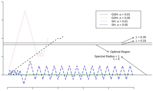
2.3 Heuristic Measures . . . 30
2.3.1 Search Heuristic . . . 30
2.3.2 Gradient Descent Heuristic . . . 30
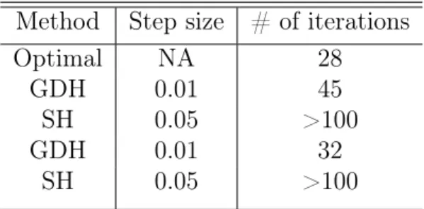
2.3.3 Comparing SH and GDH: A Concrete Example . . . 31
2.4 Asynchronous Message Updates . . . 32
2.5 Empirical Work . . . 35
2.5.1 Relaxed Gaussian Belief Propagation . . . 36
2.5.2 Compressed Inner-loop Convergence Fix . . . 40
2.5.3 Conjugate Gradient . . . 41
2.5.4 Further Empirical Considerations . . . 45
2.6 Conclusion . . . 46
3 Gaussian Belief Propagation with Nodes of Arbitrary Size 48 3.1 Preliminaries . . . 49
3.1.1 Notes on the Perron-Frobenius Theorem . . . 49
3.2 Constructing UWTs . . . 51
3.2.1 Topology of a UWT . . . 52
3.2.2 Specifying the Precision and Potential . . . 53
3.3 Analytical Formulas for the Posterior Means and Posterior Pre-cisions . . . 56
3.3.1 Tree-pruning Procedure . . . 56
3.3.2 UWT Correctness . . . 60
3.4 Automatic Preconditioning . . . 63
3.5 Exploiting the Tree and Line Topology . . . 65
3.5.1 Convergence of the Posterior Means . . . 66
3.5.2 Convergence of the Posterior Variances . . . 67
3.6 Convergence and Preconditioning . . . 69
3.7 Using UWTs for Messages . . . 71
3.8 Empirical Results . . . 72
3.8.1 Preconditioned Walk-summability . . . 72
3.8.2 Automatic Preconditioning . . . 73
3.9 Conclusion . . . 76
4 Higher-dimensional Regularised Gaussian Belief Propagation 77 4.1 Preliminaries . . . 77
4.1.1 UWT for the Precision Components . . . 78
CONTENTS x
4.2 Convergence of sGaBP . . . 79
4.2.1 Asymptotic Expressions . . . 79
4.2.2 Convergence to Linear Updates . . . 83
4.2.3 The Asymptotic Linear Update Matrix . . . 86
4.3 Adaptive Damping and Inference Quality . . . 87
4.4 Heuristic Regularisation . . . 88
4.4.1 Tree Representation of sGaBP . . . 88
4.4.2 Matrix Notation . . . 89
4.4.3 Recursive Representation of the Posterior Means . . . 90
4.4.4 Heuristic Regularisation . . . 90
4.5 Empirical Results . . . 92
4.5.1 Comparison of sGaBP with Other Methods . . . 93
4.5.2 Performance of Heuristic Regularisation . . . 95
4.5.3 Further Empirical Considerations . . . 97
4.6 Conclusion . . . 99
5 Conclusion 100 5.1 Selection of the Degree of Regularisation . . . 101
5.2 Multiple Regularisation Parameters . . . 101
5.3 Linear Systems and Distributive Application . . . 102
5.4 Extensions to Other Graph Types . . . 103
5.5 Novel Applications of GaBP . . . 104
Appendices 106 A Proofs for Chapter 2 107 A.1 Proof of Theorem 1 . . . 107
A.2 Proof of Theorem 2 . . . 107
A.3 Proof of Theorem 3 . . . 113
A.4 Simulation Information . . . 114
A.4.1 Simulation Scheme . . . 114
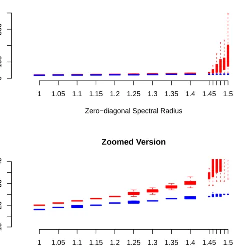
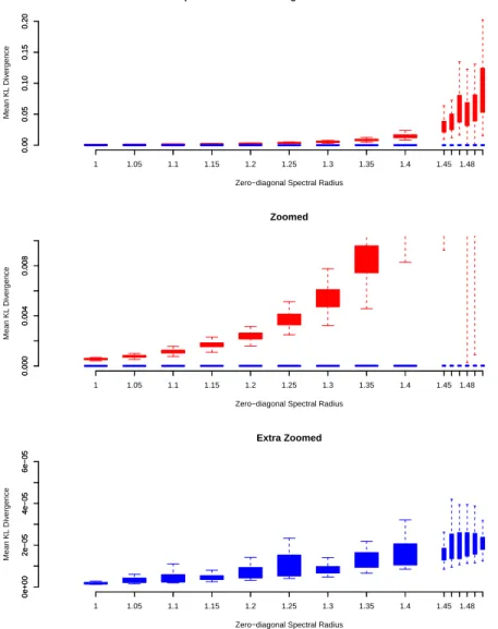
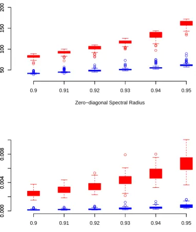
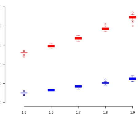
A.4.2 Regulating the Zero-diagonal Spectral Radius . . . 115
B Proofs for Chapter 3 116
C Proofs for Chapter 4 121
D Chapter 4 - Additional Notes 127
List of Figures
1.1 Examples of Markov Graphs. . . 2
1.2 Examples of clustered Markov Graphs. . . 3
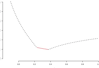
2.1 Plot of spectral radius as a function of λ. . . 29
2.2 Comparison of SH and GDH. . . 33
2.3 Comparison of the convergence speed of sGaBP and RGaBP. . . 37
2.4 Comparison of the inference quality of sGaBP and RGaBP. . . 38
2.5 Comparison of sGaBP and RGaBP in relaxation setting. . . 39
2.6 Comparison of the convergence speed of sGaBP and CFGaBP. . . . 42
2.7 Comparison of the inference quality of sGaBP and CFGaBP. . . 43
2.8 Comparison of the convergence speed of sGaBP and CG. . . 44
2.9 Trace Comparison of RGaBP, sGaBP and CG. . . 47
3.1 Different graph representations of a MG. . . 53
3.2 Visualisation of the process used to invert a tree-structured precision. 57 3.3 Visualisation of the results of simulations regarding preconditioning. 75 4.1 Comparison of the number of iterations required for convergence by sGaBP, CFGaBP and RGaBP. . . 95
4.2 Comparison of inference quality of sGaBP, CFGaBP and RGaBP. . 96
4.3 Illustration of performance of the heuristic method with different initialisations. . . 97
4.4 Trace Comparison of RGaBP, sGaBP. . . 98
D.1 Loopy Markov graph and the UWT for cluster 4 with a depth of n= 4. . . 130
List of Tables
2.1 Comparison of SH and GDH . . . 31
List of Abbreviations
BP belief propagation. ii, 1, 4–8, 12, 16, 28, 32, 41, 76, 100, 102–105
CFGaBP convergence fix Gaussian belief propagation. xi, 14–16, 40–43, 92–
96
CG conjugate gradient. ii, iv, xi, 22, 35, 42–47, 64, 72–76, 102, 103 FGaBP feedback Gaussian belief propagation. 14, 15
FMP feedback message passing. 14, 15
GaBP Gaussian belief propagation. ii, iii, viii, x, 6–19, 21, 22, 25, 29, 32, 33,
35, 36, 38, 40–42, 46, 48, 50, 51, 63–65, 69–76, 78, 79, 88, 93, 94, 96, 100–105, 114, 117
GDH gradient descent heuristic. xi, 30–33, 45
KL Kullback-Leibler. 29, 35–38, 40, 41, 43, 44, 46, 94, 95, 103, 104
MG Markov graph. ii, iii, xi, 1–5, 7, 8, 12, 13, 46, 48, 49, 51–54, 56, 70, 72,
77, 100, 103, 127
PCG preconditioned conjugate gradient. 72–74, 102, 103 PGM probabilistic graphical model. 1, 4
ReGaBP reweighted Gaussian belief propagation. 14
RGaBP relaxed Gaussian belief propagation. xi, 15, 16, 36–40, 45–47, 87,
92–98
RIP running intersection property. 104
sGaBP slow Gaussian belief propagation. x, xi, 16–18, 20–25, 27–32, 34–47,
77–79, 83, 85, 87–90, 92–105, 114, 127
SH search heuristic. xi, 30–33
LIST OF ABBREVIATIONS xiv
UWT unwrapped trees. ix, xi, 46, 48, 51–56, 60, 64–66, 68, 70, 71, 76, 78–80,
Chapter 1
Introduction
The main goal of this chapter is to provide the reader with a high-level under-standing of the topics covered in this dissertation before delving into specifics in the subsequent chapters. The scope can be narrowed to the application of belief propagation (BP) to probabilistic graphical models (PGMs). We start with a discussion of these fundamentals.
1.1
Probabilistic Graphical Models
PGMs are used to represent the conditional dependence between random vari-ables in the form of a graph. PGMs can be used to encode complex probability distributions compactly and allow the user to exploit the conditional depen-dence structure of a random vector to perform tasks efficiently (even in some otherwise intractable tasks). Consider for instance the task of assigning val-ues to a vector of binary random variables X : k×1 given evidence E. The maximum a posteriori (MAP) assignment is
xMAP =argmax
x
{Prob(X=x|E)}, (1.1) where x= (x1, x2, . . . , xk)0 is such that xi ∈ {0,1}. The brute-force approach
would be to evaluate Prob(X =x|E) for all 2k possible x, a computationally intractable task even for moderatek. A PGM would attempt to exploit condi-tional independence characteristics of Prob(X=x|E)to perform the inference
given in Equation (1.1) in a tractable way, using one of a variety of algorithms. In this dissertation we focus on Markov graphs (MGs), also known as undi-rected graphs or Markov random fields. A MG consists of a set of nodesV and
a set of edgesE. Each node inV is represented by a random variable, while the
set of edgesE defines which nodes are linked in the graph. Consider two nodes
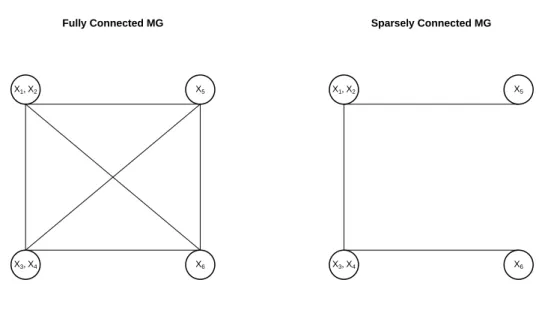
i, j, where i6=j, and let m =min(i, j) and n = max(i, j). Nodes i and j are linked if and only(m, n)∈ E. Figure 1.1 contains two examples of a MG for the
random vectorX= (X1, X2, X3, X4, X5, X6)0. The set of edges for the sparsely 1
CHAPTER 1. INTRODUCTION 2 Fully Connected MG X1 X2 X3 X4 X5 X6 Sparsely Connected MG X1 X2 X3 X4 X5 X6
Figure 1.1: Illustration of two MGs for the random vector X =
(X1, X2, X3, X4, X5, X6)0. The left side shows a fully connected MG, while the right side shows a sparsely connected graph.
connected graph in Figure 1.1 is E = {(1,2); (1,3); (2,5); (3,4); (4,6)}. The
neighbourhood of node i is denoted by Ni ={j : (i, j)∈ E} ∪ {j : (j, i)∈ E}.
For the fully connected graph in Figure 1.1, we have N3 ={1,2,4,5,6}, while
for the sparsely connected graph, N3 ={1,4}.
The structure of a MG can be used to infer certain conditional independen-cies of the random vector it represents. Consider a MG, G, for the random
vector X = (X1, X2, . . . , Xk)0. The univariate variables Xi, Xj, where i < j,
are conditionally independent given the other variables if (i, j)∈ E/ (these are called the pairwise independencies of the graph). In the sparsely connected graph of Figure 1.1, we see that the random variables X1 and X6 are
condi-tionally independent given the other random variables. Let X1, X2 and X3
be non-overlapping subvectors of X. The vectorsX1 and X2 are conditionally
independent givenX3 if every path between the nodes representingX1 and the
nodes representing X2 intersect a node representing a variable in X3. These
are called the global Markov independencies ofG. For instance, in the sparsely
connected graph of Figure 1.1, we see that the random variable X5 and the
Fully Connected MG X1, X2 X3, X4 X5 X6 Sparsely Connected MG X1, X2 X3, X4 X5 X6
Figure 1.2: Illustration of clustering applied to the two MGs displayed in Figure 1.1. The clusters are(X1, X2)0; (X3, X4)0;X5 and X6.
We also allow for MGs where nodes can receive more than one variable. Con-sider the partition X = (X01,X02, . . . ,Xp0)0, where Xt : t = 1,2, . . . , p are
non-overlapping subvectors of X. Suppose we are interested in the pairwise inde-pendencies of these subvectors, i.e. are Xt and Xs conditionally independent,
given the other subvectors? From the global Markov independencies we can define a new graph, G˜, with nodes V˜ = {1,2, . . . , p} and (s, t) ∈ E˜ if, and
only if, no variable in Xs has a edge with a variable in Xt inG. The pairwise
independencies of the partition can be inferred fromG˜in the same way we
in-ferred the pairwise independencies of the univariate random variables from G.
We refer to the process of creating a partition as clustering. When confronted with clustering, the term MG refers to G˜. The MGs for the graphs displayed
in Figure 1.1, with the clusters (X1, X2)0; (X3, X4)0;X5 and X6, are given in
Figure 1.2. For the sparsely connected graph, we see that (X1, X2)andX6 are
conditionally independent given the other variables. This figure also displays the assertion that the random variable X5 and the random vector (X3, X4)0
are conditionally independent given (X1, X2)0 more clearly.
When performing clustering, we denote the indices of the variables repre-sented by cluster i as Ci. For the clustering done in Figure 1.2 we see that C1 = {1,2},C2 = {3,4},C3 = {5} and C4 = {6}. Let vec(Ci) be the vector of
CHAPTER 1. INTRODUCTION 4
(vec(C1)0,vec(C2)0, . . . ,vec(Cp)0)0 = (1,2, . . . , k)0 (if this does not hold the
vari-ables can be reordered to do so).
In the next section we discuss a certain type of BP that exploits the pair-wise and global independencies of MGs to obtain computational advantages for the task of performing inference.
1.2
Belief Propagation
Belief propagation (BP) is one of the algorithms that can be used to perform inference on PGMs. Informally speaking, BP is a message-passing algorithm that communicates between the nodes of a PGM. The critical advantage is that direct communication between unlinked nodes is not necessary. Hence the more sparse the graph, the more efficient the BP. The BP algorithm itera-tively constructs messages between linked nodes until the messages converge. At this point a node collects all incoming messages and uses these to create a potential. This potential is used to perform inference.
In the context of error-correcting codes, the roots of BP can be traced back to the development of the sum-product algorithm as a decoding algorithm for LDPC codes (Gallager, 1963). Belief propagation (probability propaga-tion) for Bayesian networks was introduced by Pearl (1988); Shachter (1988); Shafer and Shenoy (1990); and Lauritzen and Spiegelhalter (1988). BP was found (at a later stage) to be equivalent to the sum-product algorithm (Frey and Kschischang, 1996; Aji and McEliece, 2000). Perhaps the most successful application of BP can be found in the development of turbo codes, with per-formances in terms of bit error rate (BER) approaching that of the Shannon limit (Murphy et al., 1999).
BP on tree-structured graphs is known to converge and provide exact infer-ence at converginfer-ence (Pearl, 1988). The inferinfer-ence quality of BP can be severely compromised when it is applied to loopy graphs (Weiss and Freeman, 2001). A graph is said to contain a loop if there exists a path in the graph that connects a node to itself. When a graph has loops, BP does not necessarily converge, and even if it does, is not guaranteed to provide exact inference. Even so, BP is useful in many applications due to its computational tractability, particu-larly in cases where the inference quality of BP is acceptable (as in the case of turbo codes).
In this dissertation we focus on BP applied to MGs where the underlying density function has a specific factorisation. We discuss this factorisation in the next section.
1.2.1
Formulation
Let us consider a random vector X : k×1 with density function f(x). Our
task is to perform inference on f(x) where it is assumed that,
f(x) = 1 Z Y i∈V ψii(xi) Y (i,j)∈E ψij(xi,xj), (1.2)
whereZ is a normalising constant, thexi’s are mutually exclusive and
exhaus-tive subvectors of x = (x01,x02, . . . ,x0p)0 and V = {1,2, . . . , p} where p ≤ k. Consider the MG obtained by partitioning X according to the partition x= (x01,x02, . . . ,x0p)0. A consequence of the Hammersley-Clifford theorem
(Ham-mersley and Clifford, 1971; Clifford, 1990) is that the MG for the partition will have nodes V and edges E. Note that if (i, j) ∈ E we implicitly assume
that i < j.
When the nodes are one-dimensional (p = k), the factorisation in Equation (1.2) yields a pairwise MG. There are many ways of formulating BP on the factorisation given in Equation (1.2) (factor graphs or cluster graphs, for ex-ample). In this dissertation we focus on a multivariate extension of BP on pairwise MGs.
Let Ni\j be the setNi with element j removed (the assumption thatj ∈ Ni
is made implicitly). BP can be formulated using the sum-product or max-sum rule. For the max-sum-product rule, BP seeks to perform iterative updates to obtain the stationary conditions,
mij(xj) = Z ψii(xi)ψij(xi,xj) Y t∈Ni\j mti(xi)dxi, (1.3)
for all i∈ V and allj ∈ Ni. For the max-sum rule, this changes to
mij(xj) =max xi log(ψii(xi)) +log(ψij(xi,xj)) + X t∈Ni\j mti(xi) , (1.4) for all i ∈ V and all j ∈ Ni. Note that the max-sum formulation given
in Equation (1.4) can easily be changed to a minimisation problem. In both Equation (1.3) and Equation (1.4) we haveψij(xi,xj) = ψji(xj,xi)wheni > j.
1.2.2
Message Updates
Bickson (2008) describes two conventional types of message-update rules that can be used for the purpose of iterating equations to achieve the stationary conditions given in Equation (1.3) or Equation (1.4). In synchronous message passing, new messages are formed using messages from the previous round only
CHAPTER 1. INTRODUCTION 6
and are therefore not influenced by the message scheduling. This is in con-trast to the asynchronous case, where messages updated in the current round are used to compute new messages. Although asynchronous updates tend to outperform the synchronous approach (Koller and Friedman, 2009), our main focus is on the synchronous case. We do this since one of the more attractive properties of GaBP is its application in distributive settings, which is far more compatible with synchronous message updates. Synchronous implementation also allows us to compare different GaBP algorithms without considering the effects of different message schedulings. For the sum-product formulation, the synchronous message updates will be,
m(ijn+1)(xj) = Z ψii(xi)ψij(xi,xj) Y t∈Ni\j m(tin)(xi)dxi, (1.5)
while for the max-sum we have: m(ijn+1)(xj) = max xi log(ψii(xi)) +log(ψij(xi,xj)) + X t∈Ni\j m(tin)(xi) , (1.6) for alli∈ V and allj ∈ Ni. The sum-product and max-sum formulation of BP
are related in the sense that they can both be used to perform approximate inference, although they may provide different approximations. We note that if the density function given in Equation (1.2) is a Gaussian density function, then the message updates given in Equations (1.5) and (1.6) are equivalent.
1.2.3
Posterior Distributions
We associate with each i ∈ V the prior distribution ψii(xi). After iteration n
we have messages m(ijn)(xj) for all i∈ V and allj ∈ Ni. Within the context of
BP, we can construct a posterior distribution for node i at iterationn using post(n) i (xi) =ψii(xi) Y t∈Ni m(tin)(xi) (1.7) and post(n) i (xi) = ψii(xi) Y t∈Ni exp m(tin)(xi) . (1.8)
for the sum-product and max-sum formulations respectively. Essentially, the distribution given in Equation (1.7) (or Equation (1.8)), after appropriate nor-malisation, provides an approximation for the true marginal density function of the variables in xi. Consider the max-sum formulation and let
post(n) i\j(xi) = ψii(xi) Y t∈Ni\j exp m(tin)(xi) , (1.9)
then
m(ijn+1)(xj) =max xi
log(post(in\j)(xi)) +log(ψij(xi,xj))
. (1.10) Equation (1.10) provides a good basis for motivating our high-level approach, which we discuss in the next section.
1.2.4
High-level Approach of this Dissertation
The focus of this dissertation can be (partially) narrowed to addressing the convergence shortcomings of BP when applied to loopy MGs. The idea is to develop an adjusted BP variant that is able to perform satisfactory inference on loopy MGs with an arbitrary conditional independence structure. To this end we propose a regularised variant of Equation (1.6) (we give a sum-product variant in Section 1.4.3): m(ijn+1)(xj) =max xi log(ψii(xi)) +log(ψij(xi,xj)) + X t∈Ni\j m(tin)(xi) − λ q||xi−θ (n−1) i || q q =max xi log(post(i\nj)(xi))− λ q||xi −θ (n−1) i || q q+log(ψij(xi,xj)) (1.11) The valueθi(n−1) in Equation (1.11) is selected at iterationn−1, andλis a reg-ularisation parameter. Essentially we are encouraging xi to take values closer
to θ(in−1) at iteration n for the purpose of constructing the messages to neigh-bouring nodes at iteration n+ 1. The purpose of the max-sum variant given in
Equation (1.11) is to provide a method that will converge for any MG, while providing satisfactory inference quality. In cases where basic BP converges, this method should provide comparable results (hopefully improving), both in terms of convergence speed and inference quality. This dissertation focuses on discussing these aspects for a special MG, i.e. one induced by a multivariate Gaussian distribution. The Gaussian assumption simplifies certain technical aspects (such as conjugacy of the messages) and provides a convenient start-ing point for teststart-ing our high-level approach. It is our viewpoint that, if the propagation given in Equation (1.11) proves successful for the Gaussian case, there is no reason why it should not be able to generalise to other MGs and indeed general BP on graphs.
BP on a MG induced by a multivariate Gaussian distribution is often referred to as Gaussian belief propagation (GaBP). On a high level, this dissertation is concerned with addressing the problems underlying the application of BP to
CHAPTER 1. INTRODUCTION 8
general loopy MGs using the Gaussian assumption as an example. It should be noted that studying GaBP is worthwhile in its own right and there is signif-icant literature available on this subject. This is reviewed in the next section. Although this dissertation is focused heavily on GaBP, we do not want the reader to forget the high-level approach and the link to BP in general. We highlight some focus points of this dissertation:
• Providing mathematical details and proofs for validating our high-level approach (such as proving convergence).
• Providing empirical evidence for statements not explicitly proven. • Empirical comparisons of our GaBP variant with other variants from the
literature.
• Proposing novel ways of utilising the GaBP algorithm.
In the next section we discuss aspects of GaBP and conduct a literature review of the topic.
1.3
Gaussian Belief Propagation
GaBP is a specialised application of BP on a Markov graph assuming a mul-tivariate Gaussian random variable in canonical parameterisation. From this point onwards we denote the precision matrix of a k ×1 Gaussian random
variable by S : k×k and the potential vector by b : k×1. Consider the set
of nodes V where |V| = p≤ k. Each node i in V is associated with a cluster
of variables Ci ⊆ {1,2, . . . , k}, such that the Ci’s are mutually exclusive and ∪i∈VCi ={1,2, . . . , k}.
Notation 1 Consider the precision matrix S and the clusters C1,C2, . . . ,Cp
assigned to nodes. Set di =|Ci|. By Sij : di×dj we mean the submatrix of S
corresponding to the variables in Ci for the rows and Cj for the columns. The
vector bi :di ×1 is the subvector of b corresponding to the variables in Ci.
Notation 2 For a Gaussian distribution with precision matrix S, the set of edges is defined to be E ={(i, j) : i < j and Sij 6= 0}. The neighbourhood of
node i simplifies to Ni ={j =6 i:Sij 6=0}.
In terms of Equation (1.2) we can write: ψii(xi) =exp −1 2x 0 iSiixi+x0ibi :i∈ V ψij(xi,xj) =exp −x0iSijxj : (i, j)∈ E. (1.12)
We can now apply the max-sum rule to formulate the message updates for the GaBP algorithm. The max-sum and sum-product rules are equivalent in the Gaussian case. See, for instance, Bickson (2008) for the equivalence of sum-product GaBP and max-sum-product GaBP (identical to max-sum) where nodes are one-dimensional. A proof for this equivalence in the multivariate case is given implicitly in Section 1.4.3 (the proof can be obtained by setting λ = 0
in the derivation).
1.3.1
Message Updates
We proceed under the assumption thatm(ijn)(xj) = K (n) ij − 1 2x 0 jQ (n) ij xj+x0jv (n) ij ,
Kij(n) is a constant andQ(ijn) :dj×dj is symmetric for all nodesiand allj ∈ Ni.
We have that log(post(in\j)(xi)) =− 1 2x 0 iSiixi+x0ibi+ X t∈Ni\j Kti(n)− 1 2 X t∈Ni\j x0iQ(tin)xi + X t∈Ni\j x0iv(tin) =−1 2x 0 i Sii+ X t∈Ni\j Q(tin) xi+x0i bi+ X t∈Ni\j v(tin) + ˜Kij(n) =−1 2x 0 iP (n) ij xi+x0iz (n) ij + ˜K (n) ij , (1.13) whereP(ijn)=Sii+Pt∈Ni\jQ (n) ti ,z (n) ij =bi+Pt∈Ni\jv (n) ti andK˜ (n) ij = P t∈Ni\jK (n) ti .
We make the additional assumption thatP(ijn)is positive definite and note that P(ijn) is symmetric by the symmetry of the Q(tin)’s. We see that:
m(ijn+1)(xj) = ˜K (n) ij +max xi −1 2x 0 iP (n) ij xi+x0i(z (n) ij −Sijxj) = ˜Kij(n)+1 2(Sijxj −z (n) ij ) 0 [P(ijn)]−1(Sijxj−z (n) ij ) = ˜Kij(n)+1 2[z (n) ij ] 0 [P(ijn)]−1z(ijn)+ 1 2x 0 jSji[P (n) ij ] −1S ijxj −x0jSji[P (n) ij ] −1 z(ijn) =Kij(n+1)− 1 2x 0 jQ (n+1) ij xj+x0jv (n+1) ij , (1.14) where: Kij(n+1) = ˜Kij(n)+1 2[z (n) ij ] 0 [P(ijn)]−1z(ijn) Q(ijn+1) =−Sji[P (n) ij ] −1S ij (1.15) vij(n+1) =−Sji[P (n) ij ] −1z(n) ij . (1.16)
CHAPTER 1. INTRODUCTION 10
We see that conjugate messages can be obtained through appropriate initiali-sation and we use Q(0)ij =0 and vij(0) =0 for all nodesi and all j ∈ Ni.
1.3.2
Processing the Posteriors
After performing one pass of synchronous message updates we need to con-struct marginals associated with the updated messages. At iteration n we have: post(n) i (xi) = ψii(xi) Y t∈Ni exp m(tin)(xi) =exp − 1 2x 0 iSiixi+x0ibi Y t∈Ni exp Kti(n)−1 2x 0 iQ (n) ti xi+x0iv (n) ti =exp X t∈Ni Kti(n) exp − 1 2x 0 iP (n) i xi+x0iz (n) i ∝exp − 1 2x 0 iP (n) i xi+x0iz (n) i , where P(in) = Sii+Pt∈NiQ (n) ti and z (n) i = bi +Pt∈Niv (n)
ti . Notice that the
constantKij(n)plays no role in determining the marginal after the posterior dis-tribution has been normalised. Hence the update and tracking of the constant component of the messages is ignored in the GaBP algorithm. Note that the posterior distribution estimates the marginal as a Gaussian distribution, with precision matrix and potential vector P(in) and z(in) respectively. This gives an estimate for the marginal mean, i.e. µ(in) = [Pi(n)]−1z(n)
i , and therefore we
can use the GaBP algorithm to convert a multivariate Gaussian distribution in canonical form to approximate marginals in the mean-covariance param-eterisation. This is an important observation, since it links GaBP to linear algebra. We introduce some terminology:
Terminology 1 The posterior distribution for node i ∈ V resulting from the GaBP algorithm at iteration nis characterised by the posterior precision, P(in), and the posterior mean, µ(in).
The synchronous GaBP procedure in Algorithm 1 uses the following compu-tational shortcuts:
Pij(n)=Pi(n)−Q(jin) zij(n)=zi(n)−v(jin).
Algorithm 1 is terminated when Err ≤ , where e(in) = P
jSijµ
(n)
j −bi and
Algorithm 1 Synchronous GaBP
1. Provide a precision matrix S : k×k, a potential vector b : k×1 and
clusters Ci :i= 1,2, . . . , p as inputs.
2. Specify a tolerance and a maximum number of iterations m. 3. Initialise Q(0)ij =0:dj×dj and v
(0)
ij =0:dj×1 for all i and allj ∈ Ni.
4. Set Err=Inf andn = 0.
5. While Err> a) Compute P(in) = Sii+ P j∈NiQ (n) ji and z (n) i = bi + P j∈Niv (n) ji for i= 1,2, . . . , p. b) Set µ(in) = [Pi(n)]−1z(n) i , e (n) i = P jSijµ (n) j − bi and Err = maxi{||e(in)||∞}.
c) If Err> , do for all i∈ {1,2, . . . , p} and all j ∈ Ni:
Q(ijn+1) =−Sji[P(in)−Q (n) ji ] −1S ij and v(ijn+1) =−Sji[P (n) i −Q (n) ji ] −1[z(n) i −v (n) ji ]. d) Increment n. e) If n =m, break. 6. End.
reason for this is that convergence of the posterior means usually indicates that the remaining components of the algorithm have converged, since the posterior means are functions of all the components iterated in Algorithm 1. In the next section we discuss the convergence and inference quality of the GaBP algorithm.
1.3.3
Convergence Behaviour and Inference Quality
Important work on GaBP can be found in Weiss and Freeman (2001). Here it is shown that, if GaBP converges, the marginal means supplied by this algorithm are the correct ones. Furthermore, it is shown that, if the precision matrix is strictly diagonally dominant, GaBP is guaranteed to converge.Definition 1 A matrix S= [sij] is defined to be strictly diagonally dominant
(sdd) if sii >Pj6=i|sji| for all i.
Definition 2 A matrix S= [sij] is defined to be weakly diagonally dominant
CHAPTER 1. INTRODUCTION 12
Weiss and Freeman (2001) also interpret GaBP on loopy graphs as BP on a tree-structured Gaussian MG (known as unwrapped trees). This provides a more convenient typology for the convergence analysis of GaBP, something that will be revisited in this dissertation.
Unfortunately, GaBP does not necessarily provide the correct marginal pre-cisions at convergence, but can still provide reasonable estimates for these quantities.
The exact convergence properties of GaBP remains an open area of research. The class of precision matrices for which GaBP converges has been expanded to include precision matrices that are walk-summable (Malioutovet al., 2006). We introduce some new notation and definitions.
Notation 3 Consider a matrix A : m×n. By |A| we mean the matrix A in which all elements are replaced by their corresponding absolute values. The determinant of a square matrix A is denoted by det(A).
Definition 3 Consider a matrix A : m×m with eigenvalues (possibly com-plex) λ1, λ2, . . . , λm. Let |.| be the modulus of a complex number. The spectral
radius of A is defined as maxi{|λi|} and is denoted by ρ(A).
Definition 4 The zero-diagonal spectral radius of a matrix A:m×m = [aij]
is defined to be the spectral radius of diag(a11, a22, . . . , amm)−A, and is denoted
by ρ˜(A).
Definition 5 Consider a positive definite matrix S : p ×p = [sij] and let
D = diag(√1 s11, 1 √ s22, . . . , 1 √
spp). The matrix S is defined to be walk-summable
if ρ˜(|DSD|)<1.
The proof for convergence of the GaBP algorithm for walk-summable preci-sion matrices provided by Malioutov et al. (2006) is for univariate nodes. In Chapter 3 we show that the walk-summability convergence result also extends to the multivariate case. We will also define a new, preconditioned variant of walk-summability that shows that GaBP with higher-dimensional nodes could converge in cases where the univariate version does not. A recent work provides necessary and sufficient conditions for the convergence of univariate synchronous GaBP, under a specified initialisation set (Su and Wu, 2015). Furthermore, necessary and sufficient convergence conditions are established for damped univariate synchronous GaBP and these include the allowable range for the damping factor. They also provide theoretical confirmation that damping can improve the convergence behaviour of GaBP. The problem with these contributions is that their conditions for convergence may be difficult to verify. For instance, verifying walk-summability requires finding the maxi-mum absolute eigenvalue of a p×p matrix, while the conditions from Su and
Wu (2015) require solving a semi-definite program (SDP) and evaluating the spectral radius of an infinite dimensional matrix (Sui et al., 2015).
1.3.4
Links to Linear Algebra
GaBP can be connected to the area of linear algebra (Shentalet al., 2008). As discussed previously, GaBP can be used to convert a multivariate Gaussian dis-tribution in canonical form to approximate marginals for each set of variables
Ci : i = 1,2, . . . , p. Suppose that GaBP has converged, then the converged
posterior marginals provide the exact marginal means, i.e. µ(i∞) =µi, where
Sµ=b, and hence GaBP implicitly solves this linear system of equations. The
use of GaBP as a solver of linear systems has been proposed in the literature (Shentalet al., 2008; Bickson, 2008; El-Kurdiet al., 2012b). GaBP is attractive as a solver of linear systems due to the ease of distributed implementation and the exploitation of sparsity in the precision matrix (our high-level approach retains these characteristics).
One of the major restrictions in using GaBP as a solver of linear systems is that it can only be applied on a sub-class of symmetric and positive defi-nite matrices. In this dissertation, we will show that our high-level approach yields a GaBP variant capable of converging for any symmetric and positive definite matrix, given sufficient regularisation. Hence, our approach expands the application domain of GaBP in the context of linear systems.
GaBP has been compared favourably to other solvers of linear systems in the literature, such as the Jacobi and Gauss-Seidel methods (Bickson, 2008). In our experience, the GaBP algorithm can struggle to compete with methods such as the conjugate gradient (CG) and preconditioned conjugate gradient (PCG) methods, particularly in loopy MGs with ill-conditioned precision ma-trices. Apart from inducing convergence, our high-level approach can also accelerate GaBP in cases where this algorithm converges without the aid of regularisation. A portion of this dissertation is dedicated to comparing our GaBP variant with the CG and PCG methods for the purpose of solving lin-ear systems. In Chapter 3 we show that the basic GaBP algorithm performs a certain type of preconditioning automatically. The fact that this precondi-tioning can significantly lower the condition number of the precision matrix is an advantage of GaBP over CG and PCG.
From a marginalisation viewpoint, GaBP can be used to estimate the marginal precision associated with each set of variables assigned to nodes. The direct method of determining the marginal precisions is to invert the precision ma-trix, extract the appropriate blocks and invert these block matrices. Therefore, GaBP can be used for the purpose of estimating certain diagonal blocks of the inverse of symmetric and positive definite matrices without the use of direct
CHAPTER 1. INTRODUCTION 14
matrix inversion. Within the context of our high-level approach, we show, empirically, that its application in GaBP can often improve the accuracy of these approximations.
1.3.5
Competing Algorithms
This section is dedicated to describing some of the competing algorithms to our approach.
• Convergence Fix GaBP - CFGaBP (Johnsonet al., 2009). This method uses basic GaBP to solve a sequence of linear systems defined by (S+
λI)µ(n) = b+ λµ(n−1). If λ is chosen sufficiently large (for instance,
large enough forS+λIto be walk-summable), each application of basic GaBP will converge and the limit of µ(n) will solve the system of
equa-tions Sµ=b.
One problem with CFGaBP is that convergence can be slow due to the double-loop nature of the algorithm (inner loop applies GaBP and outer loop updates the linear system). Also, since CFGaBP was designed specifically to solve linear systems, it does not address the problem of improving the precision estimates.
• Reweighted GaBP - ReGaBP (Ruozzi and Tatikonda, 2013). This ap-proach uses a parameterised generalisation of the max-sum algorithm to improve on the convergence of GaBP. For ReGaBP there is always a set of parameters that gives computation trees that are positive definite – this is sufficient for the precision components of messages to converge. The main problem with ReGaBP is that it may require additional damp-ing factors for the mean components to converge. As far as we are aware, there are no theoretical results establishing that there will always be suf-ficient damping to guarantee convergence (although we were always able to find sufficient damping in our simulations). In our opinion, the con-vergence behaviour of ReGaBP can be erratic in terms of the selection of the reweighting, and this is further complicated by the need for ad-ditional damping. The effect of the reweighting of the messages on the accuracy of the posterior precisions as approximations for the marginal precisions is a concern.
• Feedback GaBP - FGaBP (Liu, 2010). A set of nodes is called a feed-back set if their removal results in a cycle-free graph. The individual nodes in such a set are called feedback nodes. The idea behind a feed-back message passing algorithm (FMP) is to treat the feedfeed-back and non-feedback nodes separately. Informally speaking, a FMP starts with mes-sage passing among the non-feedback nodes. The non-feedback nodes
send messages to the feedback nodes, which they use to compute their exact marginals. The next step is for the feedback nodes to pass mes-sages, based on their exact marginals, back to the non-feedback nodes. The non-feedback nodes use these messages to perform a final round of message-passing, yielding their exact marginals.
For the Gaussian case, the inference provided by a FMP is exact and completes after O(k2p) computations, with k being the number of
feed-back nodes and p the total number of nodes. The consequence is that we would like the feedback set to be as small as possible.
The main problem with FGaBP is that it is less applicable in graphs with a low degree of sparsity. When a graph has a low degree of sparsity, the size of the smallest feedback set will be large, resulting in a higher number of computations. Furthermore, even in cases of moderate spar-sity, finding the smallest feedback set can be computationally intractable. One way of dealing with these issues is to use a pseudo-feedback set, that is a set of nodes the removal of which removes the most significant cy-cles in the graph. The advantage is that the pseudo-feedback set can be chosen to be of any size. The disadvantages are that inference be-comes approximate and one is still left with the task of selecting a good pseudo-feedback set.
• Relaxed GaBP - RGaBP (El-Kurdi et al., 2012b). RGaBP uses relax-ation factors (algorithm can easily be adjusted to use damping factors) to accelerate the convergence of basic GaBP (Su and Wu, 2015).
The main problem with RGaBP is that it uses the same updates as basic GaBP for the precision components of messages. The consequence is that RGaBP cannot be applied to arbitrary precision matrices. • Johnson et al. (2009) make a brief reference to a compressed inner-loop
version of CFGaBP, in which each application of GaBP is limited to one iteration. They report that compressed inner-loop CFGaBP can be more efficient than the original method, but may require damping for the adjustment of the potential vector.
The similarity of the compressed CFGaBP to our algorithm depends heavily on the interpretation of the description in the literature. We could not find any reference to compressed CFGaBP in the source code provided by Bickson (2008). If we consider the source code provided for the original CFGaBP method, and apply the description provided by Johnson et al. (2009), we see differences in the application of the two methods.
CHAPTER 1. INTRODUCTION 16
In contrast to the method provided in this dissertation, compressed inner-loop CFGaBP is not a full marginalisation algorithm, requires additional damping factors to be specified, is not theoretically proved to converge for all precision matrices, is not generalised to higher-dimensional nodes, and does not provide a principle that can be applied in general BP. Each algorithm mentioned above suffers from at least one of the following problems:
1. Does not provide a principle that can be generalised to other applications of BP.
2. Does not converge for arbitrary precision matrices. 3. Convergence can be slow due to implementation method. 4. Estimation of the precisions is ignored.
5. No theoretical proof of guaranteed convergence. 6. Not applicable in dense graphs.
7. Focus is on one-dimensional nodes only.
A large portion of this dissertation will be dedicated to show how our algorithm deals with these issues. In the empirical sections of Chapter 2 and Chapter 4, we provide a comparison of our variant with some of these algorithms. The next section describes the application of our high-level approach in GaBP.
1.4
High-level Application in GaBP
We refer to the application of our high-level approach in GaBP as “regularised” - or “slow” - Gaussian belief propagation. The “slow” relates the regularisation used in our approach to the principle of slow learning. We label our method sGaBP as opposed to rGaBP to avoid confusion with relaxed Gaussian belief propagation (RGaBP).
1.4.1
Message Updates
A natural selection for the Lq-norm in Equation (1.11) is q = 2, since this
will preserve the conjugacy. As for GaBP, we assume that m(ijn)(xj) = Kij(n)− 1 2x 0 jQ (n) ij xj +x0jv (n)
ij , where the components will depend on λ. We will not
express the dependence on λ explicitly. Again, Kij(n) is a constant and Q(ijn) is symmetric. In an identical manner to Equation (1.13), we obtain:
log(post(i\nj)(xi)) =− 1 2x 0 iP (n) ij xi+x0iz (n) ij + ˜K (n) ij . (1.17)
The application of Equation (1.11) yields: m(ijn+1)(xj) = ˜K (n) ij +maxx i −1 2x 0 iP (n) ij xi+x0i(z (n) ij −Sijxj) − λ 2(xi−θ (n−1) i ) 0 (xi−θ (n−1) i ) = ˜Kij(n)− λ 2[θ (n−1) i ] 0 θi(n−1) +max xi −1 2x 0 i(P (n) ij +λIdi)xi+x 0 i(z (n) ij +λθ (n−1) i −Sijxj) =K˜˜ij(n) +1 2(Sijxj −z (n) ij −λθ (n−1) i ) 0 [P(ijn)+λIdi] −1(S ijxj −z (n) ij −λθ (n−1) i ) =K˜˜ij(n)+1 2[z (n) ij +λθ (n−1) i ] 0 [P(ijn)+λIdi] −1[z(n) ij +λθ (n−1) i ] +1 2x 0 jSji[P (n) ij +λIdi] −1S ijxj −x0jSji[P (n) ij +λIdi] −1[z(n) ij +λθ (n−1) i ] =Kij(n+1)− 1 2x 0 jQ (n+1) ij xj +x0jv (n+1) ij , (1.18) where: ˜ ˜ Kij(n) = ˜Kij(n)− λ 2[θ (n−1) i ] 0 θ(in−1) Kij(n+1) =K˜˜ij(n)+1 2[z (n) ij +λθ (n−1) i ] 0 [P(ijn)+λIdi] −1[z(n) ij +λθ (n−1) i ] Q(ijn+1) =−Sji[P(ijn)+λIdi] −1 Sij v(ijn+1) =−Sji[P(ijn)+λIdi] −1 [z(ijn)+λθ(in−1)].
We still have not discussed the selection of the value θ(in−1). Suppose that
the posterior distribution associated with node i at iterationn−1 is given by
post(n−1)
i (xi), then we propose using: θi(n−1) =argmax
xi
{post(in−1)(xi)}. (1.19)
In the next section we will see that post(n−1)
i (xi)is proportional to a Gaussian
distribution and hence,
θi(n−1) =µ(in−1). (1.20)
1.4.2
Processing the Posteriors
Normal GaBP gives the correct marginal means under the assumption of con-vergence. In order to preserve this property for sGaBP, we need to treat the
CHAPTER 1. INTRODUCTION 18
posterior distributions in a slightly different way than for GaBP. We form the posterior distribution at iteration n as:
post(n) i (xi)∝exp −1 2x 0 iP (n) i xi+x0iP (n) i [λIdi+P (n) i ] −1[z(n) i +λµ (n−1) i ] (1.21) where P(in) = Sii +Pt∈NiQ (n) ti and z (n) i = bi + Pt∈Niv (n) ti . The precision
associated with Equation (1.21) is similar to the precision associated with GaBP, howeverQ(tin)now depends on the regularisation parameter. For clarity we note that post(n)
i\j(xi) remains ψii(xi) Y t∈Ni\j exp m(tin)(xi)
as in Equation (1.9), but now depends on λ. The marginal mean associated with Equation (1.21) can be shown to be:
µ(in) = [λIdi+P
(n)
i ]
−1
[z(in)+λµ(in−1)]. (1.22) Essentially we are introducing a form of damping on the progression of the posterior means over the iterations. This damping is necessary to ensure that the posterior means provided at convergence give the correct marginal means (see Theorems 3 and 14).
We implement sGaBP in Algorithm 2 (see next page), where we use the nota-tion:
P(in)(λ) =λIdi+P
(n)
i .
1.4.3
Sum-product sGaBP
In this section we discuss a sum-product (as opposed to max-sum) formulation of sGaBP. The sum-product message updates in the unregularised setting was given as, m(ijn+1)(xj) = Z ψii(xi)ψij(xi,xj) Y t∈Ni\j m(tin)(xi)dxi,
in Equation (1.5). Within the context of regularisation, we define the message-updates to be: m(ijn+1)(xj) = Z ψii(xi)ψij(xi,xj)exp − λ q||xi−θ (n−1) i || q q Y t∈Ni\j m(tin)(xi)dxi, (1.23)
Algorithm 2 Synchronous regularised GaBP
1. Provide a precision matrix S : k×k, a potential vector b : k×1 and
clusters Ci :i= 1,2, . . . , p as inputs.
2. Specify a tolerance, a maximum number of iterationsm and a regular-isation parameter λ.
3. Initialise Q(0)ij =0:dj ×dj,v (0)
ij =0:dj ×1,µ
(−1)
i =bi for all i and all
j ∈ Ni.
4. Set Err=Inf andn = 0.
5. While Err> a) Compute P(in)(λ) = λIdi+Sii+ P j∈NiQ (n) ji and z(in) =bi+Pj∈Niv (n) ji for i= 1,2, . . . , p. b) Set µ(in) = [Pi(n)(λ)]−1[λµi(n−1)+z(in)], e(in) = P jSijµ (n) j −bi and Err=maxi{||e (n) i ||∞}.
c) If Err> , do for all i∈ {1,2, . . . , p} and all j ∈ Ni:
Q(ijn+1) =−Sji[P (n) i (λ)−Q (n) ji ] −1S ij and v(ijn+1) =−Sji[P (n) i (λ)−Q (n) ji ] −1[λµ(n−1) i +z (n) i −v (n) ji ]. d) Increment n. e) If n =m, break. 6. End.
for all i∈ V and all j ∈ Ni. In the remainder of this section we will show that
in the Gaussian case, with q = 2, max-sum sGaBP and sum-product sGaBP
are equivalent, assuming that θi(n−1) =µ(in−1) and that the posterior
distribu-tions (for both variants) are processed as discussed in Section 1.4.2.
Consider a Gaussian random vector Y :m×1 with precision matrix SY and
potential vector bY. The density function of Y can be written as:
fY(y) = (2π)− m 2 (det(S Y)) 1 2exp − 1 2y 0 SYy+y0bY − 1 2b 0 YS −1 Y bY . (1.24) A consequence of Equation (1.24) is that:
Z y exp −1 2y 0 SYy+y0bY dy= (2π)m2 (det(S Y))− 1 2exp 1 2b 0 YS −1 Y bY . (1.25)
CHAPTER 1. INTRODUCTION 20
Consider sum-product sGaBP where we assume that, m(tin)(xi)∝exp − 1 2x 0 iQ (n) ti xi+x0iv (n) ti , (1.26)
for all t ∈ V and all i ∈ Nt. Writing posti\j(xi) = ψii(xi)
Q t∈Ni\jm (n) ti (xi) = exp − 1 2x 0 iSiixi+x0ibi Q t∈Ni\jm (n) ti (xi), we see that posti\j(xi)∝exp − 1 2x 0 iP (n) ij xi+x0iz (n) ij , (1.27)
where P(ijn) and z(ijn) are defined as in Section 1.3.1. The following holds: ψii(xi)ψij(xi,xj)exp − λ 2||xi−θ (n−1) i || 2 2 Y t∈Ni\j m(tin)(xi) =posti\j(xi)exp −x0iSijxj exp − λ 2[xi−θ (n−1) i ] 0 [xi−θ (n−1) i ] ∝exp − 1 2x 0 i[P (n) ij +λIdi]xi+x 0 i[z (n) ij +λθ (n−1) i −Sijxj] . (1.28) The message from a node i to a neighbouring node j can be computed using: m(ijn+1)(xj)∝ Z xi exp − 1 2x 0 i[P (n) ij +λIdi]xi+x 0 i[z (n) ij +λθ (n−1) i −Sijxj] dxi ∝exp 1 2[z (n) ij +λθ (n−1) i −Sijxj]0[P (n) ij +λIdi] −1[z(n) ij +λθ (n−1) i −Sijxj], (1.29) by Equation (1.25). Further simplification of (1.29) yields,
m(ijn+1)(xj)∝exp 1 2x 0 jSji[P (n) ij +λIdi] −1S ijxj −x0jSji[P (n) ij +λIdi] −1[z(n) ij +λθ (n−1) i ] . (1.30) We see that, Q(ijn+1) =−Sji[P(ijn)+λIdi] −1 Sij vij(n+1) =−Sji[P(ijn)+λIdi] −1 [z(ijn)+λθi(n−1)], (1.31) which give the same updates as derived in Section 1.4.1.
1.5
Overview of this Dissertation
We give a brief overview of the material covered in each chapter:
• Chapter 2. We consider the behaviour of sGaBP in the one-dimensional
node setting. We prove convergence of the sGaBP algorithm in this context and show that the posterior means are the exact marginal means. We show empirically that sGaBP compares favourably to certain other GaBP variants, both in terms of convergence speed and inference quality. We compare sGaBP to the CG algorithm in cases where basic GaBP does not converge. Essentially, we are covering the work done by Kamperet al. (2018a).
• Chapter 3. We give an unwrapped tree analysis of GaBP on a graph
where nodes can be of arbitrary dimension (Kamper et al., 2018b). This UWT analysis is used to derive a preconditioned walk-summability con-dition as a sufficient concon-dition for the convergence of GaBP. This condi-tion moves beyond ordinary walk-summability and shows that multivari-ate GaBP may converge in cases where univarimultivari-ate GaBP does not. We also describe a certain automatic preconditioning done by GaBP. This type of preconditioning can have a significant effect on the performance of the CG method.
• Chapter 4. This chapter continues a generalisation of the results from
Chapter 2 to higher-dimensional nodes (Kamperet al., 2018c). Some of the results from Chapter 3 are used to derive the asymptotic behaviour of Q(ijn) as λ→ ∞. These asymptotic expressions are used to prove
con-vergence. We extend some of the GaBP variants in the literature to allow for implementation in higher-dimensional settings. We observe empiri-cally that sGaBP compares favourably to these algorithms in terms of convergence speed and inference quality. We also investigate a heuristic for the selection of λ.
• Chapter 5. We consider the implications of the work done in this
Chapter 2
Univariate Regularised Gaussian
Belief Propagation
In this chapter we investigate sGaBP where the nodes are one-dimensional. In our experience, most of the literature is focused on the univariate case and this provides a good starting point for comparing sGaBP to other variants of GaBP. From this point on we refer to our high-level approach as the prin-ciple of node regularisation. For the purpose of this chapter, the problem is marginalising a multivariate Gaussian with precision matrix S : p ×p and potential vector b where our set of nodes is V ={1,2, . . . , p}. Since nodes are
one-dimensional, we replace Sij with Sij. For i < j we have (i, j) ∈ E if and
only if Sij 6= 0. In this chapter, we assume that the precision matrix has been
preconditioned to have Sii = 1 for all i. The chapter starts by simplifying
the message-update rules for univariate sGaBP. We then proceed to prove the convergence of this algorithm and show that convergence can be obtained by setting the regularisation parameter sufficiently large. We investigate some heuristics aimed at selecting the degree of regularisation. This chapter con-cludes with an empirical comparison of sGaBP with other GaBP variants, as well as with the CG method.
2.1
Univariate Message Updates
In the case of univariate nodes, the message updates given in Algorithm 2 can be simplified to Q(ijn+1) = −S 2 ij λ+qi(n)−Q(jin) (2.1) Vij(n+1) = Q (n+1) ij Sij (λµ(in−1)+zi(n)−Vji(n)) (2.2) µ(in+1) = λµ (n) i +z (n) i λ+qi(n) , (2.3) where q(in) = 1 +P t∈NiQ (n) ti and z (n) i =bi+ P t∈NiV (n)
ti . The updates given in
(2.1), (2.2) and (2.3) are valid for all nodes i and all j ∈ Ni. The use of this
notation is in agreement with the notation used in Kamperet al.(2018a). The simplified version of Algorithm 2 for univariate sGaBP is given in Algorithm 3. We do note that Algorithm 3 uses a different method of computing the convergence threshold (Err) when compared to Algorithm 2. The convergence criterion used in Algorithm 2 is more accurate while the method used by Algorithm 3 is cheaper to compute. The convergence criterion defined by Algorithm 3 is relevant for this chapter while the definition in Algorithm 2 is relevant for the remainder of the thesis.
2.2
Convergence Analysis
In this section we prove the convergence of sGaBP with univariate nodes and discuss some of the steps given in Algorithm 3. We start with a discussion of the computation of the posterior distributions after each iteration. These computations are important, since they are sufficient to ensure the convergence of sGaBP (for large enoughλ) while preserving the posterior means as the exact marginal means. This is followed by a study of the convergence behaviour of the precision components of the messages, i.e. the behaviour of Q(n) =
[Q(ijn)] in Algorithm 3. We then proceed to the mean/potential components
of the messages by assuming convergence of the precision components. As mentioned, we assume a certain preconditioning of the precision matrix. If the precision matrix is S (before preconditioning), this can be achieved by setting D = diag(√1 S11, 1 √ S22, . . . , 1 √ Spp
) and computing DSD. The potential vector can be preconditioned by computing Db. This type of preconditioning does
not entail any loss of information, in the sense that both the marginal means and precisions of the distribution in its original scale can be recovered.
CHAPTER 2. UNIVARIATE REGULARISED GAUSSIAN BELIEF
PROPAGATION 24
Algorithm 3 Univariate Synchronous sGaBP
1. ProvideS:p×p(after preconditioning),b:p×1(after preconditioning),
λ, m and as inputs to the algorithm. Here we wish to marginalise a multivariate Gaussian with precision matrixSand potential vectorbinto
univariate nodes. The parameters λ, m and denote the regularisation parameter, the maximum number of iterations allowed and the tolerance used to define convergence respectively.
2. InitialiseQ(0) :p×p=diag(1,1, . . . ,1),V(0) :p×p=diag(b
1, b2, . . . , bp)
and µ(−1) :p×1 =0. 3. Set Err=Inf andn = 0.
4. While Err> a) Compute qi(n) = 1 +P j∈NiQ (n) ji and z (n) i = bi + P j∈NiV (n) ji for i= 1,2, . . . , p. b) Setµ(in) = λµ (n−1) i +z (n) i λ+q(in) for i= 1,2, . . . , p.
c) For all i and all j ∈ Ni, set Q (n+1) ij = −S2 ij λ+q(in)−Q(jin) and V (n+1) ij = Q(ijn+1) Sij (λµ (n−1) i +z (n) i −V (n) ji ). d) Set Err= r P k(µ (n) k −µ (n−1) k )2 P k(µ (n) k )2 and incrementn. e) If n =m, break. 5. End.
2.2.1
Computation of Posterior Distributions
In order to ensure convergence of sGaBP and to have the posterior means (at convergence) equal to the correct marginal means, it is necessary to ad-just the manner in which posterior distributions are computed. Consider the computation of the posterior distribution of node i at stage n. As a first step, we instruct nodeito collect all incoming messages, which can be charac-terised by the parameters P
t∈NiQ
(n)
ti (precision components) and
P
t∈NiV
(n) ti
(mean/potential components). We suggest keeping the posterior precisions as in normal belief propagation, that is 1 +P
t∈NiQ
(n)
ti . Later we investigate the
role of λ in the tuning of the posterior precisions to better approximate the marginal precisions. The posterior mean of node iat stage n is given by
µ(in) = λµ (n−1) i +z (n) i λ+q(in) =γi(n)µi(n−1)+ (1−γi(n))z (n) i q(in) , (2.4)
wherez(in) =bi+Pt∈NiV (n) ti ,q (n) i = 1+ P t∈NiQ (n) ti andγ (n) i = λ λ+qi(n). Note that zi(n)
q(in) is the posterior mean we would have computed if no adjustment was made
to the computation of the posterior distribution. Hence, we can interpret (2.4) as damping between the posterior mean, under normal belief propagation, and the posterior mean computed in the previous round. What is attractive here is that these damping factors are computed automatically (using λ and the current posterior precisions), and no additional parameters are required. The values, γi(n) : i= 1,2, . . . , p, can also be relaxation factors that correspond to negative λ. The rest of this section is dedicated towards showing that these adjustments are sufficient for the convergence of sGaBP and the preservation of the (converged) posterior means as the exact marginal means.
2.2.2
The Precision Components
The convergence analysis of the precision components is simpler, compared to the mean components, since we can apply results found in the literature (Malioutov et al., 2006; Bickson, 2008). This is because the analysis of Q(n)
is identical to that of the precision components provided by ordinary GaBP applied to the matrix λI+S. Therefore, we only need to select λlarge enough for λI+S to be walk-summable (although smaller selections of λ can also suffice) to obtain convergence. Selecting λ > ρ˜(|S|)−1 is sufficient for the
precision components in Algorithm 3 to converge since it guarantees λI+S to be walk-summable. An alternative proof of convergence is given in Theorem 1 and the proof is contained in Appendix A.
Theorem 1 Let In = 1 if all of the following conditions hold at iteration n
(In = 0 otherwise): 1. Q(ijn)≤0 for all i, j ∈ Ni. 2. |Q(ijn)|>|Qij(n−1)| for all i, j ∈ Ni. 3. For all i, δ(in)=P t∈Ni|Q (n) ti | ≤δi for a δi satisfying 0≤δi <1 +λ. 4. P t∈Ni S2 ti 1+λ−δt+|Q(itn)| ≤δi for all i.
If In= 1, then Ik= 1 for all k > n.
If Ik = 1, then the Q (n)
ij s are monotone decreasing and bounded from below
by −S2
ij
1+λ−δi, for k > n, and will therefore converge. Consider the case where
CHAPTER 2. UNIVARIATE REGULARISED GAUSSIAN BELIEF PROPAGATION 26 need a 0 ≤ δ < 1 +λ satisfying P t∈Ni S2 ti
1+λ−δ ≤ δ for all i. This inequality is
equivalent (for 1 +λ−δ >0) to a quadratic inequality in δ with roots,
(1 +λ)±q(1 +λ)2 −4P t∈NiS 2 ti 2 . (2.5) If we select (1 +λ)2 −4×maxi P t∈NiS 2 ti ≥ 0 which is satisfied by λ ≥ 2 s maxi P t∈NiS 2 ti
− 1, then we can select δ = 1+2λ to guarantee
mono-tone convergence of all the precisions. For this selection, the bounds on the precisions are − 2S 2 ij 1 +λ ≤Q (n) ij ≤0. (2.6)
An important consequence of (2.6) is that lim
λ→∞Q
(n)
ij = 0 (2.7)
for all j ∈ Ni and for all n. Here we emphasise the role of λ in the tuning
of the posterior precisions. Note that we can tune the converged precision components, Qij, to be in the interval [−
2Sij2
1+λ0; 0] (this interval can be wider),
whereλ0 = 2 s maxi P t∈NiS 2 ti
−1, although there is dependence among the
Qij’s in terms ofλ. This, in turn, can be used to tune the posterior precisions,
1+P
t∈NiQti, under certain restrictions. The tuning can be made more flexible
by introducing multiple tuning parameters.
2.2.3
The Mean Components
In the previous section, we saw that the precision components of the messages will converge for sufficiently large choices of λ. In this section, we proceed under the assumption that the precision components have converged (which is guaranteed for sufficiently large λ). Nothing precludes the marginal means to have converged at this stage, although, based on simulations, this is not usually the case. We denote the converged precision message components, posterior precisions and damping factors by Qij, qi and γi respectively. The
updates of the mean components are Vij(n+1) = Qij Sij λµ(in−1) +bi+ X t∈Ni\j Vti(n) . (2.8)
We define θ(n+1) to be the vector obtained by stacking the column vectors
ignored, and appending µ(n) (after the column vectors ofV(n+1)). This vector
can be expressed as
θ(n+1) =θ+Lθ(n) (2.9)
for a matrixL:p2×p2 and a vector of constantsθ :p2×1. The firstl =p2−p
entries of θ can be obtained by constructing the matrixC= [Qij
Sijbi]; with the
understanding that the diagonals are zero. We then compute the first l en-tries of θ in the same way as we computed those of θ(n+1), usingC instead of
V(n+1). The final p entries of θ are 1−γi
qi bi in order i= 1,2, . . . , p.
The construction of L is more complex. We use the following decomposition, L:p2×p2 = L11:l×l L12:l×p L21 :p×l L22:p×p . (2.10)
Consider one of the firstl elements ofθ(n+1), saym. This element corresponds
to an entry in the matrix V(n+1), say Vij(n+1). The next step is to identify the neighbours of i, that is the set Ni. For each k ∈ Ni \j, we find the element
in θ(n) corresponding to Vki(n) and note its position. The entry in row m of L in this position is Qij
Sij. This accounts for the matrix L11, with the
understand-ing that all elements not accessed are zero. Continuunderstand-ing with this notation, the entry in row m of L12 in position i is λQSij
ij , and all other elements in this
row are zero. We see that L22 is a diagonal matrix with entries γi in order
i= 1,2, . . . , p. Consider the matrixL21. The first step is to identify the
neigh-bours of node i, that is Ni. We then move along the vector θ(n) and identify
all the positions corresponding to Vti(n) :t ∈ Ni. In row i of L21 we place the
value 1−γi
qi in the identified positions, and the rest of the entries are zero.
Our goal is to analyse the spectral radius of L. We note that the eigen-values of L can possibly be complex. If the spectral radius of L is less than 1, sGaBP will converge (assuming that the precisions converge). The value of the spectral radius has a heavy influence on the convergence speed of sGaBP and can play a role in deciding how to select λ. A natural way of selecting the level of regularisation is to seek λ such that the spectral radius (ofL) is a minimum. We make some comments on the form of the spectrum later in this section. For now we consider the asymptotic behaviour of t