Developing a multi-level fault injection environment

(1)

Copyright by

Balavinayagam Samynathan 2015

(2)

The Thesis committee for Balavinayagam Samynathan Certifies that this is the approved version of the following thesis:

Developing a Multi-Level Fault Injection Environment

APPROVED BY

SUPERVISING COMMITTEE:

Jacob Abraham, Supervisor Nur Touba

(3)

Developing a Multi-Level Fault Injection Environment

by

Balavinayagam Samynathan, B.E.

THESIS

Presented to the Faculty of the Graduate School of The University of Texas at Austin

in Partial Fulfillment of the Requirements

for the Degree of

MASTER OF SCIENCE IN ENGINEERING

THE UNIVERSITY OF TEXAS AT AUSTIN May 2015

(4)

(5)

Acknowledgments

I wish to thank my parents, relatives and friends. I would like to thank Dr.Jacob Abraham for giving me the opportunity to work with him. Special thanks to my lab mates Shahrzad Mirkhani and Ameya Chaudhari for their continued guidance and help in my projects. I would also like to thank Andrew Kieschnick for helping in the tool setups and the FPGA setup. Finally, I would like to thank Xilinx, Inc. for providing Xilinx Spartan 6 boards and tool licenses.

(6)

Developing a Multi-Level Fault Injection Environment

Balavinayagam Samynathan, M.S.E. The University of Texas at Austin, 2015

Supervisor: Jacob Abraham

Dependability and fault tolerance are important aspects of modern computer systems. Particle strikes or electromagnetic interference can cause internal state of the system to change, which might cause errors to the system with non-negligible probability. Such errors are termed “soft errors”. Bit flips in the design are good way to model these soft-errors. These bit-flips due to soft errors are random and transient in a design, making their analysis more difficult than simple stuck-at faults. Interestingly only a few of the flops which are affected by radiation cause soft errors, due to different propagation paths and functional impact of the flops. In order to improve the dependability of a system with reasonable overhead, the flops in a design which are most vulner-able to soft errors need to be protected. Each application case can potentially expose a slightly different set of flip-flops as vulnerable. Hence different tools are required to confidently analyse soft errors for evaluating the fault toler-ance. As part of the thesis, I have developed a suite of tools for analyzing

(7)

soft errors. The multi-level tools are necessary for complete fault tolerance analysis and identifying the most vulnerable flip-flops in a specific processor. The first part of the thesis describes the FPGA development framework for a specific processor. Simulation based fault injection techniques are described in the later sections. The final parts cover analysis techniques and applications that can benefit from such systems.

(8)

List of Tables

2.1 Comparision of Program Run Times . . . 15 3.1 Program run times on ARM Amber25 for each injection . . . 21 4.1 Example Training Set . . . 28

(11)

List of Figures

1.1 Comparison of Fault Injection Methods . . . 4

1.2 ARM ARMBER Architecture . . . 6

2.1 Modified Flops in ARM CORE . . . 10

2.2 ARM AMBER Core with Fault Controller . . . 12

3.1 A sample benchmark for “add” instruction as the IUT . . . . 17

3.2 Potential strength of synthetic benchmarks in fault injection . 18 3.3 Outcome of Synthetic Benchmarks . . . 21

3.4 Propagation Rates of Synthetic Benchmarks . . . 23

4.1 Vulnerability factors of the FFs in ARM Amber25 core which cause erroneous results in synthetic benchmarks . . . 25

4.2 VF of ARM Amber25 core FFs which cause erroneous results in four applications. Note the IDs are different from the ones in Fig. 4.1 . . . 26

4.3 Vulnerability Factors of FF’s from FPGA Applications and Syn-thetic Benchmarks . . . 26

4.4 Decision Tree with flip-flops . . . 29

(12)

Chapter 1 Introduction

Dependability is an important factor that needs to be considered during the design phase of a digital system. Shrinking transistor sizes have resulted in soft errors becoming more pronounced and harder to deal with, thereby reduc-ing the dependability of the system [25]. Soft error detection and mitigation techniques have been proposed for each layer of the design hierarchy starting with architectural modifications to physical hardening of flip flops [18]. The worst case and least effort scenario would be to let the user of the digital sys-tem handle soft errors. For example, if the syssys-tem is found to be unreliable then the user can choose to run the application multiple times and then vote on the result. This approach has been traditionally taken for non-critical sys-tems. But technology scaling has made soft errors a concern even for such non-critical systems [12].

In order to mitigate the effect of soft errors, better analysis techniques are required. The first step in analysis is to model the effect of soft errors. Particle strikes causing soft errors affect the charge stored in the capacitive nodes of the design leading to a logic upset. A widely accepted model for this phenomenon is the bit flip model at the flip-flop level. This has been recently

(13)

verified to be accurate by experiments performed by Bottoni et al. [13]. Using this model, several tools and analysis techniques have been proposed. Each of these techniques will be in the relevant chapters.

Analysis techniques are important for identification of flip-flops which are vulnerable to such soft errors. Vulnerable flops are important to identify because various soft error mitigation techniques can then be applied to only these vulnerable flops. An example of flop level circuit hardening is the DICE Latch [14]. A radiation hardened flip flop takes more area, power and provides less performance. So it is necessary to choose a subset of total design flip-flops and perform circuit hardening or other such techniques. Hence an automated selection mechanism for choosing flip-flops is necessary. More on this topic is presented in chapter four.

1.1 Fault Tolerance Terms

The terms used in this work and other cited papers might be misleading. So in this work the following terms will be used consistently. Fault refers to the physical bit flip in the design. It is also called Single Event Upsets (SEU). Error refers to the effect of such a fault in the system observed at architecturally visible components of the system like registers or memory elements. Error is a manifestation of the fault. The probability that a fault becomes error is the soft-error probability. A hardware model for a soft error is one that implements a bit flip in the Register-Transfer (RT) level or gate level design. A software model for a soft error is one that changes the architecturally visible

(14)

components of the system. Silent Data Corruption (SDC) refers to the errors at the registers or output ports of a system which are caused by faults when the errors do not crash the system. They are silent in the sense that the program runs smoothly and completes execution without aborting or crashing, but the results or the registers are corrupted. Such errors are very difficult to detect and pose a threat to critical applications. Masked refers to the category of faults that do not cause any corruption at all. Fatal refers to faults that caused the operating system to crash. Timeout refers to faults that resulted in the program not completing even after running 5 times longer than the fault-free case. Flip-Flops are abbreviated as FFs. Vulnerable flops are those FFs which are susceptible to soft errors. A quantitative estimate of vulnerability and relevant work is presented in fourth chapter.

Reference figure 1.1 shows different classes of fault injection techniques. Among these methods, radiation-based techniques yield the most accurate re-sults in the shortest execution time. But replicating experiments and analysing errors in a radiation based testing environment is very difficult. The cost of setup is also high. Hence, if we eliminate radiation based techniques, we are left with three levels of soft-error analysis. These three methods provide cost effective solutions to the problem of design analysis. Out of these, FPGA emulation seems to be the best for getting high accuracy results. RTL level simulation is equally accurate but is quite slow for large programs. Software injection techniques are not accurate but have high execution speed.

(15)

Figure 1.1: Comparison of Fault Injection Methods

axis is the time of fault injection and the other axis is the node where the bit-flip happens. SW and application level error injection techniques also become essential because application developers can quickly gain knowledge of the resilience of their program without the hassle of understanding the hardware details. For a critical application each of these might be necessary for complete dependability evaluation.

The objective of this thesis is to develop a soft-error analysis infras-tructure for ARM AMBER Processor [2]. The motivation for this work is the absence of a multi-level and scalable environment for soft-error analysis. This thesis is an attempt to create such an infrastructure for a specific processor and then generalise the method. The following are the tools and application

(16)

level analysis methods developed for this purpose. • FPGA Emulation Environment

• Cycle-Accurate Simulation Environment • QEMU Based High Level Model

• Application-level Tools and Programs

The introduction will describe the ARM AMBER core and the five stage pipeline. In the second part of the thesis we will discuss the FPGA architecture for soft-error injection. The third part of the thesis will discuss the simulation environment and provide some simulation results. The fourth part of the thesis will discuss application level tools based on simulations which are needed for vulnerability estimation. The fifth part of the thesis will be the conclusion and future work.

1.2 ARM AMBER Architecture

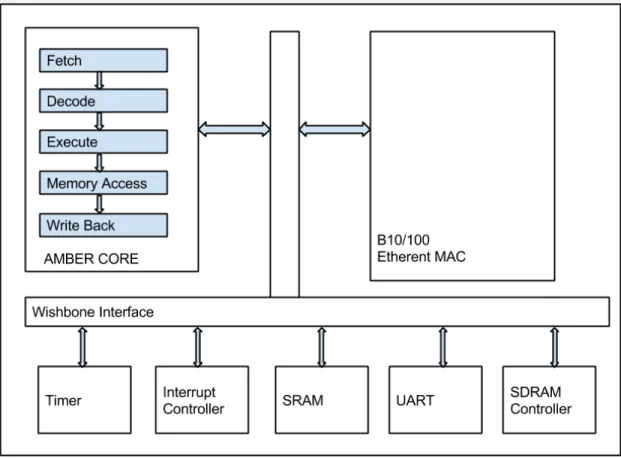
For all experiments in this thesis we used the ARM AMBER core with 5-stage pipeline from Opencores [2]. Figure 1.2 shows all the components of the ARM AMBER System. The whole system has been synthesized to an FPGA and tested for correctness. The core runs at a frequency of 40 MHz without any fault injection. After fault injection we had to reduce the frequency to 30 MHz to avoid timing errors. The processor core consists of the following five stages: Fetch, Decode, Execute, Memory Access and Write Back. Ethernet

(17)

Figure 1.2: ARM ARMBER Architecture

and Amber core are the masters of the wishbone interface, while the slave modules consist of timer, interrupt controller SRAM, UART and SDRAM controller. Further details can be found in the Opencores website

1.3 Restrictions in ARM AMBER

The processor supports ARM v2a ISA and does not have virtual mem-ory. Hence only older linux kernels supporting this architecture can be booted on this FPGA. The current linux version running on the FPGA is 2.4.27. The

(18)

core does not contain a memory management unit and thus does not support dynamic memory management commands like malloc calls. Hence, programs which havemalloc calls had to be hand edited for executing on this machine. The C library used is mini-libc which is also found in Opencores. So programs which used the GNU C library had to be re-written if the specific function library is not found. However, the tools and methods described in this thesis can always be extended to other processor architectures.

(19)

Chapter 2 FPGA Development

Emulation methods remain one of the fastest and most accurate meth-ods for hardware fault injection. The only constraint with FPGA based em-ulation is size of the circuit. Typically we cannot do fault injection on the entire system as this would increase the size beyond the capacity of an FPGA chip or board. So, FPGA based fault injection methods tend to be modular. Civera et al. [17] used a scan chain based strategy for fault injection. Our methodology is similar to theirs in that we also use a scan chain based ap-proach. However, our top-level and software control are different from their methods. Antoni et al. [7] introduced the concept of run time fault injection in reconfigurable hardware. However, this requires extensive support from the FPGA vendor and significant runtime overhead because of circuit reconfigu-ration. More recently PERSIM [10] and Cho et al. [16] implemented FPGA based fault injection system for OR1200 core [3] and LEON3 [1] respectively. The LEON3 fault injection system by Cho et al. uses two copies of the same processor. This is possible as they do fault injection for only 1250 FFs. The core flop count in our case is 3012 and we use a time redundancy approach rather than trying to fit two cores in the same FPGA. PERSIM also uses a two processor approach. However, the golden processor in their case is an ARM

(20)

core that controls the fault injection in the OR1200 core.

The motivation for our FPGA based implementation is manifold. Fast runtime and fine grained control are the foremost reasons. We also wanted to study the effect of soft errors on a more commercial instruction set architecture. This will make the development of multi-level fault injection environment eas-ier. This chapter deals with the development infrastructure for fault injection in ARM AMBER. We used Xilinx’s SPARTAN6 FPGA boards for emulating ARM AMBER system.

2.1 RTL Modifications for Fault Injection

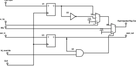
The first step in creating a fault injection environment is to edit the RTL to make it support fault injection. The ARM AMBER core was written in Verilog. Perl scripts were written to automatically modify Verilog for fault injection. The perl script finds each flop in the design and replicates the flop with its copy element along with combinational additions. Figure 4.4 shows the new design. In the figure, U1 denotes the original flop. We replicate this and create the copy element(U3) and stitch the copy elements in a scan chain. The value in the copy flop, along with inj override, decides whether fault is injected on the output of the flop or not. INJ, inv inj, inj override are control signals for fault injection. Inv inj determines whether we need to flip the signal at the output or not. INJ is to inject stuck-at faults in the design. Inj overide is to disable fault injection after a one cycle or specified number of cycles. These control signals are controlled by a system level fault controller.

(21)

Figure 2.1: Modified Flops in ARM CORE

The above structure enables us to insert stuck-at-faults as well as tran-sient bit flips. We select the flop for fault injection based on whether scan in is set to ‘1’ or not for that flop. For the ARM AMBER core there are 3012 FFs in the design. All of them are stitched into a single scan chain. We can choose the number of flip-flops to be bit-flipped by changing the scan sequence. It should be noted that since we are just scanning in the values and then choosing which flops need to be fault injected, there is no need for scan out. The initial versions of FPGA had scan out only for verifying the chain functionality. We can also choose to scan out the flop values to observe the result of corruption as was done by [17] in which they termed it latent fault analysis. However, this cannot be done for large programs.

After successful RTL modifications, the design is synthesized using Xil-inx XST tool. It maps the desgin to Configurable Logic Blocks (CLB) present

(22)

in FPGA. CLBs form the basic programmable unit of FPGAs. Each CLB consists of 4 to 6 inputs, muxes and flip-flops. XST synthesis maps a Verilog based or VHDL based design into CLBs. Synthesis reports of our system show that the register count increased by around 50% and the CLB area increased from 38% to 49%. The muxes used in the modified flip-flop do not cost much because a CLB comes with muxes in it. So, adding two muxes per flop does not significantly increase the size of the design in FPGAs. This is another advantage of using FPGAs for fault injection emulation.

2.2 System-Level Fault Controller

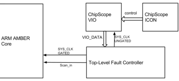
The system level fault controller is responsible for handling the scan sequence. It consists of counters and a state machine for operating the scan. Xilinx Coregen is used to generate Chipscope cores and these are inserted in the design. Chipscope [5] is an embedded software based logic analyzer. We generate and use two cores from Chipscope namely ICON and VIO. The ICON (Integrated Controller) provides communication between VIO and the host computer running ChipScope Analyzer software. The VIO (Virtual In-put/Output) is a core that is used to provide the command for System Level Fault Controller. The System-Level Fault controller also takes care of gat-ing off the system clock when we scan in the sequence. The system clock is activated in the immediate cycle following the bit flip. The processor core ar-chitecture from Chapter 1 can be extended as shown in Figure 2.2. The whole system with peripherals is synthesized and an FPGA bitfile is generated.

(23)

Figure 2.2: ARM AMBER Core with Fault Controller

Fault injection is done on programs which run under Linux. Since operating systems can also crash due to soft-error injection this is a more accurate environment. The linux version used is our setup is version 2.4.27. The limiting factor in these cases is that ARM AMBER does not have virtual-memory management. Hence we had to stick with a basic version of linux. Also, programs had to be edited to change the malloc calls in them.

The steps involved in the fault injection process are as follows. The FPGA is first programmed with the ARM AMBER bitfile, then a Chipscope command is sent from the host PC to initialize the system level fault controller after which linux is booted and then the program is run. For the first run the Chipscope command is a null command with no fault injection. The log is saved for comparison purposes. For the successive runs we send a 64-bit

(24)

command from the Chipscope software to ICON which tells the top-level fault controller the following details.

• Fault-injection type (stuck-at or transient) • Number of scan flops

• Flop ID for injection • Time of fault injection

• Fault Injection Control signals

The Chipscope commands are issued through TCL scripts. For each run the flop ID and injection time are randomly chosen. For larger programs the run times were bigger and so the time to inject faults had a bigger range. To still have a 64 bit command we optimized away the bits denoting injection type and control signals as we are only inserting transient faults in this study. We also hard coded the number of scan flops as they are unique for a design.

2.3 Automation with Pyserial

Each time the processor is programmed in the FPGA, we issue the Chipscope command as explained in the previous paragraph. The next step is to boot linux and load the application. For this we need a serial interface from the host PC. A simple solution for this interface would be minicom (minicom is a linux program commonly used for creating a remote serial console) but

(25)

automating minicom is tedious and since we need to do this several times we used Pyserial [4] which is a Python library for serial port access. The Python program would initialize a serial port connection through USB and load the linux kernel image and the program image via XMODEM (XMODEM is a simple file transfer protocol used in embedded applications). Then the program would initiate the execution of the kernel image.

In summary, every fault injection run involves programming the FPGA, issuing Chipscope commands through TCL scripts, then booting linux and finally, loading and executing the application. The entire process is completely automated so that fault injection can be done several times. With this setup, a minimum of 50,000 fault injections were performed in the FPGA for various applications.

Table 2.1 shows the run times achieved by FPGA based fault-injection at core speed of 30 MHz when compared to simulation times for the same programs. The time taken for the FPGA is 80 seconds because of the overhead of programming the bitfile and booting linux. Running a large program on linux amortizes the cost of booting linux and the total execution time is small, whereas in simulation, execution time increases as the program size increases. Note that the datasets for each of these programs were maintained the same for the simulation and FPGA for comparision purposes. Certain programs can take hours in simulation but would take around the same 80 seconds on the FPGA. The table shows five reference programs among many that were run on the FPGA. AES refers to the program that encrypts and decrypts according to

(26)

Table 2.1: Comparision of Program Run Times

Program FPGA Single run time (sec) Simulation Single run time (sec) CRC 80 88 AES 80 102 Qsort 80 108 Dhrystone 80 952 PID 80 4680

the Advanced Encryption Standard. PID is a Proportional Integral Derivative Controller program. Dhrystone [38] is a common benchmark run on ARM based systems. CRC is the Cyclic Redundancy Checker program. Each of these applications were run 10,000 times in the FPGA. The application is run 10,000 times for statistical fault injection purposes, which are explained in the next chapter. The results of simulation and emulation are also covered in the next chapters.

(27)

Chapter 3 Simulation Based Fault Injection

Simulation based fault injection is a low cost solution to fault injection. A simulation based environment is easier for analysis as it provides fault tracing and cycle accurate waveform dumps for fault injections. VERIFY [36] and MEFISTO-C [19] are VHDL based fault injection simulation environments. The simulation environment developed by Karimi et al. [27] for the IVM processor is similar to ours. However our analysis methods are different from theirs. Our fault injection simulator is built around Xilinx iSim. The simulator has the capabilities of injecting a transient bit flip or stuck at-fault at any cycle and at any point during program execution. Special testbenches were written to test the fault injection environment. These testbenches exercised each case in the fault injection controller. Once the design became stable we were able to simulate assembly programs and C programs. Simulation is too slow for large programs. However simulation provides the best environment for analysis purposes. Propagation paths are easily traceable and internal nodes are also visible in a simulation environment. Hence for an in-depth analysis, simulation is the best method. In order to do both an in-depth analysis as well as fast execution we came up with synthetic benchmarks.

(28)

#include ”amber registers.h” .section .text .globl main main: ldr r0, r0 data ldr r1, r1 data ... ldr r14, r14 data nop ... nop add r0, r11, r8 nop ... nop testpass: str r3, [r6] b testpass

/* Write a non-zero value to this address to generate a Test Passed message */ AdrTestStatus: .word ADR AMBER TEST STATUS

Data: .word 0x12345678 r0 data: .word 0xff666f90 r1 data: .word 0xc3a8efff ...

r14 data: .word 0x5a78006f

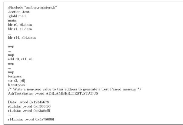
Figure 3.1: A sample benchmark for “add” instruction as the IUT

3.1 Synthetic Benchmarks

Synthetic Benchmarks are a set of small assembly programs designed in such a way that while running these micro benchmarks we would be able to capture the list of most vulnerable flip-flops in the design. Figure 3.1 is an example of a synthetic benchmark for a simple add instruction.

We developed these micro benchmarks for all architectural features of ARM AMBER and simulated them. The architectural features were explored in terms of the instruction set, and each instruction type had its own bench-mark. The data for the instructions are Hamming distance separated so that

(29)

(30)

they are less biased by data changes. Fault injection is done only when the instruction is in the pipeline. For example in the figure 3.1 we inject faults repeatedly during the period where the add instruction is in the pipeline which is why add instruction is surrounded by nop’s. Since the processor has a five stage pipeline, the time we need to do fault injection reduced drastically when compared to large programs. Thus, the main advantage of using synthetic benchmarks is that it takes far less time than running any existing high level benchmark programs like SPEC [23] or MiBench [20].

To validate this claim, we compared the vulnerable flop list obtained from emulating programs on FPGA and the flop list from synthetic bench-marks. We observed that the flop list obtained from synthetic benchmarks is a superset of those flops from FPGA emulation.

3.2 Distributed Statistical Fault Injection Simulation

The synthetic benchmarks that were introduced earlier reduced the problem of when to inject faults. But the design space is still very large and we cannot run synthetic benchmarks for each flop and each cycle between instruction fetch and instruction retirement. This is one of the reasons to turn to Statistical Fault Injection. Statistical Fault Injection [28] applies sam-pling methods to fault injection and gives an upper bound on the number of fault injection experiments that are needed to guarantee completeness statis-tically within a margin of error. We calculated this bound for the synthetic benchmarks and found out that we need to inject around 8000 times for each

(31)

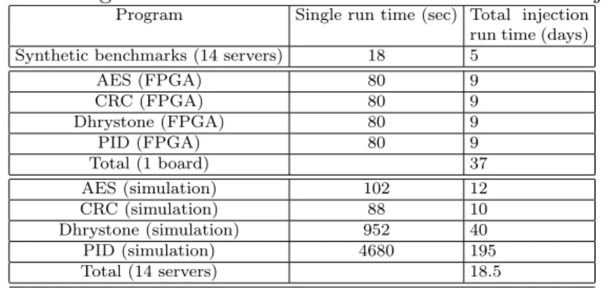
synthetic benchmark at a random point in design space. To learn more about this calculation readers are encouraged to look at our VTS paper [29]. Each fault injection experiment runs the same benchmark for around 8000 times but with the bit-flip on a different random FF in each run. This provides us with an opportunity to make it distributed across different machines. Each run of the synthetic benchmark takes 18 seconds. The total workload was dis-tributed on 14 servers and entire fault injection experiments were completed in 5 days. The distributed fault injection environment was controlled by a perl script on a master machine. The script controlled the load on 14 machines evenly. One important aspect to consider for distributed fault injection is the random number generation. We generated the random number seeds in the master and distributed the seed while scheduling the simulation. We found that if we generate the random numbers in the distributed machines which are running the simulation individually, then the numbers tend to be correlated. In order to avoid this, we generated the random number in the master ma-chine itself. Table 3.1 shows the different run times and compares this with FPGA run-times. It also shows how long a bigger program would take to run in simulation.

Figure 3.3 shows the outcome of running synthetic benchmarks on the processor. Masked failure rates are represented by the blue region. Purple denotes the SDC outcome rates, while timeout and fatal are represented by yellow and black respectively. The SDC rates for push benchmark is higher because this benchmark tests pushing data into memory and any fault injected

(32)

Table 3.1: Program run times on ARM Amber25 for each injection

Program Single run time (sec) Total injection run time (days) Synthetic benchmarks (14 servers) 18 5

AES (FPGA) 80 9 CRC (FPGA) 80 9 Dhrystone (FPGA) 80 9 PID (FPGA) 80 9 Total (1 board) 37 AES (simulation) 102 12 CRC (simulation) 88 10 Dhrystone (simulation) 952 40 PID (simulation) 4680 195 Total (14 servers) 18.5

(33)

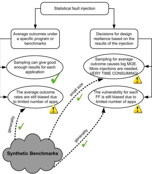
during the execution of this instruction directly affects the output data. From the figure we can infer the rates of SDC, timeout and fatal errors. On average 98.5% of the errors are masked in each benchmark, 0.9% cause SDC, 0.3% cause timeout and 0.3% cause fatal outcomes. This is the reason behind plot-ting Outcome Rates in the figure at 96% rather than 0%. Figure 3.4 shows the single bit and multi bit SDC propagation rates for synthetic benchmarks. These results show that synthetic benchmarks combined with Statistical Fault Injection can become an important part for vulnerability analysis. This is summarized in the Figure 3.2. Figure 3.4 shows that multi bit errors at regis-ters are as equally probable as single bit errors. Hence it shows that inserting single bit errors at register level for soft error analysis is not an accurate model.

(34)

(35)

Chapter 4 Applications of Synthetic Benchmarks

Synthetic Benchmarks discussed in the previous chapter provide inter-esting results for vulnerability analysis. There are several ways to determin-ing the vulnerability of flip-flops. This chapter deals with the vulnerability estimation of flip-flops. Mukherjee et al. [30] came up with the concept of Architectural Vulnerability Factor (AVF) of a design. They estimate AVF of hardware structures like prefetcher, instruction queue, etc. through simulation or manual analysis. This technique can be very manual and does not indicate vulnerability of individual flip-flops. Nair et al. [31] discuss benchmarks that can be used for worst case AVF. This technique is also at the architectural level. The following sections describe other methods for vulnerability estima-tion at flip-flop level.

4.1 Vulnerability Analysis

The vulnerability of a flip flop is given by the vulnerability factor(VF)

V FF Fi =

number of times a sof t error on F Fi causes non−masked outcome number of times a sof t error injected into F Fi

(36)

Figure 4.1: Vulnerability factors of the FFs in ARM Amber25 core which cause erroneous results in synthetic benchmarks

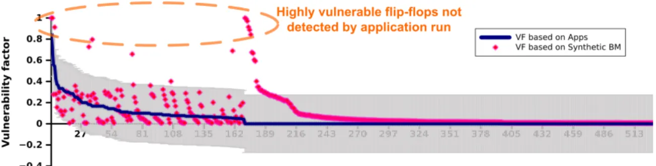
The higher the VF, the more the flop is vulnerable to soft errors. Out of 3012 FFs in the processor core, only 530 of them cause erroneous results in the synthetic benchmarks. Out of these, only 9 FFs have a vulnerability factor of more than 0.8. We cross verified our results with FPGA runs and found that these flops have high vulnerability in those runs too. Studying these flip-flops showed that they have high VF because of their functionality and method of design. Figure 4.1 and 4.2 show the vulnerability factor of flip flops obtained from synthetic benchmarks and applications respectively. Synthetic benchmarks identify flops which are not detected by applications as can be seen from 4.3.

4.2 Data Mining Based Vulnerabilty Estimation

Data Mining and Machine Learning are becoming everyday buzzwords in the research community. This chapter will discuss some of the experiments

(37)

Figure 4.2: VF of ARM Amber25 core FFs which cause erroneous results in four applications. Note the IDs are different from the ones in Fig. 4.1

Figure 4.3: Vulnerability Factors of FF’s from FPGA Applications and Syn-thetic Benchmarks

(38)

that were done for extracting meaningful data from the simulation runs and the FPGA runs. In this chapter we will discuss combining soft error analysis with machine learning techniques. Analytical approaches like the one presented by [9] are better for small designs but as design size grows analytical methods do not scale. The training data for the mining tool is derived from the analytical approaches.

Let us consider the ARM AMBER RTL as a Directed Acyclic Graph (DAG). For every FF in the design, we do a breadth-first search (BFS) and the search ends when we reach the observable elements like register files or output ports of the chip. Then we could rank each level in the graph based on the level order obtained from the breadth-first search. The rank of the level closer to the fault injection node would be higher than the level which is further off the node. The search stops once we reach the output node or registers. A 2-D matrix is created for this with a row for every fault injection node and columns for the number of flip-flops. Let us assume we do fault injection 8K times for a design with 3K flops. Then there would be 8K testcases as rows with 3K flops as columns ranked based on their position in the breadth-first search. This 2-D matrix is the training data for our machine learning models. The results of fault injection form an 1D array which forms the output values for the training data. Suppose the fault causes an SDC; then we mark the corresponding value in the 1-D array as ’1’ and ’0’ if there is no SDC or crash. We can feed the 2-D array with 8K testcases and all 3K flops as attributes and the 1-D array as the result. The next step is running this on decision tree models for this

(39)

data-set. Some of the algorithms we have tried include classification and outlier detection and decision tree learning. Decision tree learning seems to give reasonable results for identifying the key factors involved in fault injection. Pinter et al. [33] have used decision tree learning to identify key factors in dependability experiments of large databases. In our case the decision tree created from the dataset could be used to identify the most vulnerable flops in the design.

Table 4.1: Example Training Set Flop ID A B C X Y Z Y(output corrupted ?)

A 6 5 4 0 0 0 1 B 0 6 5 0 0 0 1 C 0 0 6 0 0 0 1 X 0 0 0 6 5 4 0 Y 0 0 0 0 6 5 0 Z 0 0 0 0 0 6 0

In order to explain how the training set is obtained let us consider a small design with 6 flops, namely, A, B, C, X, Y and Z. A, B and C are connected in a chain with A being the first flop and C being the last flop. Similarly, X, Y and Z are connected in a chain with X being the first flop and Z being the last flop. Both sets of flops are independent and the set X,Y and Z is not connected to any primary output. In this small example the number of test cases is 6, one for each flop. Table 4.1 shows the training set for this small example. Since A, B and C are connected to output or register file the output is always ‘1’ when either A,B or C are affected. However the output is not corrupted if X,Y and Z are fault injected because they are not connected to

(40)

Figure 4.4: Decision Tree with flip-flops

either the output or any register file. Each row corresponds to a fault injection test case. When fault is injected on A, the cell corresponding to A takes the largest number. Since B is connected to A and C is connected B, the breadth first search would rank B next to A and C next to B. Thus the values in the training set are computed. If a decision tree is run on this training set, it will identify A,B and C as the key flops causing output corruption

Figure 4.4 shows the tree obtained for a cache based synthetic bench-mark on our 8k testcases and 3012 FFs. The value of 1 at the bottom of the tree shows that the path ending at ‘1’ is the most vulnerable one pc sel is the program counter select flop which controls the next instruction to be exe-cuted. This is one of the highly vulnerable flops in the design. The presence of dcache wb write data flop in the tree shows that for a synthetic benchmark targeting cache, this flop is one of the most affected nodes. This node is

(41)

not a highly vulnerable node but it becomes vulnerable when load and store instructions are executed. Thus decision trees often give information about nodes which are either easily affected or which are more vulnerable.

4.3 Advantages and Disadvantages

The nodes of the decision tree can give the vulnerable flops in a very clean and automated process. The disadvantage with this method is that the relative absolute error can fluctuate and be high some times. This occurs because the number of instances that fail due to SDC is very low (around 2%). This causes unbalanced class distributions. Our current decision tree algorithm which is J48 in WEKA [21] does not handle unbalanced class distributions. In order to get better accuracy, advanced tree structures like ensembles of α trees [32] need to be used. This is one direction,in which, this research can be extended. As shown in 4.4 decision tree analysis shows some of the most observable nodes in the system. It denotes which of the flops are most vulnerable. We can, in essence, have a good idea of the most vulnerable flip-flops in the design.

(42)

Chapter 5 QEMU Based High Level Error Injection

Software level techniques for evaluating soft-errors are termed error in-jection techniques because we directly inject an error in an architecturally visible component. We consider that the faulty node always causes an error in registers or memory and proceed with this abstraction for software level models. This abstraction in turn leads to lower modelling accuracy as showed by [16]. But the advantages of software models is the execution speed. For running long programs and benchmarks it would be good if we have a software model. Software models gives an instant peek into the dependability of the application. There are various techniques for error injection at the software level. FIAT [35] FERRARI [26] and PROPANE [24] are some of the software implemented error injection tools which are based on injecting error into ar-chitectural components. LLFI [37] and Relyzer [22] are some of the compiler based tools for error injection and error equivalence checking. More recently, Fiesta++ [15] is a more application-friendly error injection environment.

(43)

Figure 5.1: QEMU Based Error Injection Framework

5.1 Error Injection Framework

A similar high level environment for ARM AMBER processor is nec-essary for evaluating high level error models. QEMU [11] is a instruction set simulator which supports v2a ARM instruction set among various others pro-cessor architectures. Figure 5.1 shows the framework of QEMU based error injection. This is quite similar to the framework of other software implemented fault injection methods. All the application programs discussed in the previ-ous chapters were compiled using ARM compilers from Sourcery CodeBench [6] provided by Mentor Graphics. There is also an ARM GDB in this package which we used for our error injection purposes. The Error controller in the figure 5.1 controls the environment. It initiates fault injection by feeding the program to QEMU and also initiates the GDB. The error site and injection

(44)

time are randomly generated by the controller and written to GDB command list. GDB takes care of starting the program in QEMU and inserting the er-ror. The logs are monitored by the error controller and once the injections are done, reports the statistics. The application can be paused at a random time and program location to inject errors in the registers or memory. Each fault injection takes around 3 seconds in a QEMU based environment. A total of 8000 faults takes around 1 hour to complete. This is much faster than either simulation of emulation environments. However, QEMU does not provide as much flexibility as either of the above environments

A high level error model based on our analysis from previous chapter is still in progress. The error injection framework was built to test such a high level environment as single bit errors are highly inaccurate and do not reflect soft errors. A single bit flip in the design can cause multi bit errors in registers as shown in 3.4. These errors can affect either the operand or the operation or the execution of the instruction itself. It can also cause other types of timing errors in the system. It is difficult to accurately model such effects at software level as the parameters we can change in the software are limited.

(45)

Chapter 6 Future Work

There is a lot of scope for improving this research. The synthetic bench-marks can be extended to be more generic and for other processors. The processor used in this work does not have some of the features present in mod-ern processors like out of order execution, virtual memory management and branch prediction. Our current work can be extended to incorporate bench-marks that capture these things. Out of these units, errors affecting branch predictor would not cause any problem. It might increase the latency but correctness will still be preserved. Hence a better and generic framework of synthetic benchmarks is one of the directions to pursue.

Data Mining methods used in this work uses a simple approach. More complex methods can be used to get better results. Mining based techniques are in general more scalable than analytical estimation methods. Hence it is another direction in which this work can be extended

Developing a high level model based on the results of synthetic bench-marks or data mining is another research direction to focus on. A better high level error model will benefit software reliability estimation. Such a high level error model should take into account the probability distribution of single bit

(46)

and double bit errors as well as the distribution of errors in register bits. A generic high level error model is an even ambitious task as error patterns are different across architectures.

(47)

Bibliography

[1] A Gaisler,Leon 3 Processor . http://www.gaisler.com. Accessed: 2015-03-30.

[2] ARM AMBER . http://opencores.org/project,amber. Accessed: 2015-03-30.

[3] OpenRISC . http://opencores.org/or1k/. Accessed: 2015-03-30. [4] Pyserial . http://pyserial.sourceforge.net/index.html. Accessed:

2015-03-30.

[5] Xilinx ChipScope . http://www.xilinx.com/itp/xilinx10/isehelp/

ise_c_process_analyze_design_using_chipscope.htm. Accessed:

2015-03-30.

[6] Xilinx ChipScope . http://www.mentor.com/embedded-software/sourcery-tools/

sourcery-codebench/editions/lite-edition. Accessed: 2015-03-30.

[7] Lörinc Antoni, Régis Leveugle, and Béla Fehér. Using run-time reconfig-uration for fault injection in hardware prototypes. In Defect and Fault Tolerance in VLSI Systems, 2002. DFT 2002. Proceedings. 17th IEEE International Symposium on, pages 245–253. IEEE, 2002.

(48)

[8] Jean Arlat, Yves Crouzet, Johan Karlsson, Peter Folkesson, Emmerich Fuchs, and G¨unther H Leber. Comparison of physical and software-implemented fault injection techniques. IEEE Transactions on Comput-ers, 2003.

[9] Ghazanfar Asadi and Mehdi Baradaran Tahoori. An analytical approach for soft error rate estimation in digital circuits. InCircuits and Systems, 2005. ISCAS 2005. IEEE International Symposium on, pages 2991–2994. IEEE, 2005.

[10] Raghuraman Balasubramanian and Karthikeyan Sankaralingam. Under-standing the impact of gate-level physical reliability effects on whole pro-gram execution. In High Performance Computer Architecture (HPCA), 2014 IEEE 20th International Symposium on, pages 60–71. IEEE, 2014.

[11] Fabrice Bellard. Qemu open source processor emulator. URL: http://www. qemu. org, 2007.

[12] JM Benedetto, PH Eaton, DG Mavis, M Gadlage, and T Turflinger. Dig-ital single event transient trends with technology node scaling. Nuclear Science, IEEE Transactions on, 53(6):3462–3465, 2006.

[13] C Bottoni, M Glorieux, JM Daveau, G Gasiot, F Abouzeid, S Clerc, L Naviner, and P Roche. Heavy ions test result on a 65nm sparc-v8 radiation-hard microprocessor. In Reliability Physics Symposium, 2014 IEEE International, pages 5F–5. IEEE, 2014.

(49)

[14] Th Calin, Michael Nicolaidis, and Raoul Velazco. Upset hardened mem-ory design for submicron cmos technology. IEEE-Transactions-on-Nuclear-Science., pages 2874–8, 1996.

[15] Ameya Suhas Chaudhari. Fiesta++: a software implemented fault injec-tion tool for transient fault injecinjec-tion. PhD thesis, 2014.

[16] Hyungmin Cho, Shahrzad Mirkhani, Chen-Yong Cher, Jacob A Abraham, and Subhasish Mitra. Quantitative evaluation of soft error injection techniques for robust system design. In Design Automation Conference (DAC), 2013 50th ACM/EDAC/IEEE, pages 1–10. IEEE, 2013.

[17] Pierluigi Civera, L Macchiarulo, Maurizio Rebaudengo, M Sonza Reorda, and Massimo Violante. Exploiting circuit emulation for fast hardness evaluation. IEEE Transactions on Nuclear Science, 2001.

[18] Ifeanyi P Egwutuoha, David Levy, Bran Selic, and Shiping Chen. A survey of fault tolerance mechanisms and checkpoint/restart implemen-tations for high performance computing systems. The Journal of Super-computing, 65(3):1302–1326, 2013.

[19] Peter Folkesson, Sven Svensson, and Johan Karlsson. A comparison of simulation based and scan chain implemented fault injection. In Fault-Tolerant Computing, 1998. Digest of Papers. Twenty-Eighth Annual In-ternational Symposium on, pages 284–293. IEEE, 1998.

(50)

[20] Matthew R Guthaus, Jeffrey S Ringenberg, Dan Ernst, Todd M Austin, Trevor Mudge, and Richard B Brown. Mibench: A free, commercially representative embedded benchmark suite. In Workload Characteriza-tion, 2001. WWC-4. 2001 IEEE International Workshop on, pages 3–14. IEEE, 2001.

[21] Mark Hall, Eibe Frank, Geoffrey Holmes, Bernhard Pfahringer, Peter Reutemann, and Ian H Witten. The WEKA data mining software: an update. ACM SIGKDD explorations newsletter, 11(1):10–18, 2009. [22] Siva Kumar Sastry Hari, Sarita V Adve, Helia Naeimi, and Pradeep

Ra-machandran. Relyzer: exploiting application-level fault equivalence to analyze application resiliency to transient faults. In ACM SIGARCH Computer Architecture News, volume 40, pages 123–134. ACM, 2012.

[23] John L Henning. Spec cpu2006 benchmark descriptions. ACM SIGARCH Computer Architecture News, 34(4):1–17, 2006.

[24] Martin Hiller, Arshad Jhumka, and Neeraj Suri. Propane: an envi-ronment for examining the propagation of errors in software. In ACM SIGSOFT Software Engineering Notes, volume 27, pages 81–85. ACM, 2002.

[25] Ravishankar K Iyer, Nithin M Nakka, Zbigniew T Kalbarczyk, and Subha-sish Mitra. Recent advances and new avenues in hardware-level reliability support. Micro, IEEE, 25(6):18–29, 2005.

(51)

[26] Ghani A. Kanawati, Nasser A. Kanawati, and Jacob A. Abraham. Fer-rari: A flexible software-based fault and error injection system. Comput-ers, IEEE Transactions on, 44(2):248–260, 1995.

[27] Naghmeh Karimi, Michail Maniatakos, Abhijit Jas, and Yiorgos Makris. On the correlation between controller faults and instruction-level errors in modern microprocessors. InTest Conference, 2008. ITC 2008. IEEE International, pages 1–10. IEEE, 2008.

[28] R´egis Leveugle, A Calvez, Paolo Maistri, and Pierre Vanhauwaert. Sta-tistical fault injection: quantified error and confidence. In Design, Au-tomation & Test in Europe Conference & Exhibition, 2009.

[29] Shahrzad Mirkhani, Balavinayagam Samynathan, and Jacob A Abraham. In-depth soft error vulnerability analysis using synthetic benchmarks. In VLSI Test Symposium (VTS), 2015 IEEE 33nd, pages 1–6. IEEE, 2015.

[30] Shubhendu S Mukherjee, Christopher Weaver, Joel Emer, Steven K Rein-hardt, and Todd Austin. A systematic methodology to compute the ar-chitectural vulnerability factors for a high-performance microprocessor. In Proceedings of the 36th annual IEEE/ACM International Symposium on Microarchitecture, page 29. IEEE Computer Society, 2003.

[31] Arun A Nair, Lizy Kurian John, and Lieven Eeckhout. Avf stressmark: Towards an automated methodology for bounding the worst-case vul-nerability to soft errors. In Proceedings of IEEE/ACM International Symposium on Microarchitecture, 2010.

(52)

[32] Yubin Park and Joydeep Ghosh. Ensembles of ({alpha})-trees for imbal-anced classification problems. Knowledge and Data Engineering, IEEE Transactions on, 26(1):131–143, 2014.

[33] Gergely Pintér, Henrique Madeira, Marco Vieira, István Majzik, and András Pataricza. A data mining approach to identify key factors in dependability experiments. In Dependable Computing-EDCC 5, pages 263–280. Springer, 2005.

[34] Joydeep Ray, James C Hoe, and Babak Falsafi. Dual use of superscalar datapath for transient-fault detection and recovery. In Proceedings of IEEE/ACM International Symposium on Microarchitecture, 2001.

[35] Zary Segall, D Vrsalovic, D Siewiorek, D Ysskin, J Kownacki, J Barton, R Dancey, A Robinson, and T Lin. Fiat-fault injection based automated testing environment. InFault-Tolerant Computing, 1995, Highlights from Twenty-Five Years., Twenty-Fifth International Symposium on, page 394. IEEE, 1995.

[36] Volkmar Sieh, Oliver Tschache, and Frank Balbach. Verify: Evaluation of reliability using vhdl-models with embedded fault descriptions. In Fault-Tolerant Computing, 1997. FTCS-27. Digest of Papers., Twenty-Seventh Annual International Symposium on, pages 32–36. IEEE, 1997.

[37] Anna Thomas and Karthik Pattabiraman. Llfi: An intermediate code level fault injector for soft computing applications. Silicon Errors in Logic System Effects (SELSE), 2013.

(53)

[38] Reinhold P Weicker. Dhrystone: a synthetic systems programming benchmark. Communications of the ACM, 1984.