Institute
for
International
Economic
Policy
Working
Paper
Series
Elliott
School
of
International
Affairs
The
George
Washington
University
Multidimensional
Poverty
and
Interlocking
Poverty
Traps:
Framework
and
Application
to
Ethiopian
Household
Panel
Data
IIEP
WP
2011
04
Sungil
Kwak
and
Stephen
C.
Smith
Department
of
Economics
and
Institute
for
International
Economic
Policy
George
Washington
University
Washington
DC
20052
June
10,
2011
Institute for International Economic Policy
1957 E St. NW, Suite 502
Voice: (202) 994‐5320
Fax: (202) 994‐5477
Email:
[email protected]
Web:
www.gwu.edu/~iiep
Multidimensional Poverty and Interlocking Poverty Traps: Framework and Application to Ethiopian Household Panel Data
June 10, 2011
Sungil Kwak and Stephen C. Smith∗
Department of Economics,
and Institute for International Economic Policy George Washington University,
Washington DC 20052.
IIEP Working Paper Series 2011-04
∗Send correspondence to [email protected]. We would like to thank Shahe Emran, James Foster, John Hoddinott, Takashi Kurosaki, Travis Lybbert, and participants at the Northeast Universities Development Consortium Conference at MIT (Nov. 2010), and seminars at GWU, Korea Institute for International Economic Policy (KIEP), Korea Institute for Industrial Economics and Trade (KIET), and Samsung Economic Research Institute (SERI) for valuable comments. Research support from the Institute for International Economic Policy at GWU is gratefully acknowledged.
Abstract: This paper examines the impact and potential interactions of health, education and consumption dimensions of persistent poverty at the household level. Our application is to indictors of assets, undernutrition, and illiteracy drawn from the Ethiopia Rural Household Survey (ERHS) panel data set. We develop a framework for operationalizing the concept of multidimensional traps, involving two or more simultaneous distinct poverty dimensions of persistent poverty; these include a subset of cases in which an interlocking poverty trap is effectively formed as a result of deprivations functioning as complements. We test an implication of the multiple trap framework by comparing structural income dynamics across groups. We find that in the poorest of the three main agro-ecological regions in Ethiopia, those with both chronic undernutrition and illiteracy have the lowest implied equilibrium; those with one of these chronic conditions have intermediate (but still deeply poor) equilibria; and those without either condition have the highest asset equilibrium. Evidence for complementarity of persistence across dimensions of poverty - what we term an interlocking poverty trap - is found in only a limited number cases, however. We present several robustness checks for our results.
JEL Classifications: O1, I3
Key Words: Poverty, poverty trap, Ethiopia, multidimensional poverty, interlocking poverty, regional poverty, literacy, undernutrition, asset dynamics
Contents
1 Introduction 1
2 Multidimensional Poverty Traps: Conceptual Framework 2
3 Empirical Literature Review 6
4 Data: The Ethiopia Rural Household Survey 7
5 Asset Dynamics in the Presence of Undernutrition or Illiteracy Trap 12
6 Analysis of Interlocking Poverty Traps 17
7 Concluding Remarks 26
Endnotes 29
References 32
Appendix A 35
A.1 Descriptive Statistics . . . 35 A.2 Land Weight . . . 40
List of Tables
1 Poverty Measures from 1994 to 2004 . . . 9
2 Average Asset Index with Status of Poverty Traps . . . 10
3 Average Education Attainment Years of Sons and Daughters based on Household Illiteracy Trap Status . . . 16
4 Interlocking Poverty Trap Analysis across Regions . . . 18
A-1 Descriptive Statistics . . . 35
A-2 Consumption per Adult and Asset Index across Farming System Regions . . . . 36
A-3 Inequality Measures from 1994 to 2004 . . . 37
A-4 Asset Index with the Status of Undernutrition Traps . . . 38
A-5 Asset Index with the Status of Illiteracy Traps . . . 38
A-6 Asset Index with the Status of Poverty Traps: Robustness Check . . . 39
A-7 Summary of Lands Cultivated: Round 5 . . . 40
A-8 Plot Weight . . . 40
List of Figures
1 Multiple Equilibria . . . 3
2 Single Stable Equilibrium . . . 3
3 Ethiopia Rural Household Survey Villages . . . 8
4 Bayesian Penalized Spline: Comparison between Illiteracy Trap Group and Non-Illiteracy Group across Farming System Regions . . . 14
5 Quantile Regression: the Highlands Area . . . 20
6 Quantile Regression: the Enset Area . . . 21
7 Asset Dynamics across Trap Status: All Areas . . . 24
8 Asset Dynamics across Trap Status in the Enset Area . . . 25
9 Asset Dynamics across Trap Status in the Highlands Area . . . 25
A-1 Asset Index Distributions by Regions for Round 1, 5, and 6 . . . 42
A-2 Illiteracy, Non-illiteracy, and Non-Trap: Full Sample . . . 43
A-3 Undernutrition and Non-undernutrition: Full Sample . . . 44
A-4 Illiteracy Trap: the Enset Area . . . 45
A-5 Undernutrition Trap: the Enset Area . . . 45
A-6 Nonparametric Quantile Regression: Illiteracy trap . . . 46
A-7 Nonparametric Quantile Regression: Undernutrition trap . . . 47
A-8 Quantile Regression: Full samples . . . 48
A-9 Robustness Check: Asset Dynamics in the Enset Area . . . 49
1
Introduction
Conditions of poverty often appear to be the very conditions that make escape from poverty so difficult: challenges posed by such self-reinforcing mechanisms, often called vicious circles, or poverty traps, are an enduring theme of the poverty and development literature. A sub-stantial body of economic theory has demonstrated the essential logic of this possibility. But taken as a whole, empirical findings on whether poverty traps actually exist have been incon-clusive. Recently, the focus of the poverty measurement literature has turned from single to multiple dimensions of poverty (Alkire and Foster, 2011). This paper extends the analysis of one poverty trap to simultaneous potential traps, and introduces an econometric analysis of
multiple dimensions of chronic poverty and potentially interlocking poverty traps.1
In recent years multiple and interlocking poverty traps have been used as a case-study based term for a region, village, or family with two or more distinct poverty problems. Plausibly, the simultaneous presence of different types of poverty traps makes poverty reduction for the extremely poor more difficult. For example, low farm assets, poor nutrition, and illiteracy may each cause income gains to be slow. Moreover, relaxing one of these constraints may result in few gains because another constraint is quickly reached; and then progress on the first problem may even be undermined or reversed. These conditions may reinforce each other; in a well-known framework (Dasgupta, 1993), saving to build assets may be difficult when food is the priority (which we may call a low asset trap), but poor nutrition itself keeps productivity and
hence incomes low (an undernutrition trap).2
Based on insights gained from their direct field experience and other reported case stud-ies, and some evidence on impact, policymakers and practitioners have often implemented approaches to help address poverty which is multidimensional in character, taking into account that some dimensions of poverty may essentially interact so as to reinforce the chronic inci-dence of some or all of the individual dimensions. Among government-sponsored programs, Mexico’s pioneering Opportunidades-Progresa and many subsequent conditional cash transfer programs operate on the assumption that undernutrition, poor-health, low schooling, and child labor are interrelated. The interrelated provision of income support, health, and schooling is a common feature of these programs. A number of well-known NGOs providing microfinance
such as BRAC have integrated provision of credit with health, training, education, and legal
services.3 Grameen, despite sometimes being described as a “minimalist” supplier of credit
alone, has in fact also provided training, and encouraged behavioral change. There is some
evidence that integrated programs can be effective.4 But the econometric literature to date
has not systematically analyzed the incidence of multiple dimensions of poverty that can be mutually reinforcing.
Our approach is to test an implication of the multidimensional trap framework by comparing structural income dynamics across groups. We find that in the poorest of our three regions, those with both chronic undernutrition and illiteracy have the lowest implied equilibrium; those with one of these chronic conditions have intermediate (but still deeply poor) equilibria; and those without either condition have the highest asset equilibrium. Our methods may be useful in other settings to inform program design and policy priorities.
The remainder of the paper is organized as follows. Section 2 covers basic theories of multi-dimensional poverty traps. We examine how multimulti-dimensional poverty traps may be mutually reinforcing given complementarities of inputs in household production functions. An empirical literature review on poverty traps is presented in section 3. In section 4, we introduce the Ethiopia Rural Household Survey (ERHS) and provide descriptive statistics for our main indi-cators of interest. Section 5 examines problems of identifying differences in implied equilibria for all households, combined from all the agro-ecological regions, in either illiteracy or undernu-trition traps. Section 6 utilizes semi- and non-parametric methods to distinguish regional and subgroup cases where no multidimensional poverty is present, where multidimensional poverty is present but these traps do not exhibit complementarity, and where complementarity among poverty traps are present. Furthermore, we investigate the plausibility that two or more traps are mutually reinforcing; we adopt the term “interlocking” poverty traps for this type of inter-action. We conclude in section 7.
2
Multidimensional Poverty Traps: Conceptual Framework
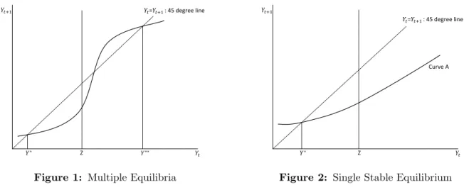
Poverty traps have been studied within consumption and asset space as a vicious circle, or Pareto-dominated equilibrium. Many theoretical contributions have studied thresholds in asset
or capital accumulation that effectively constrain the household from further growth of income as seen in Figure 1. Proposed explanations of thresholds are various: for example, nonlinear-ity in the relationship between nutrition and productivnonlinear-ity (Leibenstein, 1957; Stiglitz, 1976; Dasgupta, 1997), and liquidity constraints faced by households (Loury, 1981; Galor and Zeira, 1993), among others. These explanations are related to incomplete markets and under some conditions generate multiple equilibria so that poverty can be persistent if any shock reduces current income below the unstable equilibrium. A parallel tradition has in effect treated curve A in Figure 2 as a single-equilibrium poverty trap with convergence to a low-level equilibrium
below the poverty lineZ.5
ܻ௧ାଵ ܻ௧ ܻ௧=ܻ௧ାଵ:45degreeline ܻכ Z ܻככ
Figure 1: Multiple Equilibria
ܻ௧ାଵ ܻ௧ ܻ௧=ܻ௧ାଵ:45degreeline Z CurveA ܻכ
Figure 2: Single Stable Equilibrium
The presence of multiple deprivations also appears in basic assets, education and/or health components of the new United Nations Development Programme Multidimensional Poverty Index, that reflects the view that poverty is multidimensional, incorporating multiple aspects. (See Anand and Sen (1997), Alkire and Foster (2011), and UNDP (2010).) In the dual cut-off method, for each household it is first determined whether deprivation in each element is sufficiently severe to be deemed deprived in that element (in UNDP practice this indicator is binary but it could be made continuous with a set threshold such as z-scores as we use in this paper). But only when a sufficient number of deprivations have been counted are individuals in the family deemed multidimensionally poor. This procedure results only in a measure of the existence and extent of poverty. However, it is plausible that severe and chronic deprivation in more than one dimension interacts and increases the difficulty of moving out of poverty across each of the component deprivation. Thus, this paper is complementary to the new research
on multidimensional poverty and contributes to taking a step beyond measuring multidimen-sional poverty to examining its potential effects. These effects are likely to differ depending on the type and severity of the deprivations and the degree to which they interact (or act as complements in keeping individuals trapped in poverty).
Moving from concepts of poverty measurement to an examination of conditions under which some forms of poverty traps may emerge, we start with the observation that, potentially, char-acteristics of asset equilibria differ across regions and across types of deprivations. Moreover, an economy that behaves with the properties of a local trap given current conditions may not behave similarly after conditions change (such as a sufficient increase in average national income raising demand, or newly available farming technologies). In this regard, observing poverty traps in more than one asset or welfare indicators in one region may predict more poverty persistence than in another region with just one deprivation, when other conditions in the wider economy improve. Moreover, an estimated equilibrium above the poverty line for a given region may effectively assume that complementary factors are correspondingly increased, but in the presence of other constraints the poor may be prevented from acquiring the needed achievements, such as acquiring requisite complementary skills.
With these motivations, we proceed to expand the one dimensional model of income dynam-ics to a multidimensional model. Defining household assets broadly to include human capital and other resources, the following is the system of household asset growth functions.
Yit R1it R2it .. . Rmit = f(Yit−1, R1it−1, R2it−1, ..., Rmit−1, Xit) g1(Yit−1, R1it−1, R2it−1, ..., Rmit−1, Xit) g2(Yit−1, R1it−1, R2it−1, ..., Rmit−1, Xit) .. . gm(Yit−1, R1it−1, R2it−1, ..., Rmit−1, Xit) , (1)
where Yit is the household current income, Rjit is amount level of current resources, j =
1,2, ..., m, of each household, i = 1,2, ..., n. Resources and household income level at t−1
determine both current income level (Yit) and current level of each resource (Rjit). Xitincludes
the households are more likely to be trapped in income and resources, since the households cannot save sufficiently to invest for future resources. As a result, there are inadequate resources
to increase nutrition, education, and so on. Hence, m + 1 dimensional poverty traps could
appear. If two or more traps are present simultaneously, we term this a multidimensional poverty trap. If they are also mutually reinforcing through complementarity, we term them “interlocking” poverty traps. This method can help determine the larger or smaller sets of combinations of deprivations that have a large functional impact on poverty persistence and severity in a given region.
The presence of multiple human capital deprivations may function as a self-reinforcing mechanism which causes low human capital accumulation – “and hence poverty –” to persist. Under-nutrition (or very low health capital generally) may lower the return on investment in education: for example, under-nutrition reduces school attendance; and undernourished chil-dren perform poorly even if they are able to attend school; and undernourished individuals are less able to productively use education at any point in life. On the other hand, public health and nutrition programs are likely to be unsuccessful when intended beneficiaries are illiterate, and lack of schooling means children are not taught basic personal nutritional guidelines, hy-giene, and sanitation. Chronic deprivation of one form of human capital therefore can lead to disincentives to invest in other forms of human capital; and this problem can be decisive at very low levels of consumption when any saving is challenging. Note that we are describing individual investment incentives and constraints - even before considering complementarities across individuals that could compound the difficulties. Moreover, the combination of human capital deprivations may reduce the potential benefits of other forms of asset accumulation, even if some savings resources were available.
Our empirical approach allows for the possibility that lack of one type of asset or capability can be made up for (substituted) by other assets - but only to a degree, as a sufficiently large set of missing assets together function as complementary inputs. For example, health and education to a degree might act as substitutes for each other in allowing the accumulation of assets, but when both are lacking this may prevent accumulation. For the very poor, the lack of a resource such as health or education can through strong complementarity change the household asset growth function. This reflects that the very poor are more likely to own few
resources that can function as substitutes after some point. In the extreme, lack of one resource even prevents the resources that the poor household have from providing more than negligible productivity.
In this paper, then, we also investigate the existence of interlocking poverty traps by explor-ing the existence of such complementarities. In the range of extreme poverty, household assets such as health, nutrition, education, and farm capital, may function as strong complements in equation (1).
3
Empirical Literature Review
Empirical research into multiple equilibria even with a single indicator of interest has begun fairly recently (Jalan and Ravallion, 2001, 2002; Dercon, 2004; Lokshin and Ravallion, 2004; Lybbert et al., 2004; Adato et al., 2006; Barrett et al., 2006; Naschold, 2009; Campenhout and Dercon, 2009). Both parametric and semi/nonparametric estimation methods have been used to estimate poverty dynamics but almost exclusively only in either income or asset space. However, poverty traps could appear in other dimensions. Hoff and Stiglitz (2001) point out that ‘low-level equilibrium traps’ can occur due to lack of other indicators of welfare (for example, lack of political freedom or institutions).
Just a few studies have investigated whether a single dimensional poverty trap exists in other dimensions beyond income and assets.
For example, Emerson and Souza (2003) present empirical evidence on the intergenerational persistence of child labor using the 1996 Brazilian Household Survey. They find that parental child labor significantly increases the probability that their child will work in the labor market, and that the more years that parents worked as children, the greater their own children’s likelihood of entering the labor force. In addition, they find that past child labor significantly reduces current income (which increases the incentive, or the necessity, for child labor also from the following generation).
Mayer-Foulkes (2008) presents existence of a human capital accumulation trap in Mexico using the 2000 National Health Survey (ENSA 2000); he finds that schooling is an important factor for adult income; that the schooling experience of parents significantly affects the
school-ing decision of adolescents; and that the shapes of schoolschool-ing year distributions over time have double-peaks. He proposes that the composition of all three findings support the existence of multiple equilibria in human capital space.
Jha et al. (2009) use the data from the National Council for Applied Economic Research (NCAER) and test for the existence of an undernutrition trap in rural India. They focus on agro-climatic zones to acquire homogeneity (i.e. agricultural activity). Using Heckman’s (1976) sample selection model, they estimate the impact of micronutrient consumption on wage rates over various categories of work, and find some evidence of undernutrition traps.
As proposed in section 2, however, the extremely poor could have two or more poverty traps simultaneously, which can interact complementarily to hinder the accumulation of house-hold assets. Therefore, we introduce idea of multidimensional poverty traps to this literature, including the examination of complementarity across traps, which we call interlocking traps.
4
Data: The Ethiopia Rural Household Survey
This study uses Ethiopia Rural Household Survey (ERHS) data set6: First, per capita income
in Ethiopia is one of the lowest in the world7; yet, rural Ethiopia has experienced “pro poor”
growth.8 We have opportunities to examine conditions under which the poor might be escaping
from poverty traps. ERHS contains information that can be used to explore multiple traps beyond income and assets, including basic health and basic education. These might help us understand why some families and regions might fail to benefit even in a general national environment of pro poor growth.
ERHS is publicly available by International Food Policy Research Institute (IFPRI). ERHS
studies 1,477 households residing 15 villages, stratified in three agro-ecological zones of Ethiopia.9
Households are randomly selected within each village. In the data, population shares are broadly consistent with the population shares in the three main sedentary farming systems, which are the grain-plow complex highlands, the grain-plow/hoe complex, and the enset growing area. Figure 3 represents the survey sites and 3 categories according to farming systems in rural Ethiopia.10
Geblen Haresaw Shumsha Yetmen DebreBerhan AdeleKeke Korodegaga SirbanaGodeti Imdibir AzeDeboa Doma Adado TurfeKechemane Dinki GaraGodo
GrainͲPlow/hoeComplex
GrainͲPlowComplexHighlands
EnsetGrowingArea
Figure 3: Ethiopia Rural Household Survey Villages
of land is a key to economic activity in Ethiopia. Thus, when households migrate to another region, they have a difficulty in acquiring land from an unfamiliar peasant association. Naturally mobility is highly restricted. Moreover, due to insecure land holding system farmers do not have an incentive to invest in lands. Thus, farmers have low productivity from land and perpetuating
low growth. At the end they stay in poverty.11
We first investigate changes in poverty from 1994 to 2004 over the 3 agro-ecological regions.
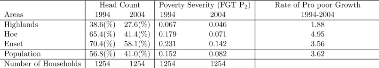
Table 1 presents the 1994 and 2004 poverty measure for the ERHS sample of 1,254 households.12
Comparing the 1994 measures with the measures in 2004, we find that the expenditure based poverty measures decreased. The head count measure decreased from 56.8% to 41.0%. In addition, the FGT poverty severity measure decreases from 0.152 to 0.082 over time. Comparing the poverty measures across the 3 regions, we find that the enset area has the largest population suffering from poverty. The basic head count measure of the enset area is almost twice that of the highlands area in both 1994 and 2004. Even though rural Ethiopia experienced the pro poor growth, Table 1 suggests that the poor in the enset area have tended to stay poor. That is, the poor fail to escape from poverty over time even with pro poor growth.
To date, the econometric literature on poverty traps has focused on the presence of one di-mensional trap, indexed by a single variable, generally an asset index or consumption. Barrett et al. (2006) present that current income and consumption is not sufficient to identify chronic poverty since this flow includes both structural and stochastic components of income
simultane-Table 1: Poverty Measures from 1994 to 2004
Head Count Poverty Severity (FGT P2) Rate of Pro poor Growth
Areas 1994 2004 1994 2004 1994-2004 Highlands 38.6(%) 27.6(%) 0.067 0.046 1.88 Hoe 65.4(%) 41.4(%) 0.179 0.071 4.95 Enset 70.4(%) 58.1(%) 0.231 0.142 3.56 Population 56.8(%) 41.0(%) 0.152 0.082 3.62 Number of Households 1254 1254 1254 1254
aPoverty lines are set by real consumption of 72 Birr per adult equivalent per month, which is equivalent to $1 per day in 1994. bRate of pro poor growth is the mean of growth rate at each percentile of the expenditure distribution up to the headcount poverty
measure. The numbers are estimated, following Ravallion and Chen (2003). The numbers measure how much the poor is benefiting from growth.
cThe poverty severity measure, 1 N
�M i=1(
z−yi z )
2, was developed and axiomatically justified by Foster et al. (1984).
ously. Using the structural part of income, (i.e. assets), has an advantage for analyzing chronic poverty and poverty traps. Therefore, we estimate an asset index, which provides a proxy for
household structural income.13
For present purposes, we have defined an illiteracy trap as remaining illiterate throughout
the five periods.14 In addition, we construct an undernutrition trap variable using
anthropo-metric data.15 After comparing the indicators, we adapt the z-scores of BMI-for-age from the
widely used 1990 British Growth Charts to generate an undernutrition trap status variable.16
The z-score of BMI-for-age is represented as
z-score(BMI/Age)= BMIijk−Median BMI
reference population
jk
S.D.reference populationjk , (2)
where BMIijk represents the BMI of an individual i, i = 1,2, ..., n whose age is k and whose
gender(male/female) isj. We define a household as trapped if any members have BMI-for-age
z-scores<-2 throughout the sample.17 Using this simple definition, we find that 17.9% of the
full sample are trapped.18
Based on poverty trap status, we examined whether households have different patterns of structural income levels. We use a simple t-test and the Epps-Singleton test for whether both trapped groups have the same mean and the same distribution, respectively. (See Tables A-4 and A-5 in the Appendix for detailed estimates.) We find that in the highlands area a house-hold in an illiteracy trap does not have lower structural income (p-value is 0.7921) than those not trapped, while structural incomes in the other areas differ significantly depending on trap status. The difference of average asset index in the highlands area is 0.05, while other areas has
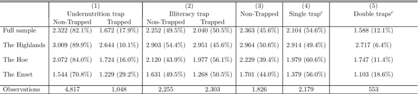
Table 2: Average Asset Index with Status of Poverty Traps
(1) (2) (3) (4) (5)
Undernutrition trap Illiteracy trap Non-Trapped Single trapc Double trapsc
Non-Trapped Trapped Non-Trapped Trapped
Full sample 2.322 (82.1%) 1.672 (17.9%) 2.252 (49.5%) 2.040 (50.5%) 2.363 (45.6%) 2.104 (54.6%) 1.588 (12.1%)
The Highlands 3.009 (89.9%) 2.644 (10.1%) 2.903 (54.4%) 2.951 (45.6%) 2.964 (50.6%) 2.914 (49.4%) 2.717 (6.4%)
The Hoe 2.072 (84.0%) 1.724 (16.0%) 2.120 (43.9%) 1.977 (56.1%) 2.229 (39.4%) 1.979 (60.6%) 1.747 (11.4%)
The Enset 1.544 (70.8%) 1.229 (29.2%) 1.631 (49.5%) 1.268 (50.5%) 1.701 (44.0%) 1.379 (56.0%) 1.103 (18.6%)
Observations 4,817 1,048 2,255 2,303 1,826 2,179 553
aThe proportion of the households having each trap status is in parenthesis.
bWe only use the observations that we can identify both undernutrition and illiteracy trap status to define a single trap and double trap
(n=4,558). The reason is that if we know the information of only a single trap, the trapped households may have another trap that we fail to identify. Hence, we only use the cases that both trap status are identified. As a robustness check, we include all the cases that we fail to identify either illiteracy or undernutrition trap in Table A-6.
cSingle trapped households in the fourth column represent the households that have only one trap regardless of undernutrition and illiteracy.
Double trapped households have both illiteracy and undernutrition trap simultaneously.
larger difference: 0.15 and 0.37 for the hoe and the enset areas, respectively. We note, however, that the distribution of structural income in the highlands area varies significantly depending on illiteracy trap status at any conventional level. Moreover, a household in an undernutrition trap has lower structural income regardless of the region. In addition, we find that the distribu-tions of the trapped and non-trapped household incomes are significantly different within each region, and across the traps. Moreover, we find that the illiteracy and undernutrition traps are significantly positively correlated.19
Table 2 shows the average structural income according to trap status. Trapped households have lower structural income levels than non-trapped households. In particular, comparing the difference of the average structural income between the illiteracy trapped group and the non-illiteracy trapped group across regions, we find that the difference is largest in the enset area; the difference is the smallest in the highland area. These findings suggest that an illiteracy trap affects the asset level heterogeneously over the income (or regional) distribution. In contrast, comparing the difference of the average structural income between the undernutrition trapped group and the non-undernutrition trapped group across regions, we find that the difference is around 0.35 over the three regions. This implies that an undernutrition trap affects the asset level uniformly.
In addition, comparing the proportion of trapped households within each region, we find that the highlands area has the smallest proportion in each trap. The enset growing area has
households may have an incentive to invest more in education if access to and accumulation of other assets is difficult, the smaller differences in the proportion of households in an illiteracy trap across regions can be explained. Households in the most deprived area may have more incentive to invest in education if the rate of return on schooling is high under the assump-tion that assets are substitutes. Therefore, the illiteracy trapped households seem to have a somewhat different set of characteristics from those in an undernutrition trap.
The column (3) provides the average asset index level of non-trapped households. The highlands area has the highest asset holding level, while the enset area records the lowest level. The column (4) in Table 2 represents the average structural income (asset index) of households with a single trap, regardless of what kind of traps households have. First, note that the difference between asset levels of single-trapped (column (4)) and non-trapped (column (5)) households in the full sample (that is, treating regions as homogeneous) is small, about 10.96%. Comparing the asset level of double trapped households in column (5) with non-trapped households in column (3), however, the gap is triple (32.80%) that of the difference between the non-trap and single trap. This finding may support our argument in section 2; when one resource is missing in the household asset accumulation function, other resources can make up for it. When both resources are missing simultaneously, however, trapped households could be prevented from household asset accumulation by complementarity of resources since the very poor are more likely to have only a small amount of other resources.
As we have already, however, poverty conditions differ across the three agro-ecological re-gions. Considering the regional levels, the difference of the average asset index between column (3) and (4) is negligible in the richest area, the highlands area. (t-test statistics= 0.8227, p-value=0.4108 for a two-sided test.) However, the more deprived the area is, the larger the difference is. The enset area, the most deprived area, has the largest difference of asset levels. This finding is more obvious in the case of double trapped households, as seen in column (5). Therefore, this finding provides a hint that the very poor and/or the very poor regions have a higher likelihood that the complementarity of inputs appears in household asset accumulation.
5
Asset Dynamics in the Presence of Undernutrition or
Illiter-acy Trap
We first consider asset dynamics of the full sample treating all regions as homogeneous according to trap status; then we explore further the dynamics of the three regions, according to trap sta-tus, using penalized splines with Bayesian inference proposed by Krivobokova et al. (2009). We first consider asset dynamics of the full sample treating all regions as homogeneous according to trap status; we then explore further the dynamics of the three regions, according to trap status, using penalized splines with Bayesian inference as proposed by Krivobokova et al. (2009). Our indicators for an illiteracy trap and an undernutrition trap are both binary variables, so we can-not estimate the dynamics of these indicators. Instead, we estimate asset dynamics conditional on the illiteracy-trapped and/or undernutrition-trapped status of the households. Compar-ing the asset dynamics given these traps, we gain insight into how these deprivations impact the household asset growth functions (in equation (1)) which in turn would affect other long-term household outcomes. For example, if other household inputs do not sufficiently substitute for literacy deprivations in the household asset growth functions, long-term asset dynamics of illiteracy-trapped households should converge to a statistically lower implied equilibrium than that of non-illiteracy trapped households. The same may be true for undernutrition-trapped households; and when illiteracy and undernutrtion are present simultaneously their combined effects may be more than additive. Figure A-2(a) represents the asset dynamics of illiteracy trapped and non-illiteracy trapped households. Intriguingly, both dynamics converge to the same equilibrium statistically regardless of trap status. The dynamics of undernutrition trap in Figure A-3(a) also converge to statistically the same equilibrium regardless of trap status. In these data, when we combine households from all the agro-ecological regions, we do not identify
differences in implied equilibria for those in either illiteracy or undernutrition (single) traps.21
We examine three hypothetical explanations of these findings: First, neither trap status de-termines the asset dynamics of rural Ethiopia; second, the non-illiteracy (Non-undernutrition) trapped households are also severely affected by undernutrition (illiteracy) traps; third, the household conditions in the three regions are so different that pooling them in this analysis could be misleading.
If the dynamic path of households having no trap is located above the dynamic path of non-illiteracy or non-undernutrition households, we may conclude that other types of trap hinder (or constraints more generally) households from accumulating assets and the trap status determines the asset dynamics. The implied equilibrium of the non-trapped households should be greater than that of the trapped households. On the contrary, if the dynamic path of households having no trap is similar to the dynamic path of illiteracy or undernutrition trapped households; and if both paths converge to the same equilibrium; we conclude that the each trap does not have effect on the asset dynamics on average.
To test these alternative hypotheses, we estimate the asset dynamics of the households hav-ing no trap. From the full sample (that is, treathav-ing regions as homogeneous), we find that the
dynamics overlap and converge to statistically the same equilibrium.22 Hence, we conclude that
the one dimensional traps (i.e., either illiteracy or undernutrition trap), on average, may not determine the long run asst dynamics. However, the traditional mean regression approaches, in-cluding both parametric and nonparametric regressions, may be misleading because the analysis does not fully represent the lower tail of income distribution.
Hence, we next consider the asset dynamics of the three regions according to illiteracy trap
status since the three regions have different income distributions.23 We find that the enset
area is poorest and the highlands area is richest among the three regions in our data set. Figure 4 presents the equilibria of the illiteracy trap group and the non-illiteracy group across farming system regions, respectively. Across all regions, the equilibrium of the illiteracy and non-illiteracy trap group are not significantly different. When households are merged in the data set across regions, they show some differences in structural income on average depending on the trap status as in Table 2. However, they converge to the statistically same equilibrium of structural income in the long run, regardless of trap status in the highlands and the hoe areas. Moreover, the dynamic paths of the highlands and the hoe areas are almost identical regardless of the trap status. However, the dynamic paths in the enset growing area represent different patterns depending on the trap status when we compare them with those in other regions: First, the equilibrium is much lower than in two other regions; furthermore, the dynamic path of non-illiteracy group is located above that of illiteracy trap group.
(a) Highlands Area (b) Hoe Area
(c) Enset Area
Figure 4: Bayesian Penalized Spline: Comparison between Illiteracy Trap Group and Non-Illiteracy Group across Farming System Regions
separately illiteracy and undernutrition traps in the enset area. We find the same patterns of the dynamics as in Figure 4(c). (That is, we compare with the asset dynamics of households having no traps; for details see Figure A-4(a) and A-5(a); Figure A-4(b) and A-5(b) represent the dynamics of households residing in the enset area who suffer from the illiteracy trap and the undernutrition trap, respectively.) We also find that the dynamic paths of households having no trap are located above the paths of both the illiteracy and the non-illiteracy trapped groups, though the difference is not statistically significant. These findings provide at least suggestive evidence that the poverty trap status determines the asset dynamics in the most deprived area.24
In addition, it is still questionable that each asset dynamics converges to the same equilib-rium regardless of trap status in the full sample (that is, treating regions as homogeneous), since the the dynamics at the lower extreme percentile of income distribution are apparently differ-ent from that of median or higher percdiffer-entile of income distribution. To address this important concern systematically, it is insightful to utilize a nonparametric quantile regression known as the quantile smoothing spline. We estimate the relationship, lnyi,t −lnyi,0 = m(lnyi,0) +ei,
using the full sample.25 That is, we estimate the unconditional growth regression for each trap
status. We use the B-spline regression quantiles proposed by Ng and Maechler (2007). The
smoothing parameterλis selected by minimizing the Schwarz information criterion.26
Illiteracy trap status affects the dynamics of the structural income. (For details see Figure A-6 in the Appendix.) We find evidence of poverty traps in the dynamics of both non-illiteracy and illiteracy trapped households from the 20th percentile quantile regression. Excepting the 20th percentile quantile regression, all dynamics from other percentiles have a single stable equilibrium. Interestingly, the dynamics of the illiteracy trapped households converge to a lower equilibrium than that of the non-illiteracy trapped households up to 40th percentile quantile regressions. In above median quantile regressions, however, the dynamics from each quantile regressions have statistically the same equilibrium regardless of the trap status. These findings suggest that the illiteracy trap status is only correlated with the long term dynamics of the households in lower percentiles of the income distribution, not those in higher percentiles. In order to further test this finding, we compute the average education years of both sons and daughters according to the illiteracy trap status of the households, as seen in Table 3.
Table 3: Average Education Attainment Years of Sons and Daughters based on Household Illiteracy Trap Status
Asset Index Nonilliteracy Trapped Illiteracy Trapped t-value Two-sided Test One-sided Test Percentiles Household Household Pr(|T|>|t|) Pr(T > t)
Below 60th percentiles 5.911 4.246 1.955 0.052 0.026
Above 60th percentiles 4.085 4.045 0.042 0.967 0.484
Total 5.031 4.176 1.338 0.182 0.091
aSource: ERHS 1994a.
bThe numbers are average education years of sons and daughters within a household according to the illiteracy trap status of
the household.
cThe alternative hypothesis of the one-sided test is that the education years of children in a non-illiteracy trapped household
are greater than that in the counterpart.
d60th percentiles of asset index is used to identify poor households since we identifies about 60% of households as the poor
households in Table 1.
eEducation years of children are computed by following: aggregating education years of both sons and daughters greater than
13 years old, and then the aggregated number is divided by the total number of the sons and daughters.
As Table 3 reveals, the average educational attainment year of sons and daughters born into non-illiteracy trapped households is significantly greater than the counterparts within house-holds having relatively low asset levels (below 60th percentile of the asset index distribution). However, we fail to find evidence of differences in sons and daughters’ educational attainment between the two groups within households above the 60th percentile of the asset index distri-bution. These findings suggest that the lowest (permanent) income households (as identified by asset levels) can have differing long-term outcomes, such as the human capital level of de-scendants, according to the illiteracy trap status of the current generation. Hence, the long term asset dynamics of future generations within relatively asset poor households may also depend on the illiteracy trap status of the current generation; this could be an explanation of heterogeneous asset dynamics in Figure A-6 in the Appendix. In other words, such households with sufficient assets and consumption may be able to send their children to school and escape intergenerational poverty traps in the longer-run.
The nonparametric quantile smoothing splines of both undernutrition and nonundernutri-tion trapped groups are presented in Figure A-7 in the Appendix: the asset dynamics of both undernutrition and nonundernutrition trapped groups along the structural income distribution. All dynamics converge to the same single stable equilibrium regardless of the trap status, which
is consistent with the mean regression estimation results.27 A plausible explanation of this
result for households suffering from an undernutrition trap is “asset smoothing.” For example, the short term response of undernutrition trapped households is not to sell an animal to buy food, instead they eat less, if they expect that assets’ future rate of returns is greater than
their current rate of returns. In the long run, there is no difference between the dynamics of the trapped households and those of the non-trapped households, since the trapped households
still have their own assets to utilize in the future.28
The Ethiopian evidence examined here suggests a wider implication that in general it will be important for practitioners and policymakers to determine the types of poverty traps (if any) that affect households located in the lower quantiles of the income distribution, since the structural income dynamics of households must evolve in the long run according to which trap is prominent.
6
Analysis of Interlocking Poverty Traps
Thus far we have presented long term evidence that undernutrition and illiteracy traps de-crease households’ asset holding levels in the most deprived region and in households in the lower percentiles of the income distribution. In equation (1), we present that a deprived input in household asset growth functions determines long-term household outcomes with other house-hold resources. We now investigate further whether illiteracy and undernutrition traps work together through complementarity to worsen asset poverty. For example, either undernutrition or illiteracy may impair the ability of the household to accumulate assets, but when both are present their combined or interaction effects may be more than additive.
Since only households that remain in illiteracy (or undernourishment) in all periods are defined as trapped, we cannot simply transform the data to remove the household specific
effect. Hence, utilizing the Mundlak device within the random effect model,29 we construct
a pseudo-fixed effect model. (Mundlak, 1978) This estimation approach allows us to analyze whether or not the illiteracy trap status significantly interacts with the undernutrition trap to worsen asset conditions in the short term, controlling for unobservable heterogeneity. To test this, we include an interaction term between an undernutrition and an illiteracy indicator within our equation (3) estimated.
lnAi =β0+β1P1i+β2P2i+β3P1iP2i+Xiα+ ¯Xiθ+ei, i= 1,2, ..., n, (3)
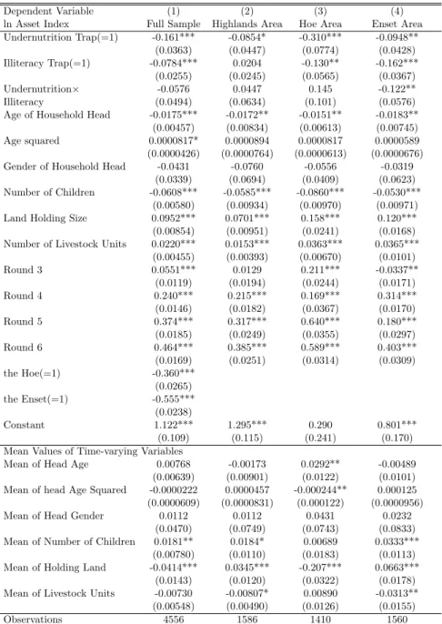
Table 4: Interlocking Poverty Trap Analysis across Regions
Dependent Variable (1) (2) (3) (4)
ln Asset Index Full Sample Highlands Area Hoe Area Enset Area Undernutrition Trap(=1) -0.161*** -0.0854* -0.310*** -0.0948** (0.0363) (0.0447) (0.0774) (0.0428) Illiteracy Trap(=1) -0.0784*** 0.0204 -0.130** -0.162*** (0.0255) (0.0245) (0.0565) (0.0367) Undernutrition× -0.0576 0.0447 0.145 -0.122** Illiteracy (0.0494) (0.0634) (0.101) (0.0576) Age of Household Head -0.0175*** -0.0172** -0.0151** -0.0183**
(0.00457) (0.00834) (0.00613) (0.00745) Age squared 0.0000817* 0.0000894 0.0000817 0.0000589 (0.0000426) (0.0000764) (0.0000613) (0.0000676) Gender of Household Head -0.0431 -0.0760 -0.0556 -0.0319
(0.0339) (0.0694) (0.0409) (0.0623) Number of Children -0.0608*** -0.0585*** -0.0860*** -0.0530***
(0.00580) (0.00934) (0.00970) (0.00971) Land Holding Size 0.0952*** 0.0701*** 0.158*** 0.120*** (0.00854) (0.00951) (0.0241) (0.0168) Number of Livestock Units 0.0220*** 0.0153*** 0.0363*** 0.0365***
(0.00455) (0.00393) (0.00670) (0.0101) Round 3 0.0551*** 0.0129 0.211*** -0.0337** (0.0119) (0.0194) (0.0244) (0.0171) Round 4 0.240*** 0.215*** 0.169*** 0.314*** (0.0146) (0.0182) (0.0367) (0.0170) Round 5 0.374*** 0.317*** 0.640*** 0.180*** (0.0185) (0.0249) (0.0355) (0.0297) Round 6 0.464*** 0.385*** 0.589*** 0.403*** (0.0169) (0.0251) (0.0314) (0.0309) the Hoe(=1) -0.360*** (0.0265) the Enset(=1) -0.555*** (0.0238) Constant 1.122*** 1.295*** 0.290 0.801*** (0.109) (0.115) (0.241) (0.170) Mean Values of Time-varying Variables
Mean of Head Age 0.00768 -0.00173 0.0292** -0.00489 (0.00639) (0.00901) (0.0122) (0.0101) Mean of head Age Squared -0.0000222 0.0000457 -0.000244** 0.000125 (0.0000609) (0.0000831) (0.000122) (0.0000956) Mean of Head Gender 0.0112 0.0112 0.0431 0.0232
(0.0470) (0.0749) (0.0743) (0.0833) Mean of Number of Children 0.0181** 0.0184* 0.00689 0.0333***
(0.00780) (0.0110) (0.0183) (0.0113) Mean of Holding Land -0.0414*** 0.0345*** -0.207*** 0.0663***
(0.0143) (0.0120) (0.0322) (0.0178) Mean of Livestock Units -0.00730 -0.00807* 0.00890 -0.0313**
(0.00548) (0.00490) (0.0126) (0.0155)
Observations 4556 1586 1410 1560
aStandard errors are in parentheses.
bWe use 5 rounds of ERHS. (1994a, 1995, 1997, 1999, 2004) We also use 3 rounds of ERHS (1994a, 1999, and 2004) as a robustness check. The significance of variables do not change.
c∗p <0.10,∗∗p <0.05,∗∗∗p <0.01
illiteracy trap status and undernutrition trap status, respectively, andXirepresent time-varying explanatory variables including age of household head, squared age of household head, gender of household head, number of children, land holding size, and number of tropical livestock units. We also include time dummies to control for the time specific effect. The first column in Table 4 includes regional fixed effect dummies. In column (2) to (4), we estimate equation (3) across farming system regions to explore whether or not both the illiteracy trap and the undernutrition trap negatively affect household structural income level, and whether the traps interact to lower the asset level significantly.
Table 4 provides the estimates from pseudo-fixed effect estimations. The appropriate F-test for the fixed effect model, in which the null hypothesis is that all coefficients of group mean
values are equal to zero, (that is,θ=0) is rejected at any conventional level.30 With specification
(1), the interlocking poverty trap status does not have a significant effect on the percentage change in structural income, while undernutrition and illiteracy traps affect it significantly
at any conventional level.31 From specifications (2) through (4), the significantly negative
coefficient of the interaction term at 5% level in the enset area implies that the simultaneous presence of traps effectively reduces household structural income, that is, significantly reinforce each other, while the coefficients from the highlands and the hoe regions do not. These findings support that the chronic poverty conditions are working together to reduce household structural income level particularly in the most deprived area.
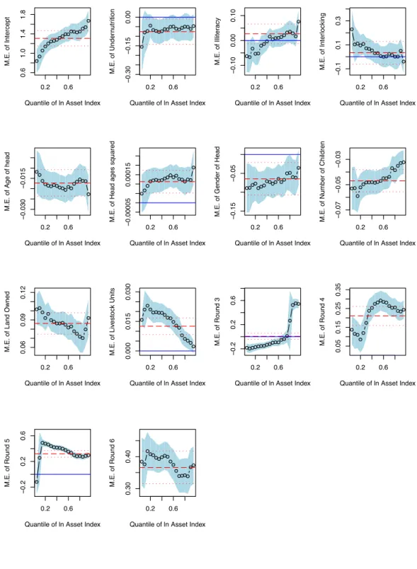
Depending on current asset holding levels of households, the short term relationship of each trap indicator and current asset levels can differ significantly. Among other things very low-asset households may be more likely affected by interlocking poverty traps. We estimate quantile regressions over the structural income distributions in each agro-ecological region using pooled data. Conditional mean regression is (as the name suggest) evaluated at the mean. Thus, its results are not sufficient for fully representing the behaviors of the poor located in the extreme
quantiles of the income distribution.32 The estimating equation is given by,
lnAi =β0+β1P1i+β2P2i+β3P1iP2i+Xα+ei, i= 1,2, ..., n. (4)
Figure 5: Quantile Regression: the Highlands Area 0.2 0.6 0.6 1.0 1.4 1.8
Quantile of ln Asset Index M.E. of Intercept ● ● ●● ●●●● ●●●● ●●●●●● ● 0.2 0.6 − 0.30 − 0.15 0.00
Quantile of ln Asset Index
M.E. of Under n utr ition ● ●● ● ●●●●●●●●●●●●●●● 0.2 0.6 − 0.10 0.00 0.10
Quantile of ln Asset Index
M.E. of Illiter acy ●● ● ●● ●●● ● ●●●●● ●●● ● ● 0.2 0.6 − 0.1 0.1 0.3
Quantile of ln Asset Index
M.E. of Inter locking ● ●●●● ●●● ●● ●●●●●●● ● ● 0.2 0.6 − 0.030 − 0.015
Quantile of ln Asset Index
M.E. of Age of head
● ● ● ●●●●●●●●●●●●●●● ● 0.2 0.6 − 0.00005 0.00015
Quantile of ln Asset Index
M.E. of Head ages squared
●● ●●●●●● ●●●●●●●●●● ● 0.2 0.6 − 0.15 − 0.05
Quantile of ln Asset Index
M.E. of Gender of Head
●●●●●●● ●●●●●●● ●● ●● ● 0.2 0.6 − 0.07 − 0.05 − 0.03
Quantile of ln Asset Index
M.E. of Number of Children
●● ● ●●●●●●●● ●●● ●●● ●● 0.2 0.6 0.06 0.09 0.12
Quantile of ln Asset Index
M.E. of Land Owned
●● ● ●● ●●●●●● ●● ● ● ●● ● ● 0.2 0.6 0.000 0.015 0.030
Quantile of ln Asset Index
M.E. of Liv estock Units ● ●●● ●●●●● ●● ● ●● ● ●● ● ● 0.2 0.6 − 0.2 0.2 0.6
Quantile of ln Asset Index
M.E. of Round 3 ●●●●●●●●● ●●●●● ● ● ●●● 0.2 0.6 0.05 0.15 0.25 0.35
Quantile of ln Asset Index
M.E. of Round 4 ● ●● ● ● ● ●● ●●●●● ●●● ●●● 0.2 0.6 − 0.2 0.2 0.6
Quantile of ln Asset Index
M.E. of Round 5 ● ● ●●● ●●●●●●● ● ●●●●●● 0.2 0.6 0.30 0.40
Quantile of ln Asset Index
M.E. of Round 6 ●● ● ●● ●●●●●● ● ● ●●●● ●●
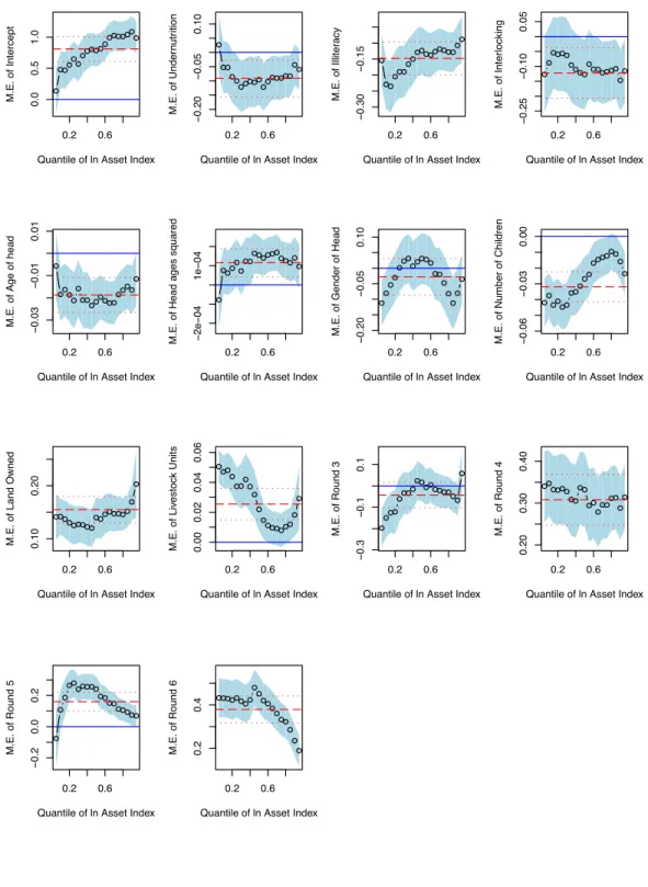
Figure 6: Quantile Regression:the Enset Area
0.2 0.6
0.0
0.5
1.0
Quantile of ln Asset Index
M.E. of Intercept ● ●●● ● ● ●●●●● ●●●●●● ● ● 0.2 0.6 − 0.20 − 0.05 0.10
Quantile of ln Asset Index
M.E. of Under n utr ition ● ●● ● ● ●●●● ● ●● ●●●●● ● ● 0.2 0.6 − 0.30 − 0.15
Quantile of ln Asset Index
M.E. of Illiter acy ● ●● ●●● ●● ●●●●●●●●●● ● 0.2 0.6 − 0.25 − 0.10 0.05
Quantile of ln Asset Index
M.E. of Inter locking ● ● ●●●● ● ●●●●●● ●●●● ● ● 0.2 0.6 − 0.03 − 0.01 0.01
Quantile of ln Asset Index
M.E. of Age of head
● ●●● ● ● ●● ●● ● ●●●● ●●● ● 0.2 0.6 − 2e − 04 1e − 04
Quantile of ln Asset Index
M.E. of Head ages squared
● ●●●●● ●●●●●●●●●●●● ● 0.2 0.6 − 0.20 − 0.05 0.10
Quantile of ln Asset Index
M.E. of Gender of Head
● ● ● ● ●●●●●●●● ●● ● ● ● ● ● 0.2 0.6 − 0.06 − 0.03 0.00
Quantile of ln Asset Index
M.E. of Number of Children
●●●●●● ●●● ●● ●●●● ●● ● ● 0.2 0.6 0.10 0.20
Quantile of ln Asset Index
M.E. of Land Owned
●●● ●●●●●●●● ●●●●●● ● ● 0.2 0.6 0.00 0.02 0.04 0.06
Quantile of ln Asset Index
M.E. of Liv estock Units ● ●● ● ●● ● ● ● ● ● ●●●●●● ● ● 0.2 0.6 − 0.3 − 0.1 0.1
Quantile of ln Asset Index
M.E. of Round 3 ● ●●● ●●● ● ●● ●●●●●● ●● ● 0.2 0.6 0.20 0.30 0.40
Quantile of ln Asset Index
M.E. of Round 4 ●● ●●●● ●● ●● ●● ●●● ●● ● ● 0.2 0.6 − 0.2 0.0 0.2
Quantile of ln Asset Index
M.E. of Round 5 ● ● ● ●●●●●●● ●● ●● ●●●●● 0.2 0.6 0.2 0.4
Quantile of ln Asset Index
M.E. of Round 6 ●●●●●●●● ● ● ●● ● ● ●● ● ● ●
most deprived region (the enset area) has evidence of interlocking poverty traps. Hence, we first focus on local levels. Figure 5 and Figure 6 represent distributions of marginal effects on the log
of structural income in the highlands region and the enset region, respectively.33 We find that
livestock units have a significantly positive and very heterogenous effects, while land owned has a significantly positive and relatively uniform effect over the whole range of the structural income distribution. The number of children within a household significantly worsens the household asset condition. Age of household heads has a negative and relatively unform effect. The effect of gender of the household head represents a different pattern between the highlands area and the enset area. The gender effect is negative and relatively uniform over the whole distribution in the highlands area, while the effect is significantly negative only in the lower percentile of the distribution in the enset area. The illiteracy trap has a significantly negative and very heterogeneous effect on the percentage change in the structural income in the enset area, but in the highlands area, it is insignificant for nearly all quantiles. An undernutrition trap has a relatively uniform effect on the structural income. Moreover, the impact of an undernutrition trap is marginally significant at 0.1 level over the whole range of the distribution in the highlands area; but it is significant in the enset area except at the highest and lowest percentiles of the income distribution.
In the highlands area, the interlocking poverty trap has an insignificant effect on log of asset index except among the lower percentiles of the distribution. Even though the differ-ences between the percentage change in the structural income of the trapped and that of the non-trapped households are significant in the lower percentiles of the income distribution, the differences between the absolute income levels of the trapped and those of the non-trapped
households are negligible.34 We conclude that an interlocking trap does not have significant
effects on the structural income of the households in the highlands area. In the enset area, however, an interlocking trap has heterogeneous effects on the percentage change in the struc-tural income over the income distribution. The percentage change in the income of the trapped households is not significantly different from that of the non-trapped households in the lower percentiles (i.e., below about 50th percentile), while the percentage change in the income of the trapped households is significantly less than that of the non-trapped households in the upper percentiles. This finding implies that there is household heterogeneity in the enset area in the
impact of interlocking poverty traps over the income distribution.35
We estimate the equation (4) again to compare the effects of each poverty trap indicator on household structural income at local levels with those in combined samples, treating all regions
as homogeneous. (See Figure A-8 in the Appendix to see the estimation results.36) We also
find heterogeneous effect of an illiteracy trap. It uniformly reduces about 15% of the structural
income for the poor.37
From the pseudo-fixed effect model and the quantile regressions, we have found that multi-dimensional, or interlocking poverty traps are likely to affect more severely households in the lower income distribution residing in the more deprived region. For additional evidence on the existence of multidimensional, and interlocking poverty traps, we revisited the estimation of the asset dynamics using nonparametric local linear regressions using ERHS round 1, 3, 4, 5,
and 6 data, which are used in Table 2.38 We estimate three asset dynamics according to trap
status: No-trap, single trap, and double trap.39
Table 2 gives a hint that there is complementarity of household resources in asset accu-mulation. Based on the findings in that table, we construct the following working hypothesis: First, if the dynamics of the single trapped group and the no-trapped group converge to the same equilibria, other resources in households work as substitutes for the trapped resource. Similarly, if the dynamics of the double trapped and the no-trapped groups converge to the same equilibrium, other resources in households work as substitutes for the trapped resource. However, if the dynamics of the non-trap group and single trap group converge to different equilibria; or if the dynamics of the non-trap group and double trap group converge to different equilibria; the significant difference of equilibria suggests that the lacked resources (trapped capacities or other assets) work with complementarity to hinder household asset accumulation. We hypothesize that this complementarity is more likely to appear in the most impoverished area. If the dynamics of the single or double trapped group converge to a very low equilibrium distinguished from the equilibrium of non-trapped group’s dynamics, we may conclude that multidimensional and interlocking traps exist since this complementarity involves the existence of interlocking traps.
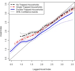
Figure 7 represents the asset dynamics of each trap status estimated with a local linear
par-Figure 7: Asset Dynamics across Trap Status: All Areas
ticularly around their own equilibria. The clearest difference is observed in the dynamics of the most-asset poor (with a lagged asset index of approximately 0 to 1.7). This difference implies that trap status tends to affect only the very asset-poor, which conforms with our interpreta-tion of Figure A-6, as well as Table 4. This finding may suggest that missing resources in a household asset growth function only determine the asset accumulation of the very poor.
Poverty could appear differently at local levels. As Table 2 suggests, the poor area has a much higher likelihood of complementarity of inputs in a household asset growth function. Hence, we investigate how trap status (or chronically lacking resources) hinders poor house-holds from asset accumulation. We do so by estimating nonparametric local linear regressions according to trap status (no, single, and double trap). Particularly, we focus on the enset and the highlands areas.
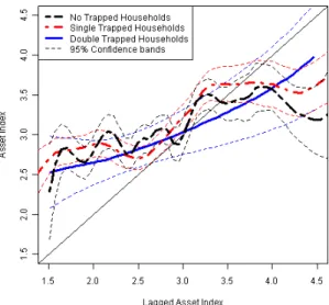
Figure 8 presents the asset dynamics across trap status in the enset area. We find that the dynamics of no-trapped household converge to the highest equilibrium, while the dynamics of
the double trapped households converge to the lowest equilibrium.41 Moreover, the dynamics
of single trapped households also converge to a significantly lower equilibrium than that of no-trapped households. However, we fail to observe these changes of dynamics depending on
trap status for the highlands region as seen in Figure 9.42 All dynamics in Figure 9 converge
Figure 8: Asset Dynamics across Trap Status in the Enset Area
Figure 9: Asset Dynamics across Trap Status in the Highlands Area
lack of one resource or even two resources, does not necessarily prevent households from asset accumulation since other surplus resources can make up for it in the long run. In the most impoverished area, however, the dynamics are clearly distinguished from each other. The interpretation in this case is that the lack of one resource makes the asset dynamics converge to the lower equilibrium. The households in the poorest area may have little surplus resources to make up for the missing resource. Lack of one resource in the end makes other resources unproductive so that the asset dynamics converges to a lower equilibrium than no-trapped households. This complementarity suggests the existence of multidimensional and interlocking poverty traps. Moreover, the stable equilibrium of the double trapped households is identified at about 1.3. The implied equilibrium is less than $1 per day, which may be readily interpreted
as an asset poverty trap.43
Therefore, we conclude that the interlocking effect of the traps is likely to appear in the most deprived area. We find that it is hard to distinguish the effect of each poverty trap on the dynamics of the non-poor area or the non-poor. This implies that the surplus resources that they have work as substitutes in the household asset growth function. From these results it may be inferred that the dynamics of the poor are not likely to converge with those of the non-poor in the long run when multidimensional and interlocking poverty traps exist. Hence, the hypothetical
explanation could be rejected that neither trap status determines the asset dynamics of rural Ethiopia. In addition, we may interpret the lowest stable equilibrium of the double trapped households as a form of multidimensional poverty trap. Since the multidimensional poverty traps affect the asset dynamics in the most deprived region, and hinder households from the accumulation of assets, we finally conclude that interlocking poverty traps do exist in the most impoverished region of Ethiopia.
7
Concluding Remarks
In this paper, we have considered the presence of multiple poverty dimensions. In addition to low-consumption (assets), we considered health traps as proxied by continued low BMI-for-age z scores, and education traps as proxied by continued illiteracy.
Estimating long term asset dynamics with the full sample, we fail to find evidence that the asset dynamics of the single trap households (i.e. either in an illiteracy or an undernutrition trap but not both), on average, differ from those of the non-trapped households. Considering differences at the regional level, however, we find evidence that the dynamic paths in the poorest region (enset growing area) represent different patterns depending on the trap status: First, the equilibrium is much lower than in two other regions; furthermore, the dynamics of the non-illiteracy group is located above that of illiteracy trap group.
However, the results from conditional mean regressions do not fully represent the behavior of the poor located in left tails of the structural income distribution. Considering long term differences across the structural income distribution, we adapt nonparametric quantile regres-sion. We first examine the full sample according to the trap status. The patterns of asset dynamics are significantly different according to the presence of an illiteracy trap only below the 40th percentiles of the income distribution. That is, the dynamics of the households in lower income fractiles (above the 50th percentile of the income distribution) converge to the same equilibrium regardless of illiteracy trap status, but the dynamics of the households in the lower income fractiles in an illiteracy trap converge to a lower equilibrium than households in similarly low parts of the income distribution not having an illiteracy trap.
level. We further examined the possibility that there are interlocking traps, in the sense that low levels of health and education have a negative interaction effect on assets. We find this effect in the most deprived region: both illiteracy and undernutrition trapped households have significantly less assets than the counterparts; and there is a statistically significant negative interaction effect of illiteracy and undernutrition on assets. In highlands area, only the under-nutrition trap status variable has a marginally significant negative effect on assets, but there is no significant interaction effect. In the hoe area, we also fail to find evidence of a significant negative interaction effect.
Considering short term differences across the structural income distribution at the regional level, results from quantile regressions show that the significance of each trap differs across regions over the income distribution. In particular, in the highlands (the region with the best technology and resources) an illiteracy trap has no significant impact on asset change across the asset distribution. However, in the enset (most deprived) region, an illiteracy trap has a significantly negative effect on asset change, and the effects are very heterogeneous over the asset distribution. These results are suggestive that policy and programs should be attuned to whether the poor are trapped and in what ways.
In section 2, we argue that health and education, for example, to a degree might act as substitutes for each other in allowing the accumulation of assets, but when both are lacking this may prevent accumulation since the very poor have only very small amount of other assets that might otherwise work as substitutes for the lacking resources. That is, with high deprivations, all resources turn out to be complementary inputs for asset production. The existence of this complementarity is itself further evidence of interlocking poverty traps.
Therefore, we re-examined the long term asset dynamics, to further investigate the presence of interlocking poverty traps at the regional level. We find that asset dynamics in the most deprived region is distinguished from those of other areas: the estimated dynamics in the most impoverished area are separated out according to the trap status (no, single, and double trap), while all the asset dynamics estimated in other areas converge to statistically the same equilibrium. Only in the enset area are the dynamics of no-trapped, single-trapped, and double trapped households all statistically different: the equilibrium of the double trapped group is statistically below that of the single-trapped groups, which in turn are below the equilibrium of
the non-trapped group. This finding supports that household inputs turn out to be complements in the most impoverished area, when a set of household resources is lacking. Therefore, the most impoverished area has the highest likelihood that the multidimensional, and interlocking poverty traps are found.