Utility based Data Mining for Time Series Analysis -
Cost-sensitive Learning for Neural Network Predictors
Sven F. Crone
Lancaster UniversityDepartment of Management Science Lancaster, LA1 4YX, UK
+44 1524 592991
[email protected]
Stefan Lessmann
University of Hamburg Institute of Information Systems VMP 5, 20146 Hamburg, Germany+49 40 42838-5500
[email protected]
Robert Stahlbock
University of Hamburg Institute of Information Systems VMP 5, 20146 Hamburg, Germany+49 40 42838-3063
[email protected]
ABSTRACT
In corporate data mining applications, cost-sensitive learning is firmly established for predictive classification algorithms. Conversely, data mining methods for regression and time series analysis generally disregard economic utility and apply simple accuracy measures. Methods from statistics and computational intelligence alike minimise a symmetric statistical error, such as the sum of squared errors, to model ordinary least squares predictors. However, applications in business elucidate that real forecasting problems contain non-symmetric errors. The costs arising from over- versus underprediction are dissimilar for errors of identical magnitude, requiring an ex-post correction of the prediction to derive valid decisions. To reflect this, an asymmetric cost function is developed and employed as the objective function for neural network training, deriving superior forecasts and a cost efficient decision. Experimental results for a business scenario of inventory-levels are computed using a multilayer perceptron trained with different objective functions, evaluating the performance in competition to statistical forecasting methods.
Categories and Subject Descriptors
H.2.8 [Database Management]: Applications – Data Mining
General Terms
Algorithms, Management, Economics
Keywords
Data Mining, cost-sensitive learning, asymmetric costs, neural networks, time series analysis
1.
INTRODUCTION
Profit and costs drive the utility of every corporate decision. As corporate decision making, from strategic to operational planning, is based upon future realisations of the decision parameters, e.g. telecommunications demand [1] or the likelihood of responders
reacting to a mailing campaign [2], predictions or forecasts are a prerequisite for all managerial decisions. The quality of a forecast must be evaluated considering its ability to enhance the quality of the resulting decision. In management decisions, the utility arising to the decision maker from decisions based upon sub-optimal forecasts is measured in profit and costs. As a consequence, costs need to be incorporated to guide the predictions and ultimately derive valid corporate decisions.
In predictive data mining, the relevance of incorporating the costs resulting from a decision is reflected in approaches of cost-sensitive learning [3]. For classification, the costs for accurately predicting class membership of instances are proportional to the amount of accurately predicted instances. In addition, the costs associated with true versus false prediction of positives and negatives are often asymmetric [4] and are routinely used to guide the parameterisation and selection process of a wide range of classifiers, e.g. MetaCost [5] or cost sensitive boosting [6]. Consequently, robust evaluation techniques like the ROC convex hull method [7, 8] or the area under the ROC curve [9] have been proposed to enable classifier assessment in accordance with managerial objectives.
Similarly, for the predictive data mining problems of regression and time series analysis [10, 11] the costs arising from invalid point prediction of the true realisation increase with the magnitude of the error. In addition, the costs of the decisions derived from positive versus negative errors, or underprediction versus overprediction, are also often asymmetric. For example, in inventory management of retail outlets, keeping units of consumer goods in stock or on shelf in order to satisfy customer demand the effect of overstocking a product may induce increased stock holding costs for a single period versus the costs of understocking leading to lost sales revenue and dissatisfied customers. In both cases, the final evaluation of a forecast must be measured by the monetary costs arising from setting suboptimal decisions based on imprecise predictions of future demand [12], for asset transactions or inventory levels alike. Consequently, they depend on the given decision environment and a chosen behavioural strategy resulting from the decisions. These costs arising from over- and underprediction are typically not quadratic in form and frequently non-symmetric [13]. In addition, it is the asymmetry of costs that determines corporate policy, e.g. setting a target of satisfying 95% of demand.
However, for regression problems these asymmetries are largely neglected. Particularly in the field of data driven time series
© ACM, 2005. This is the author’s version of the work. It is posted here by permission of ACM for your personal use. Not for redistribution. The definitive version was published in
UBDM ’05, August 21, 2005, Chicago, Illinois, USA. Copyright 2005 ACM 1-59593-208-9/05/0008 …$5.00. http://doi.acm.org/10.1145/
analysis and prediction, predictors of continuous scale are routinely evaluated using accuracy based evaluations through statistical error measures, such as the mean squared error or absolute error, eluding the reality of asymmetric costs of over- and underprediction. While this may seem unsurprising in the domain of econometric modelling of conventional statistical methods such as regression, autoregressive methods and exponential smoothing, these practices also persist in the domain of novel methods from computational intelligence, permitting minimisation of arbitrary objective or error functions through adaptive learning algorithms. Artificial neural networks (NN) have found increasing consideration in forecasting theory, leading to successful applications in time series and explanatory sales forecasting [14, 15]. Based upon modest research in non-quadratic error functions in NN theory [15, 16] and asymmetric costs in prediction theory [13, 17-19], a set of asymmetric cost functions was recently proposed as objective functions for neural network training [20]. In this paper, we analyse the efficiency of a linear asymmetric cost function in inventory management decisions, training a multilayer perceptron to find a cost efficient stock-level for a set of seasonal time series directly from the data. As a consequence, the NN is trained directly using the ideas developed in utility based or cost-sensitive learning within the data mining domain.
Following a brief introduction to neural network prediction in inventory management, Section 3 assesses statistical error measures and asymmetric cost functions for neural network training. Section 4 gives an experimental evaluation of neural networks trained with asymmetric cost functions, outperforming expert software-systems for time series prediction. Conclusions are given in Section 5.
2.
NEURAL NETWORK PREDICTIONS
FOR INVENTORY DECISIONS
2.1
Forecasting for inventory management
In inventory management, forecasts of future demands are generated to select an efficient inventory level, balancing inventory holding costs for excessive stocks with costs of lost sales-revenue through insufficient stock [21, 22]. Although the amount of costs will generally increase with the numerical magnitude of the forecast errors, the costs arising from over- and underprediction are frequently neither symmetric nor quadratic [12, 19].
A service-level is routinely determined from strategic objectives or according to the actual costs arising from the decision, e.g. aiming to fulfil 98.5% of customer demand to balance this trade-off. Assuming Gaussian distribution, setting the inventory level to the optimum predictor will only fulfil 50% of all customer demand. Therefore, safety-stocks are calculated to reach the service level, using assumptions of the conditional distribution of the ex post forecast errors of the method applied [22].
For the decision of an inventory level for a single product in a single period of time the classic “newsboy”-problem is applicable. The decision rule for a service level resulting from a given cost of underprediction cu and overprediction co reads
( )
o u u y c c c Q p + = < * , (1)giving the value for a lookup of k in the probability table of the valid distribution, with
p
( )
denoting the probability of sales ybeing lower than an optimal inventory quantity Q* held in each period. The final stock-level s is calculated using the forecast
ˆ
t hy
+ of the sales volume y and adding a safety stock (SS) of kstandard deviations of the forecast errors [22]:
e h
t
k
y
s
=
ˆ
++
δ
. (2)Consequently, the precision of the forecasts directly determines the safety stocks kept, the inventory level and the inventory holding costs. Hence, forecasting methods with superior accuracy such as NN may significantly reduce inventory holding costs [22].
2.2
Neural networks for time series analysis
Forecasting time series with non-recurrent NNs is generally based on modelling the network in analogy to a non-linear autoregressive AR(p) model [23]. At a point in time t, a one-step ahead forecast yˆt+1 is computed using n observations
1
1, ,
, t− t−n+
t y y
y from n preceding points in time t, 1, t-2, …, t-n+1, with n denoting the number of input units of the NN. This models a time series prediction of the form
(
1 1)
1
,
,...,
ˆ
t+=
f
y
ty
t−y
t−n+y
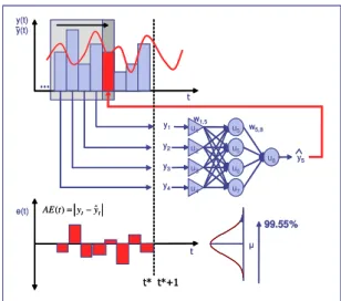
. (3)The architecture of a feed-forward multilayer perceptron (MLP) of arbitrary topology together with the resulting residuals of invalid forecasts denoted as the absolute error (AE) is displayed in Fig. 1.
y(t) y(t) u5 u5 u6 u1 u2 u3 u4 u7 u8 w5,8 y5 y1 y2 y3 y4 w1,5 t t y y t AE()= −ˆ e(t) 99.55% y(t) y(t) u5 u5 u6 u1 u2 u3 u4 u7 u8 w5,8 y5 y1 y2 y3 y4 w1,5 t t y y t AE()= −ˆ e(t) 99.55%
Figure 1. Neural network application to time series forecasting in inventory management, applying a MLP with 4 input units
for observations in t, t-1, t-2, t-3, 4 hidden nodes and 1 output node for time period t+1.
The task of the MLP is to model the underlying generator of the data during training, so that a valid forecast is made when the trained network is subsequently presented with a new value for the input vector [16]. Therefore the objective function used for NN training determines the resulting system behaviour and performance [15].
The objective functions routinely employed in neural network training differ from the objective function of the underlying
inventory management decision in slope, scale and ratio of asymmetry. Following, alternate objective functions are discussed to incorporate the original objective structure in NN training.
3.
OBJECTIVE FUNCTIONS FOR
COST-SENSITIVE REGRESSION LEARNING
Supervised online-training of a MLP is the task of adjusting the weights of the links wij between units i,j and adjusting their
thresholds to minimise the error
δ
j between the actual and adesired system behaviour [24]. Gradient descent algorithms traditionally minimise the modified sum of squared errors (SSE)
as the objective function, ever since the popular description of the back-propagation algorithm by Rumelhart, Hinton and Williams [25].
The SSE, as all statistical error measures, produces a value of 0 for an optimal forecast and is symmetric about et=0, implying
symmetric costs of errors in predicting future demand for inventory levels. The consistent use of the modified SSE in time series forecasting with NN is motivated primarily by analytical simplicity [15] and the similarity to statistical regression problems, modelling the conditional distribution of the output variables [24]. As neural network theory and applications consistently focus on the symmetric SSE-function for training, therewith modelling least squares predictors as well, the forecasts also need to be adjusted using safety stocks to attain a desired service-level.
Following, we propose an asymmetric cost function (ACF), modelling the objective function of the costs arising in the original decision problem instead of least squares predictors. These costs are often not only quadratic, but also non-symmetric in form. The objective function in NN training, determining the size of the error in the output-layer, may thus be interpreted as the actual costs arising from an overprediction or an underprediction of the current pattern p, comprising all input and output information for the MLP, in training.
Recently, we introduced a linear ACF to NN training [20], originally developed by Granger for statistical forecasts in inventory management problems [19]. The LINLIN cost function
(LLC) is linear to the left and right of 0. The parameters a and b
give the slopes of the branches for each cost function and measure the costs of error for each stock keeping unit (SKU) difference between the forecast yˆt+h and the actual value yt+h. The
parameter co corresponds to an overprediction and the resulting
stock-keeping costs, while cu relates to the costs of lost
sales-revenue for each underpredicted SKU. The LLC yields:
ˆ for ˆ ˆ ˆ ( , ) 0 for ˆ for ˆ o t h t h t h t h t h t h t h t h u t h t h t h t h c y y y y LLC y y y y c y y y y + + + + + + + + + + + + − < = = − > . (4)
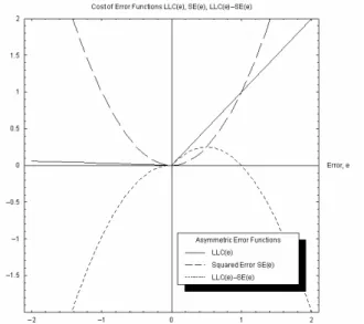
The shape of one asymmetric LLC, as a valid linear approximation of a real cost function in our corresponding inventory management problem, is displayed in Fig. 2.
Figure 2. Empirical Asymmetric Cost Function showing cost arising for over- and under-prediction, using co=£0.01 and
cu=£1.00 in comparison to the SE.
For
c
u≠
c
o these cost functions are non-symmetric about 0 and are hence called asymmetric cost functions. The degree of asymmetry is given by the ratio of co to cu[17]. For co = cu =1 theLLC equals the statistical absolute error measure AE. The linear form of the ACF represents constant marginal costs arising from the business decision. Our model therefore coincides with the analysis of business decisions based on linear marginal costs and profits.
Yang, Chan and King introduce a classification-scheme for objective functions, introducing dynamic non-symmetric margins for support vector regression [17]. Applied to objective functions in NN training it allows a classification of all symmetric statistical error functions and asymmetric cost functions previously developed. Linear, non-linear and mixed ACFs have been specified in literature [13, 17-19] while variable or dynamic objective functions to account for varying or heteroscedastic training objectives have not yet been developed for NN-training, as shown in Table 1.
Table 1. Objective functions for neural network training Symmetry of objective function Variability
Symmetric Non-symmetric
Fixed statistical error functions SE, AE, ACE. asymmetric cost functions LINLIN etc.
Variable - -
Asymmetric transformations of the error function alter the error surface significantly, resulting in changes of slope and creating different local and global minima. Therefore, using gradient descent algorithms, different solutions are found minimising cost functions instead of symmetric error functions, finding a cost minimum prediction for the inventory management problem. These asymmetric cost functions may be applied in NN training using a simple generalisation of the error-term of the back-propagation rule and its derivatives, amending only the error calculation for the weight adaptation in the output layer [20], but
applying alternative training methods or global search methods to allow network training [15]. For the following simulation experiments, we developed a simulator allowing minimisation of arbitrary, non-differentiable objective functions through the use of gradient decent and code controlling for non-defined derivatives.
4.
SIMULATION EXPERIMENT OF
COST-SENSITIVE TIME SERIES ANALYSIS
4.1
Experimental time series data
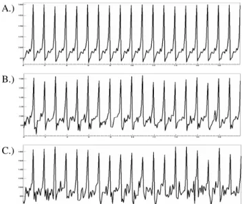
Following, we conduct an experiment to evaluate the ability of a MLP to evolve a set of weights minimising an LLC asymmetric cost function for a seasonal time series. We analyse a set of benchmark time series for seasonal time series prediction recently published in a study by Zhang and Qi [26]. In order to exemplify the potential impact of asymmetric cost functions in an empirical setting while controlling for problems of model misspecification and selection, we limit our analysis to the three artificial time series, closely resembling the seasonality and length of real department store sales [26]. The simulated series were created using a multiplicative seasonal model without trend
100
t t t
y = SI +E , (5)
with SIt the seasonal index for each month, Et the additive error
term following a normal distribution
N
( )
0,
µ
and t denoting the time index. The seasonal indices to calculate each observation are{
.75;.80;.82;.90;.94;.92;.91;.99;.95;1.02;1.20;1.80}
t
SI = . (6)
To estimate the effect of different noise levels on the forecasting accuracy the authors apply three levels of error variance
σ
2=
{
1;25;100
}
to construct three time series A, Band C. A total of 1200 points is generated for each time series of a particular noise level. In order to control for external influences we sourced the original time series from the authors, to realign the properties of the random noise with the original series. A part of the time series is presented in Figure 3.
A.)
B.)
C.)
Figure 3. Part of three artificial time series A, B and C.
An analysis of the autocorrelations (AC) and partial autocorrelations (PAC) reveals the purely seasonal pattern of the time series. An analysis of the noise reveals the structure documented by Zhang and Qi and no significant AC or PAC.
Figure 4. Autocorrelation function and partial autocorrelation function of the seasonal SIt without added noise.
The autocorrelation function (ACF) of the undifferenced series of the seasonal factors without noise reveals a seasonal pattern with significant spikes at lagged 12 months apart with decaying magnitude, indicating a seasonal autoregressive process an the absence of a moving average process. As expected, first seasonal differencing D=1 eliminates all AC and PAC across all lags. Similarly, for all three noisy time series first seasonal differencing eliminates all significant ACs and PACs at all lags.
4.2
Objective functions
To exemplify the effect of different objective functions on NN predictions, we compare three objective functions. Firstly, we train a set of NN using a squared error (SE) objective function, NNSE, modelling least squares predictors to find the mean of the
distribution, implying equal costs cu=co=1 and 50% service level.
Secondly, we train a set NNLLC-1 using an asymmetric cost
function to reflect the estimation of a cost efficient inventory level. In order to specify the underlying costs arising from the decision process we specify a particular cost trade-off reflecting an empirical cost relationships in fast moving consumer goods retailing, also reflecting the original motivation of the artificial time series from the retail domain. A retail outlet needs to allocate products to customer demand for each period. Overprediction of consumer demand leads to unsold items and inventory holding costs co for another period while underprediction results in costs
cu through lost sales-revenue per product, assuming cu>co and
disregarding fixed costs of the decision. As a consequence, we construct a newsboy decision problem, reflecting the single period inventory model without backordering, as outlined under section 2.1. We create an linear asymmetric cost function LLC-1 of (co=$0.1; cu=$1.00), implyinghigh costs of running out of stock
respectively. The asymmetric cost relationship relates to a 90% service level, by
( )
* 1.00 -1: 0.90 1.00 0.10 u y u o c LLC p Q c c < = + = + = . (7)In addition, we train a third set of NNLLC-2 using an objective
function LLC-2 of (co=$1.00; cu=$0.10) implyinghigh costs of
overstocking as the reverse quantile of LLC-1, as in
( )
* 0.10 -2 : 0.10 0.10 1.00 u y u o c LLC p Q c c < = + = + = . (8)While a 10% service level seems implausible from a corporate policy perspective, it may serve to evaluate the NN ability to estimate arbitrary quantiles on both sides of distribution.
4.3
Design of the forecasting methods
Each of the three time series of n=1200 observations is split into three disjoint datasets for NN training, validation and testing, using the last 300 observations for out-of-sample evaluation in the test dataset, 300 observations for early stopping and selection of the best NN model in the validation dataset and the rest of the 600 observations for parameterisation in the training dataset. This results in 588, 300 and 300 predictable patterns in each set. Considering the limited length of the time series for training and testing, only an approximation and no exact estimation of the quantile and service level minimizing the costs appears feasible. All data was scaled from a range of 0 to 210 into the interval [-1;1] applying a headroom of 20% to avoid saturation effect of the nonlinear activation functions. It should also be noted, that the ability of NN to forecast seasonal and trended time series patterns has recently been questioned [26], leading to recommendations to deseasonalise and detrend time series prior to training the networks. With regard to our own research findings we refrain from preprocessing the time series this way, and train the NN on the original, seasonal auto regressive patterns.
To determine an efficient and parsimonious network architecture while limiting experimental complexity, we pre-evaluated a set of input vectors applying different lag structures from {t-1,…t-36}, a number of {0…20} nodes in a single hidden layer with different sigmoid activation functions {tanh; logistic} and different output functions in the output layer {tanh; logistic; identity} simultaneously. We evaluated 594 network topologies on 10 initialisations each with randomised starting weights to account local minima. The results were analysed conducting a multifactorial analysis of variance (ANOVA) with equal cell sizes to identify significant suboptimal topologies. While topologies with 0 or 1 hidden nodes showed reduced accuracy, no significant differences between topologies with hidden nodes n>2 could be identified using a multiple comparison test of homogeneous subgroups of estimated marginal means. The impact of activation functions showed a negative effect of the sigmiod function in the output layer and a negative interaction effect between tanh and non-tanh functions in the output layer. It found no significant difference in performance between tanh in both hidden and output layer and sigmoid in hidden and identify in the output layer. As a consequence, we selected the most parsimonious topology with the lowest MSE and variance on the validation dataset for further experimentation. We chose a fully connected MLP without
shortcut connections, applying a topology of 12 input nodes for the time lags t-1,…,t-12 to exploit all feasible yearly time-lags of a monthly series, 2 hidden nodes and 1 output node. Additionally, one bias unit models the thresholds for all units in the hidden and output layer. All units in the hidden layer use a summation as an input-function, the logistic function as a semilinear activation function and the identity function as an output function. The unit in the output layer uses a nonlinear, unbounded identity function. Three sets of networks NNSE, NNLLC-1 and NNLLC-2 were trained
using different objective functions. Each MLP was initialised and trained for twenty times to account for [-0.6;0.6] randomised starting weights. We applied a standard backpropagation algorithm, using an initial learning rate of =0.5 decreased by a cooling factor of .99 after every epoch, and a momentum term of
ϕ=.4. Training consisted of a maximum of 1000 epochs with a validation after every epoch, applying early stopping if a composite of 50% training and 50% validation error did not decrease by 0.01% for 10 epochs. After training a total of 189 NN across 3 time series and for 3 objective functions, the results for the best network within each subgroup, chosen on its objective function performance on the validation set, was computed for all three data subsets. Consequently, NNSE was selected on lowest
mean squared error (MSE) on the validation set, NNLLC-1 on
lowest mean LLC1 and NNLLC2 on lowest mean LLC2 on the
validation set respectively. Only the test dataset is used to measure generalisation, applying a simple hold out method for out-of-sample evaluation or generalisation.
To compare the performance on achieving a 90% service level, we need to extend the NNSE predictions through the calculation of
safety stocks. We generate business forecasts based upon ordinary least-squares predictors of the best NNSE and conventional
statistical methods and calculate additional safety stocks necessary to achieve the desired service level using the standard formulas. As statistical benchmarks, the Naïve1 method using last periods sales as a forecast,
y
ˆ
t+1=
y
t, exponential smoothing and ARIMA were computed. The statistical predictions were computed using the benchmark software system Forecast Pro, which selects and parameterises appropriate models of exponential smoothing or ARIMA intervention models based upon statistical testing and expert knowledge based on the properties of each time series [27]. For the predictions by NNSE and the Naïve method the finalinventory level was calculated as in ForecastPro, using
ˆt h 2.33 e
s y= + +
σ
, (9)for an ex-post correction of the ordinary least squares predictor by adding k=2.33 standard deviations σ to derive a cost efficient service level of 90.0% for the given inventory problem, assuming Gaussian distribution and homoscedastiticity of the residuals, as confirmed by Kolmogorov-Smirnov tests.
In contrast, the asymmetric cost predictor NNLLC-1 was trained to
predict the cost efficient inventory level, equal to a 90% service level, for each month directly from the training process. Following the experiments we assess the ex-post performance of the competing approaches in the following section.
All neural network experiments were computed using the NN software simulator “Intelligent Forecaster”, developed within our research group to compute and compare multiple NN time series experiments on arbitrary objective functions. Average runtime for
training a NN, creating predictions and saving results was 2.75 seconds on a Pentium IV 3.8 GHz, 4GB RAM, 1TB disk drive.
4.4
Experimental impact of cost functions
First, we evaluate the ability of a NN to estimate a predetermined service level from the cost relationship of over- versus underprediction. Consequently, we compare the forecasts and resulting service levels of the three sets of NNs to evaluate their ability to adhere to different objectives during the training process across the three time series.
Table 2 displays the results using mean error measures computed on each dataset to allow comparison between datasets of varying length. The results are given in the form (training set / validation set / test set) to allow interpretation. The descriptive performance measure of the alpha-service-level gives the amount of suppressed sales occurrences per dataset. All methods are evaluated ex-post on their performance by mean SE(MSE) and the ex post mean
LINLIN costs (MLLC) for each objective function MLLC-1 and
MLLC-2 respectively. In addition, the NN predictions on the test set for out-of-sample evaluation are presented in figures. The results reflect the impact of different objective functions SE, LLC-1 and LLC-2. Each set of NN shows lower mean errors or costs across all time series A, B, and C for its individual training objectives. E.g. NNSE shows significantly lower MSE then
NNLLC-1 and NNLLC-2. Vice versa, NNLLC-1 shows robust
minimisation of MLLC-1 in- and out-of-sample as opposed to both other sets of trained networks. These results are confirmed in a multifactorial ANOVA, revealing two homogeneous subsets of the method trained on minimising the particular error measure versus the two other methods. An analysis of the service levels further reveals, that each method approximates the target service level of 50%, 90% and 10% within and out-of-sample robustly and accurately, considering the achievable degree of accuracy determined through the length of the time series. We may therefore conclude, that NN allow minimisation of arbitrary objective functions to estimate different service levels.
Various additional results may be drawn from the experiment. As expected, the best selected NNSE trained on the standard SE
approximates the seasonal time series pattern and generates valid and reliable t+1 predictions on validation and test dataset across all three time series, as visible in the results of Table 2 and the part of the test set predictions given in Figure 5. With regard to the decreasing signal to noise ratio the predictions show increasing deviations from the actual data from time series A to B and C, as must be expected.
Figure 5. Predictions of a NNSE trained on minimising the symmetric SE to forecast monthly retail sales across three time series A, B and C from above. The graph shows the time series of retail demand in blue versus the NN forecast in red on the
test dataset.
Nevertheless, the artificial data pattern underlying the generated time series is robustly extracted by NNSE regardless of the
increasing noise level, demonstrating only limited overfitting through the training process. In cost and inventory terms, the NN are trained on equal costs of over- versus underprediction in order to estimate a 50% service level relating to the ordinary mean predictor, as shown in Figure 5. As a consequence, we are unable to confirm recent findings in the forecasting and management science domain, that NN are incapable of predicting seasonal time series patterns without prior deseasonalisation.
The level of predictions given by the NNs trained on minimizing the asymmetric cost function LLC-1 presented in Figure 6 differs significantly from the predictions by the NNSE. Analysing the
behaviour of the forecast based upon the asymmetry of the costs function, the neural network NNLLC-1 raises its predictions in
comparison to the NNSE trained on squared errors to achieve a
cost efficient forecast of the optimum inventory level. Predictions on the test set are displayed in Figure 6, with identical patterns on the training and validation set omitted due to the length of the time series and space restrictions.
Table 2. Results on Forecasting Methods and NNs trained on linear Asymmetric Costs and Squared Error Measures
Error Measures Service Level
Objective
Function Series NN no. Time MSE(e) MLLC-1 (e) MLLC-2 (e) alpha
NNSE A (#30) 1.35 1.45 1.23 .47 .51 .43 .55 .55 .54 50.9% 49.0% 54.0% B (#96) 26.63 28.00 30.17 2.26 2.14 2.56 2.27 2.44 2.26 49.7% 50.0% 47.0% C (#147) 104.77 88.08 100.35 4.78 4.36 4.27 4.15 3.86 4.32 49.3% 49.7% 54.7% NNLLC-1 A (#53) 4.50 4.77 4.14 1.79 1.79 1.67 0.23 0.26 0.21 90.3% 87.3% 93.0% B (#98) 78.44 75.90 83.50 7.11 6.96 7.44 0.99 1.04 1.05 92.5% 91.7% 90.0% C (#158) 246.85 221.95 219.87 12.28 11.89 11.46 1.82 1.77 1.69 90.5% 91.7% 90.7% NNLLC-2 A (#1) 4.23 4.28 4.20 .22 .23 .21 1.68 1.66 1.72 7.3% 9.7% 6.7% B (#109) 81.93 84.16 76.71 .93 1.00 .96 7.25 7.50 6.90 7.7% 10.7% 6.3% C (#163) 267.46 251.13 279.30 1.84 1.69 2.00 13.14 12.99 13.73 9.4% 10.7% 13.7%
Figure 6. NNLLC-1 predictions on a part of the test dataset across time series A, B and C from top to bottom, aiming to minimise inventory costs through an service level of 90%. The upper red line denotes the forecasts, the lower blue the actuals.
The network accounts for higher costs of underpredicition versus overprediction through increased predictions, therefore avoiding costly stock-outs. The predictions estimate a cost minimal point depending on the varying distributions of the error residuals, as visible in level of predictions increasing with the size of the error distribution from time series A to C. This is also evident in the lack of stock-outs represented by the increased service-level of 93.0%, 90.0% and 90.7% on time series A, B and C.
To evaluate the validity and reliability of the NN training, we estimate an inverse ACF of the given problem domain, estimating the 10% quantile. As shown in Figure 7, the NN alters its estimation on asymmetric costs by lowering its predictions to robustly achieve a 10% service level across all three time series.
Figure 7. NNLLC-2 predictions on a part of the test dataset across time series A, B and C, aiming at a service level of 10%. The lower red line denotes the forecasts, the upper the actuals.
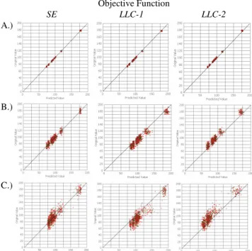
Consequently, a neural network may be trained to not only predict the expected mean of a time series but instead produces a biased optimum predictor, as intended by Grangers original work through ex post correction of the original predictor [19]. This may be interpreted as finding a valid approximation for a point on the conditional distribution of the optimal predictor depending on the standard-deviation, or quantile autoregression. Within an inventory management problem, the network finds a cost efficient inventory level without the separate calculation of safety stocks directly from the cost relationship. This reduces the complexity of the overall management process of stock control, successfully calculating a cost efficient inventory level directly through a forecasting method using only a cost function and the data. The results of the adjusted in relation to the increasing noise levels become visible in a PQ-scatterplott in Figure 8.
Objective Function SE LLC-1 LLC-2 A.) B.) C.)
Figure 8. PQ-scatter plots of actual values versus predicted values for three time series A, B and C and objective functions
indicating accuracy and lack of biases in predictions
A set of insignificant Kolmogorov-Smirnov tests confirms the normality of the residuals for all predictions, with the residuals of the NNSE being centred around zero while the residuals of
NNLLC-1 and NNLLC-2 are centred around the relevant quantile. As
a consequence we may use the standard formula to estimate the 90% quantile or service level to compare the methods performance on the estimated inventory levels in the next section.
4.5
Experimental accuracy of inventory levels
After determining the general ability of NN to predict a cost efficient inventory level for the newsboy problem directly through training with an asymmetric cost function, we seek to evaluate their accuracy in comparison to a conventional ex-post correction of the mean estimator of a statistical forecasting method.
We utilise the predictions of the NNSE for time series A, B and C
and add a safety stock of k=2.33 standard deviations to the individual prediction, in accordance with the Gaussian noise and
homoscedasticity of the residuals as confirmed by nonparameric testing. In addition, we use ForecastPro to generate statistical forecasts for each time series, selecting three different seasonal ARIMA (p,d,q)(P,D,Q) models all with log transform as optimum methods. For time series A, ForecastPro selects an ARIMA(2,0,2)*(0,1,1), for time series B an ARIMA(1,0,0)*(0,1,1) and an ARIMA(0,0,3)*(0,1,1) with log transform for time series C. In addition, the software uses an internal expert procedures for residual analysis and safety stock calculation to achieve a 90.0% service level based upon its forecasts and the adequate distribution of the residuals directly. We compute ex post accuracy on the business objective, using the actual costs occurring form each unit out-of-stock and each item left overstocked for each period t in the dataset, approximated by LLC-1. The ex-post costs arising from over- and underprediction alike represent the true variable decision costs and therefore a valid business objective in operational inventory management. In addition, we compute the number of stock-out and overstock occurrences to evaluate the frequency in which suboptimal decisions were made regardless of the magnitude of the errors. The results are provided in Table 3 with parts of the time series and calculated inventory levels provided in separate figures. Unsurprisingly, all methods outperform the benchmark naïve method, showing significantly better results through robust identification and extrapolation of the seasonal time series pattern in forecast and inventory levels.
The best NNLLC-1 trained with the asymmetric LINLIN cost
function LLC-1 gives an overall superior forecast regarding the business objective of minimising costs, achieving the lowest mean costs in-sample on training and validation data as well as out-of-sample on the test-data and across all three time series A, B and C. For the noisy time series C, it exceeds all inventory methods, and clearly outperforms forecasts of NN trained with the SE
criteria and added safety stocks, as presented in Figure 9. An analysis of the marginal means reveals two homogeneous subsets of costs. While the differences between NNLLC-1 and all other
methods prove statistically significant, no significant differences could be confirmed between NNSE forecasts and ARIMA forecasts
using the conventional calculation of safety stock.
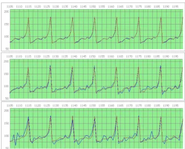
40 60 80 100 120 140 160 180 200 11 05 11 15 11 25 11 35 11 45 11 55 11 65 11 75 11 85 11 95 Actual NN + Safety Stock NN LLC-1
Figure 9. Comparison of predictions by NNSE plus 2.33 standard deviations of safety stock ( ) versus direct inventory
calculation by NNLLC-1 (∆∆∆∆) on time series C.
In addition, NNLLC-1 outperforms the best automatically selected
and parameterised ARIMA model and safety stocks selected by the software expert system, as displayed in Figure 10. Considering the inferior quality of the predictions provided by the Naïve method, its benchmarks may be excluded from further analysis.
35 85 135 185 235 11 05 11 15 11 25 11 35 11 45 11 55 11 65 11 75 11 85 11 95 Actual NN LLC-1 Naive Forecast Pro
Figure 10. Comparison of inventory levels from the Naïve method (€€€€) and ForecastPro (ΟΟΟΟ) plus 2.33 standard deviations
of safety stock ( ) versus NNLLC-1 (∆∆∆∆). on time series C.
Table 3. Results on Forecasting Methods and NNs trained on linear Asymmetric Costs and Squared Error Measures
Cost Error Measures Descriptive Error Measures of Inventory Holding
Sum of LLC-1(e,) with co=0.1; cu=1 No. of overstocked occurrences No. of out-of-stock occurrences
Time
Series Forecasting Method Training Validation Test Training Validation Test Training Validation Test
A NNLLC-1 inventory 129.95 68.61 64.49 531 262 279 57 38 21 NNSE + safety stock 163.74 82.80 85.05 586 289 289 2 2 2 ForecastPro 137.71 69.14 71.70 580 296 295 8 4 5 Naïve Method 4870.74 2495.11 2485.25 588 300 300 0 0 0 B NNLLC-1 inventory 558.57 299.74 291.20 544 275 270 44 55 30 NNSE + safety stock 725.51 379.59 364.92 587 297 298 1 3 2 ForecastPro 694.82 358.67 341.35 582 296 299 6 4 1 Naïve Method 5014.08 2557.91 2558.13 588 300 300 0 0 0 C NNLLC-1 inventory 1099.74 491.78 592.35 532 275 272 56 25 28 NNSE + safety stock 1361.14 689.33 734.17 580 297 294 8 3 6 ForecastPro 1257.56 655.08 684.18 578 298 294 10 2 6 Naïve Method 5171.19 2636.68 2642.80 587 300 298 1 0 2
40 60 80 100 120 140 160 180 200 11 05 11 15 11 25 11 35 11 45 11 55 11 65 11 75 11 85 11 95 Actual NN + Safety Stock NN LLC-1 Forecast Pro
Figure 11. Comparison of predictions by NNSE ( ) and a ForecastPro ARIMA model (ΟΟΟΟ) plus 2.33 standard deviations
of safety stock ( ) versus NNLLC-1 (∆∆∆∆) on time series B.
While these results prove consistent across all time series, the differences in prediction for time series B become smaller due to the reduced noise levels and prove insignificant in testing, also apparent in Figure 11 for time series B. For time series C of the lowest noise level, the differences in accuracy between the competing methods prove statistical non-significant. Nevertheless,
NNLLC-1 demonstrates a competitive performance in comparison
to established forecasting and inventory methods.
40 60 80 100 120 140 160 180 200 11 05 11 15 11 25 11 35 11 45 11 55 11 65 11 75 11 85 11 95 Actual NN + Safety Stock NN LLC-1 Forecast Pro
Figure 12. Comparison of predictions by NNSE ( ) and a ForecastPro ARIMA model (ΟΟΟΟ) plus 2.33 standard deviations
of safety stock ( ) versus NNLLC-1 (∆∆∆∆) on time series A.
Our earlier experimental results demonstrated that NN may be trained on arbitrary objective functions to predict predetermined quantiles on an empirically estimated distribution. Moreover, the results in comparing conventional statistical approaches versus an integrated modelling though simultaneous prediction and safety stock calculation indicate, that NN trained on minimizing the appropriate cost function directly from the training data may also outperform conventional approaches of inventory level calculations. This may be attributed to a more accurate approximation of the true distribution of the residuals given a reduced sample size in empirical experiments or to reduced errors in the modelling process itself, limiting effects of suboptimal selection and parameterisation of the forecasting model, identification of the error distribution and estimation of the cost
efficient point on the distribution. However, these indications require additional experimentation to rationalize the origin of increased validity and reliability of the proposed approach.
5.
CONCLUSION
We have examined symmetric and asymmetric error functions as performance measures for neural network training. The restriction on using squared error measures in neural network training may be motivated by analytical simplicity, but it leads to biased results regarding the final performance of forecasting methods if the true objective is not the estimation of the mean. Asymmetric cost functions may capture the actual decision problem directly and allow a robust minimization of relevant costs using standard MLP and training methods, finding optimum inventory levels. Our approach to train neural networks with asymmetric cost functions has a number of advantages. Minimising an asymmetric cost function allows the neural network not only to forecast, but instead to reach optimal business decisions directly, taking the model building process closer towards business reality. As demonstrated, considerations of finding optimal service levels in inventory management are incorporated within the NN training process, leading directly to the forecast of a cost minimum stock level without further computations.
As we attempted to exemplify a NN’s ability to minimise LLC and produce valid predictions of a given quantile on a probability density function, we limited design complexity to three simple and homogeneous artificial time series, albeit minimising the ability to generalise from the results to other artificial or empirical time series as well as varying and inconsistent time series patterns. While length and form of the time series were selected to balance the tradeoff between empirical relevance and feasibility in our experiments, it holds only for the evaluated time series.
However, the limitations and promises of using asymmetric cost functions with neural networks justify systematic analysis. Future research may incorporate the modelling of dynamic carry-over-, spill-over-, threshold- and saturation-effects for exact asymmetric cost functions where applicable. In particular, verification on multiple time series, other network topologies and architectures is required, in order to evaluate current research results. As a consequence, the experiments particularly require extension to additional artificial time series and multiple step-ahead forecasts for multiple origins, in contrast to the multi-origin single step-ahead forecasts implemented to model newsboy decisions. Further experiments may also be extended to incorporate the estimation of multiple points on different, non Gaussian error distributions to facilitate generalization. In addition, the experiments need to be reevaluated using large scale corporate forecasting competition data as the M3-benchmark to evaluate the empirical relevance for corporate decision making.
6.
REFERENCES
[1] R. Fildes and V. Kumar, "Telecommunications demand forecasting-a review," International Journal of Forecasting, vol. 18, pp. 489-522, 2002.
[2] B. Baesens, S. Viaene, D. Van den Poel, J. Vanthienen, and G. Dedene, "Bayesian neural network learning for repeat purchase modelling in direct marketing," European Journal of Operational Research, vol. 138, pp. 191-211, 2002.
[3] S. Viaene and G. Dedene, "Cost-sensitive learning and decision making revisited," European Journal of Operational Research, vol. 166, pp. 212-220, 2004. [4] F. Provost, T. Fawcett, and R. Kohavi, "The Case Against
Accuracy Estimation for Comparing Induction Algorithms," presented at Proc. of the 5th Intern. Conf. on Machine Learning, San Francisco, CA, USA, 1998.
[5] P. Domingos, "MetaCost: a general method for making classifiers cost-sensitive," presented at Proc. of the 5th ACM SIGKDD Intern. Conf. on Knowledge Discovery and Data Mining, San Diego, CA, USA, 1999.
[6] W. Fan, S. J. Stolfo, J. Zhang, and P. K. Chan, "AdaCost: Misclassification Cost-Sensitive Boosting," presented at Proc. of the 16th Intern. Conf. on Machine Learning, Bled, Slovenia, 1999.
[7] F. Provost and T. Fawcett, "Robust classification for imprecise environments," Machine Learning, vol. 42, pp. 203-231, 2001.
[8] F. Provost and T. Fawcett, "Analysis and Visualization of Classifier Performance: Comparison under Imprecise Class and Cost Distributions," presented at Proc. of the 3rd Intern. Conf. on Knowledge Discovery and Data Mining, Newport Beach, CA, USA, 1997.
[9] A. P. Bradley, "The use of the area under the ROC curve in the evaluation of machine learning algorithms," Pattern Recognition, vol. 30, pp. 1145-1159, 1997.
[10] M. H. Dunham, Data mining: introductory and advanced topics. Upper Saddle River, NJ: Prentice Hall, 2003. [11] S. M. Weiss and N. Indurkhya, Predictive data mining: a
practical guide. San Francisco: Morgan Kaufmann Publishers, 1998.
[12] C. W. J. Granger, Forecasting in business and economics. New York: Academic Press, 1980.
[13] P. F. Christoffersen and F. X. Diebold, "Further results on forecasting and model selection under asymmetric loss,"
Journal of Applied Econometrics, vol. 11, pp. 561-571, 1996.
[14] S. G. Makridakis, S. C. Wheelwright, and R. J. Hyndman,
Forecasting: methods and applications. New York: Wiley, 1998.
[15] R. D. Reed and R. J. Marks, Neural smithing: supervised learning in feedforward artificial neural networks. Cambridge, Mass.: The MIT Press, 1999.
[16] C. M. Bishop, Neural networks for pattern recognition. Oxford: Oxford University Press, 1995.
[17] G. Arminger and N. Götz, Asymmetric loss functions for evaluating the quality of forecasts in time series for goods management systems. Dortmund: Univ., 1999.
[18] P. F. Christoffersen and F. X. Diebold, "Optimal prediction under asymmetric loss," Econometric Theory, vol. 13, pp. 808-817, 1997.
[19] C. W. J. Granger, "Prediction With A Generalized Cost Of Error Function," Operational Research Quarterly, vol. 20, pp. 199-&, 1969.
[20] S. F. Crone, "Training Artificial Neural Networks using Asymmetric Cost Functions," in Computational Intelligence for the E-Age, L. Wang, J. C.Rajapakse, K.Fukushima, and X. Y. S.-Y.Lee, Eds. Singapore: IEEE, 2002, pp. 2374-2380.
[21] R. G. Brown, "Exponential Smoothing for predicting demand," in Tenth national meeting of the Operations Research Society of America. San Francisco, 1956. [22] E. A. Silver and R. Peterson, Decision systems for inventory
management and production planning, 2. ed. New York [u.a.]: Wiley, 1985.
[23] G. Dorffner, "Neural Networks for Time Series Processing,"
Neural Network World, vol. 6, pp. 447-468, 1996. [24] S. S. Haykin, Neural networks: a comprehensive
foundation, 2nd ed. Upper Saddle River, N.J.: Prentice Hall, 1999.
[25] D. E. Rumelhart, G. E. Hinton, and R. J. Williams, "Learning representations by back-propagating errors (from Nature 1986)," Spie Milestone Series Ms, vol. 96, pp. 138, 1994.
[26] G. P. Zhang and M. Qi, "Neural network forecasting for seasonal and trend time series," European Journal of Operational Research, vol. 160, pp. 501, 2005. [27] G. E. P. Box and G. M. Jenkins, Time series analysis: