IJEDR1803080
International Journal of Engineering Development and Research (
www.ijedr.org
)
465
CFD Analysis for Layout Optimization of Flue Gas
Ducting Between Air Preheater and Electrostatic
Precipitator
Jeanaustin S
PG Student (M. Tech Thermal Engineering), School of Mechanical Engineering SASTRA Deemed University, Thanjavur, Tamilnadu,India
_____________________________________________________________________________________________________
Abstract-Sudden change in the flow direction are quite common in layout of flue gas ducting between air preheater and
electrostatic precipitator. The most economical solution of optimization of ducting problem reduces the pressure drop in the duct and enables higher flow at reduced pressure drop and is achieved by inclusion of guide vanes and guide plates. The flue gas in Air preheater (APH) to Electrostatic precipitator (ESP) duct causes higher pressure drop, flow mal-distribution among ESP passes, turbulence, erosion leakages and reverse flow in bends, connecting and branched outlet ducts. It carries ash particles which under operating conditions hit the duct walls and can cause erosion of guide vanes or duct walls. The turbulence caused due to sharp turns and sudden changes in the duct geometry results in noise and vibration. The pressure drop occurs due to reverse flow of flue gas in a duct. In order to reduce the problems, different approaches like shape changing, Area reduction, Application of guide vanes and guide plates has done using CFD software. The pressure and velocity readings are taken for before and after modifications cases and comparison are done. The optimized iterations is found out by guide plates angle variation using increasing or decreasing of corresponding guide plate according to the deviation of ESP stream flow from the desired average value.
Keywords:CFD, Flue gas, Ducting, Pressure drop, Velocity
_____________________________________________________________________________________________________
1.INTRODUCTION
IJEDR1803080
International Journal of Engineering Development and Research (
www.ijedr.org
)
466
control lines are varies according to iterations. The graphical relations of bend pressure drop and with iteration and also volumetric flow rate lags behind pressure drop across bend has been done [6]. The flow of flue gas in Electrostatic Precipitator has been analysed at thermal power plant where the flue gases are transported from boiler to Air Pre-Heater (APH) later it goes to ESP (Electro-Static Precipitator) which has ash particles. It has the main objective to design turning vanes and modifying duct layout in order to reduce pressure drop turbulent and minimize the erosion of duct walls are caused due to high velocity. The flow is analysed to investigate the flow behaviour ducts and reducing pressure through the system. To achieve this the developed model has been simulated the flow of flue gas through duct. It has been done by reducing velocity from 15m/s to 12m/s [7]. The flow in Electrostatic Precipitator ducts with guide vanes which is used in the electric utility industry has simulated for removing particles from flue gas generated coal fired boilers. The physical modelling of this ducts has been done using 3D CAD Model and meshing of it has been done using GAMBIT software and exported to FLUENT, CFX and Star-D. The rate of flow is identified by analyse of velocity contours [8].The flow distribution had been analysed in an Electro Static Precipitator of coal burned power plant by using baffles. The coal has been used as the major source. The ESP is one of the most reliable and industrially controlled devices to capture the fine particles for reducing emission. It has 99% efficiency. This process uses a number of baffles in a duct to increase the residence time of exhaust. The numerical simulations behaviour has been analysed by ANSYS fluent flow and also structured mesh has been created [9]. The model of rectangular supply duct has analysed with variation cross section that provides air distribution. The simple theoretical model is suggested, with which it is possible to design ventilation ducts that are capable of uniform distribution on the outlets. The design of duct system is well established for special cases for which other methods can lead to better results. Distribution ducts or pipes were investigated by many researchers and topics have long history. The 1D theoretical model has been used to determine the optimal duct geometry for different values of characteristic dimensionless variables and measurement has been conducted for validation of model. The Colebrook-white equation and original Momentum Equation [10].The dry sorbent injection process has been used to control the sulphuric acid (SO2) by injection power alkaline sorbent (Hydrated lime) into flue gas system. CFD coupled with appropriate SO2 model of absorption which acts as a powerful tool in design and analysis of dry scrubbling system as previously done for wet flue gas desulphurization (WGFD) equipment. The numerical analysis has been done using dispersed volume fraction, continuity momentum and species conservation equation and also mixing efficiency has been calculated [11].In this project, we are going to analyse and optimize the flow of flue gas in Air Pre-Heater to Electro-Static Precipitator (ESP) inlet duct using GAMBIT 2.4.6 and ANSYS 16 Fluent software for pressure drop reduction by applying guide vanes and guide plates with its angle variations.2. Scope of current Work
The duct which carries the flue gas between Air preheater and Electro-Static Precipitator is analysed. The aim of the current work is to analyse and reduce the pressure drop in the duct between Air Preheater and ESP and also to supply equal flow in all stream of ESP within ±10% deviation. The uniform flow has been made across the cross section and excess velocity, very low velocities and also recirculation zones have been removed by using guide vanes and guide plates.
3.Objective of the project
• To supply equal flow to all streams of ESP within ±10% deviation.
• To make uniform flow across cross section and remove excess velocity, very low velocity and recirculation zones.
• To analyse the pressure drop in the duct between Air Pre-Heater and Electro-Static Precipitator(ESP).
4.Governing Equations in CFD
Computational Fluid Dynamics or CFD is the technique of solving fluid flow and heat transfer problems using computational or numerical methods. It is a known fact that any fluid flow is governed by continuity and momentum conservation equation. For phenomena involving a temperature gradient, energy equation is also to be solved along with the continuity and momentum conservation equation. The method of solving these governing equations using numerical methods is known as Computational Fluid Dynamics. The governing equations of fluid flow will be discussed in coming sections.
4.1 Continuity Equation
Continuity equation represents the law of conservation of mass in mathematical form. The law states that mass can neither be created nor destroyed. This equation can be represented in a differential form as
∂ρ ∂t+ ∂(ρu) ∂x + ∂(ρv) ∂y + ∂(ρw)
∂z = 0 (1)
This equation is the compressible form of continuity equation. In this work, density is assumed to change with temperature and ideal gas law is used to define density.
IJEDR1803080
International Journal of Engineering Development and Research (
www.ijedr.org
)
467
The momentum conservation equation is another form of Newton’s Second law of motion which says that momentum is always conserved. This equation was discovered independently by Navier and Stokes and is therefore known as the Navier-Stokes Equation. This equation is represented as three equations, in x, y and z directions, since momentum is a vector. These equations are as below∂(ρu)
∂t +
∂(ρu2)
∂x +
∂(ρuv)
∂y +
∂(ρuw)
∂z = −
∂(ρ)
∂t +
∂(τxx)
∂x +
∂(τyx )
∂y +
∂(τzx)
∂z + ρfx (2) ∂(ρv)
∂t +
∂(ρuv)
∂x +
∂(ρ𝑣2)
∂y +
∂(ρvw)
∂z = −
∂(ρ)
∂t +
∂(τxy)
∂x +
∂(τyy)
∂y +
∂(τzy)
∂z + ρfy (3)
∂(ρw) ∂t + ∂(ρuw) ∂x + ∂(ρvw) ∂y +
∂(ρ𝑤2)
∂z = −
∂(ρ)
∂t +
∂(τxz)
∂x +
∂(τyz )
∂y +
∂(τzz)
∂z + ρfz (4)
4.3 Energy Conservation Equation
The energy equation is obtained from the law of conservation of energy which states that energy can neither be created or destroyed but can only be transformed from one form to another. This equation can be given as
∂ ∂t[ρ (e +
v2
2)] + ∇. [ρ (e + v2
2)] = pq +
∂ ∂x(k
∂T ∂x) +
∂ ∂y(k
∂T ∂y) +
∂ ∂z(k
∂T ∂z) −
∂(up)
∂x −
∂(vp)
∂x −
∂(wp)
∂x +
∂(uτxx)
∂x +
∂(uτyy)
∂y +
∂(uτzx)
∂x +
∂(uττxy)
∂x +
∂(uτyy)
∂y +
∂(uτxz)
∂x +
∂(uτyz )
∂y +
∂(uτzz)
∂z + ρfz (5)
4.4 k-ε Turbulence Model Equation
The k − ε model was first proposed by Jones and Launder. It is now consider the standard turbulence model for engineering simulation of flows. The modified Boussinesq eddy viscosity model overcomes the first problem of the mixing length hypothesis, viz. that µt is not defined in regions of zero shear (∂U/∂y = 0). To relate µt to the Reynolds stresses, and assume that
Vt α √k (6) So that
μt= Cρlmk1/2 (7)
Where C is a constant. Using this model µt is nonzero everywhere in the flow that k is nonzero. The new independent variables of the turbulence model are lm and k.
4.5 k -Equation
The k Equation is an exact equation for k is obtained by taking the inner product of the velocity vector and the momentum equation (in vector form). The result after some algebra is a conservation equation for k is
Dk
Dt= −
∂ ∂xi[ui
, (p
ρ+ k)] −u→ (i,uj, ∂uj ∂xi) + v
∂ ∂xi[uj
, (∂ui,
∂xj+ ∂uj ∂xi)] − v (
∂ui, ∂xj+
∂uj ∂xi)
∂uj,
∂xi (8)
4.6 ε-Equation
Like the Reynolds averaged equations this equation also has higher order correlations. The solution is to model these correlations. The standard form of the model is
Dε Dt=
∂ ∂xi[
μeff
σk] + Cϵ,1[ μt( ∂Ui ∂xj+
∂Uj ∂xi) −
2
3ρδijk] − Cε,1 ρε2
k (9)
5.Computational Procedure
5.1 3D Model Generation of a Duct from Air Preheater to Electrostatic Precipitator
IJEDR1803080
International Journal of Engineering Development and Research (
www.ijedr.org
)
468
Fig 1 3D model for base duct Fig 2 3D model of Duct with Guide vanes
The 3D model for base duct with guide vanes is shown in Fig 2. The Guide vanes are shown in the bent branch near inlet zone and vertical branch near outlet zones. The curved guide vane is near the inlet zone and bent guide vane near outlet zone.
Fig 3 3D model of Duct with Guide Plates
Fig 4 3D model of Duct with Guide Plate at the angles Ө1=45°, Ө2 =135°, Ө3=155°
The 3D model for base duct with Guide Plate added is shown in Fig 3. The Guide Plates are added near the Branch duct, near Symmetry Outlet zone pipe and third Outlet zone pipe to obstruct the heavy flow to make the flow constant. The duct is chamfered near the inlet.
The 3D model for base duct with Guide Plate with 3D model of Duct with Guide Plates at angle of Guide Plate at the angles Ө1 =45°, Ө2 =135°, Ө3=155° are added is shown in Fig 4. The Guide Plate 1 is at the size of 2000m, the Guide Plate 2 at 1250m and Guide plate 3 at 2250m. This has designed to bring equal flow in all Outlet duct Zones.
Fig 5 3D model of Duct with Guide Plate at the angles Ө1=45°, Ө2 =145°, Ө3=135° Fig 6 3D model of Duct with Guide Plate at the angles Ө1=60°, Ө2 =145°, Ө3=135°
The 3D model for base duct with Guide Plate with 3D model of Duct with Guide Plates at angle of Guide Plate at the angles Ө1 =45°, Ө2 =145°, Ө3=135° are added is shown in Fig 5. The size of Guide plates Cannot Vary but angles are varied. The flow of flue gas will be maximum atoutlet zones 1 and 2 whereas Outlet zones 3 and 4 are minimized.
The 3D model for base duct with Guide Plate with 3D model of Duct with Guide Plates at angle of Guide Plate at the angles Ө1 =60°, Ө2 =145°, Ө3=135° are added is shown in Fig 6. The size of Guide plates Cannot Vary but angles are varied as same as Fig 5. The flow of flue gas will be maximum atoutlet zones 1 and 2 whereas Outlet zones 3 and 4 are minimized as same as Fig 5 and flow of flue gas is became slow.
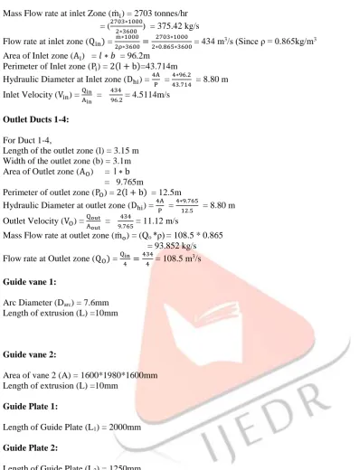
6.Geometrical calculation of 3D model duct Inlet Duct
IJEDR1803080
International Journal of Engineering Development and Research (
www.ijedr.org
)
469
Mass Flow rate at inlet Zone (ṁi) = 2703 tonnes/hr= (2703∗1000
2∗3600 ) = 375.42 kg/s Flow rate at inlet zone (Qin) = ṁ∗1000
2ρ∗3600=
2703∗1000
2∗0.865∗3600 = 434 m
3/s (Since ρ = 0.865kg/m3 Area of Inlet zone (Ai) = 𝑙 ∗ 𝑏 = 96.2m
Perimeter of Inlet zone (Pi) = 2(l + b)=43.714m Hydraulic Diameter at Inlet zone (Dhi) = 4A
P = 4∗96.2
43.714 = 8.80 m Inlet Velocity (Vin) =
Qin Ain =
434
96.2 = 4.5114m/s
Outlet Ducts 1-4:
For Duct 1-4,
Length of the outlet zone (l) = 3.15 m Width of the outlet zone (b) = 3.1m Area of Outlet zone (AO) = l ∗ b = 9.765m
Perimeter of outlet zone (PO) = 2(l + b) = 12.5m Hydraulic Diameter at outlet zone (Dhi) =
4A P =
4∗9.765
12.5 = 8.80 m Outlet Velocity (VO) =
Qout Aout =
434
9.765 = 11.12 m/s
Mass Flow rate at outlet zone (ṁo) = (Qo *ρ) = 108.5 * 0.865 = 93.852 kg/s Flow rate at Outlet zone (QO) = Qin
4 =
434
4 = 108.5 m 3/s
Guide vane 1:
Arc Diameter (Darc) = 7.6mm Length of extrusion (L) =10mm
Guide vane 2:
Area of vane 2 (A) = 1600*1980*1600mm Length of extrusion (L) =10mm
Guide Plate 1:
Length of Guide Plate (L1) = 2000mm
Guide Plate 2:
Length of Guide Plate (L2) = 1250mm
Guide Plate 3:
Length of Guide Plate (L3) = 2250mm
7.Mesh Generation and Boundary Conditions
Due to the symmetry in geometry, full 3D model ducts are considered for simulation. It contains 3 cases viz., Duct without guide vanes, with guide vanes, with guide plates. The meshing has been done in a GAMBIT 2.4.6 by setting as 150mm size of edges and 300mm size of faces and volume in Fig 1. Later on the Meshing has been exported to the ANSYS FLUENT 14 as Mesh and the scaling has been done from millimetre to meter. The mesh has been displayed by setting the edges in mesh section and outline as edge type as outline for visibility of Inlet parts. In models k-ε turbulence equation has been set for viscous effects. Due to the use of flue gas as working media, the properties of flue gas has been set such as ρ=0.865kg/m3, µ=2.145 x 10e-5kg/m-s. The name of material is set as Flue ga10e-5kg/m-s. The boundary conditions are set in the fluent as shown in Table 1.
Table 1 BOUNDARY CONDITIONS FOR DUCTING SYSTEM
Inlet Velocity – inlet
IJEDR1803080
International Journal of Engineering Development and Research (
www.ijedr.org
)
470
Symmetry Symmetry
Guide Vanes Wall
Guide Plate Wall
The velocity is set as 4.5m/s for inlet zone. The hydraulic diameter for inlet zone as 8.8m. The pressure at outlet is set as 0 Pa and its hydraulic diameter is 3.12m.
Fig 7 Meshing of 3D duct in Gambit
In Solution method, the scheme of Semi-Implicit Method for pressure linked Equations (SIMPLE) is followed for pressure velocity coupling gradient is set as Least Square Cell based. Pressure is set as Standard Pressure and momentum is set as Second Order Upwind because of its combination of accuracy and stability which interpolates the variable on the surface of the control volume. The scale of residuals has been set as 1e-03 for continuity, momentum and turbulence quantities. The solution has been initialized by setting compute from all zones. The calculations has been done by running for 100 iterations for initial results and 1000 iterations for Convergence results. The iso-surfaces has been created as: x-4.625, y-7.87, z-11.3 for viewing Pressure and velocity counters. Same procedure has been set for three iterations for making equal flow of a flue gas in outlets. The results for pressure and velocity has been computed.
8. Analysis of Velocity Zones:
The high velocity zone has been analysed by setting zone velocity from 18m/s to 30m/s. The low velocity zones has been analysed by setting velocity from 0 to 4m/s. In high velocity zones, there is some erosion occurs due to high pressure flow o f hot flue gas or ash will flow to atmosphere. In low velocity zones, Ash will deposit in the ducts.
9.RESULTS AND DISCUSSION
Now the pressure and velocity contours along with percentage deviations of mass flow rate, Average pressure and velocity has been analysed for five cases including Base case, Base case with guide vanes and Guide Plate Varying the angles.
9.1 Actual duct System
Figure 8 and Figure 9 shows the contours of Static Pressure and static velocity for the proposed duct. The pressure is increased at inlet when the coal is dropped and it gradually decreases when it becomes ash and flue gas at outlet. The velocity is lower at the inlet and it gradually increases at outlet according to flow of flue gas. This shows the flow is maximum in all zones due to equal supply of flow in outlet ducts.
IJEDR1803080
International Journal of Engineering Development and Research (
www.ijedr.org
)
471
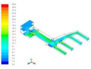
Fig 9. Contours of Velocity magnitude for base ductFigure 10 and Figure 11 shows high velocity zones and low velocity zones for base duct. The high velocity zones are formed in the corners of duct from inlet zone and to the entry of outlet zones. This is the cause of erosion occurs in the duct due to high pressure. This is the cause of erosion occurs in the duct due to high pressure. Low velocity zones are formed due to deposition of ash in the ducts at low velocity inlet and symmetry zones and slightly in outlet zones.
The high velocity zones has been set from 18m/s to 30m/s because after 25m/s the duct gets eroded. The low velocity zones has been set because there is chance of ash deposition and also the flue gas may flow slowly.
Fig 10. High velocity zones in Base duct
Fig 11. Low Velocity Zones in Base duct
9.2 Ducting System with Guide vanes
IJEDR1803080
International Journal of Engineering Development and Research (
www.ijedr.org
)
472
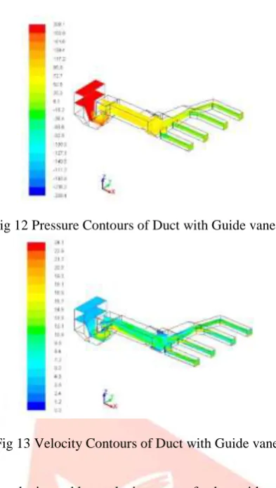
Fig 12 Pressure Contours of Duct with Guide vanes
Fig 13 Velocity Contours of Duct with Guide vane
Figure 14 and Figure 15 shows the high velocity and low velocity zones of a duct with guide vanes. The high velocity zones are occurs in the corners of the guide vanes and also in between the inlet and flow path of the ducts and also appears more in outlet zone corners. Guide vanes are applied for prevention of erosion in walls of ducts. In Low velocity zone, ash may deposit in inlet zone, on the guide vanes and outlet zones. The flue gases are deposited from of the ducts inlet to outlet through flow branches and also in symmetry. The flow is supplied equally to outlet planes by placing guide vanes.
Fig 14 High Velocity Zones of duct with guide vanes
Fig 15 Low Velocity Zones of duct with guide vanes
9.3 Ducting System with Guide Plate according to angle variation by NG method
IJEDR1803080
International Journal of Engineering Development and Research (
www.ijedr.org
)
473
The velocity is less in the inlet zone and slightly increases in the outlet zone. The equal flow of flue gas in four outlet pipes is set by attachment of guide vanes and also chamfering at the branch near the inlet zone. The flow of flue gas is obstructed by placing guide vanes. So, the flue gas is supplied equally in 4 outlet ducts.Fig 16 Pressure Contours of Duct with Guide Plate at the angles Ө1=45°, Ө2 =135°, Ө3=155°
Fig 17 Velocity Contours of Duct with Guide Plate at the angles Ө1=45°, Ө2 =135°, Ө3=155°
The arise of high velocity and low velocity zones has shown in Fig 16 and Fig 17. In high velocity zones the erosion has stopped to occur by placing a guide Plates according to angle variation whereas in low velocity zones the flow of flue gas is equal in all zones.
Fig 18 High Velocity Zone at the angles Ө1=45°, Ө2 =135°, Ө3=155° Fig 19 Low Velocity Zone at the angles Ө1=45°, Ө2 =135°, Ө3=155°
IJEDR1803080
International Journal of Engineering Development and Research (
www.ijedr.org
)
474
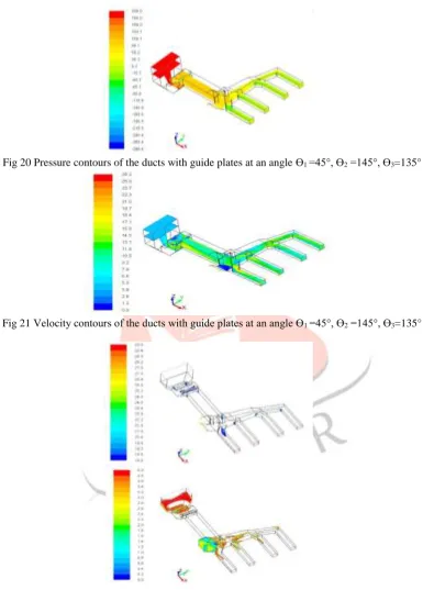
The same has been occurred in the pressure and velocity contours of the ducts with guide plates at an angle Ө1=60°, Ө2 =145°, Ө3=135° which is shown in Fig 24 and Fig 25. So, the maximum flow of flue gas to outlet zone 1, 2 and minimum in Outlet zone 3, 4 by varying angles.Fig 20 Pressure contours of the ducts with guide plates at an angle Ө1=45°, Ө2 =145°, Ө3=135°
Fig 21 Velocity contours of the ducts with guide plates at an angle Ө1=45°, Ө2 =145°, Ө3=135°
Fig 22 High Velocity Zone with guide plates at an angle Ө1=45°, Ө2 =145°, Ө3=135° Fig 23 Low velocity zone with guide plates at an
angle Ө1=45°, Ө2 =145°, Ө3=135°
IJEDR1803080
International Journal of Engineering Development and Research (
www.ijedr.org
)
475
Fig 24 Pressure contours of the ducts with guide Plate at an angle Ө1=60°, Ө2 =145°, Ө3=135° Fig 25 Velocity contours of the ducts with guide plates at an angle Ө1=60°,Ө2 =145°, Ө3=135°
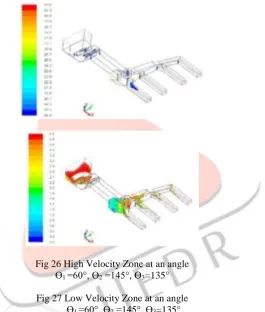
The same has been occurs in high velocity and low velocity zones of duct with guide plate at their angles Ө1=60°, Ө2 =145°, Ө3=135° which is shown in Fig 26 and Fig 27.
Fig 26 High Velocity Zone at an angle Ө1=60°, Ө2 =145°, Ө3=135°
Fig 27 Low Velocity Zone at an angle Ө1=60°, Ө2 =145°, Ө3=135°
9.4 Analysis of Variation in Percentage Deviation of Mass flow rate
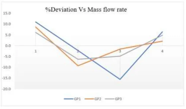
The Table 2 shows the variation of % deviation in mass flow rate. There is a progressive reduction in all streams in case of base case without GV, case with guide vanes and guide plate shows improvement due to optimization. The angle simulation of these three cases has been done using NG method. Negative deviation in mass flow rate occurs because it is less than average Mass flow rate of the Outlet zone whereas Positive deviation occurs because it is higher than average mass Flow rate in Outlet Zone. Square deviation error in Percentage deviation in Base case without Guide Vane is more than all other cases.
IJEDR1803080
International Journal of Engineering Development and Research (
www.ijedr.org
)
477
Fig 28 Graph of Percentage deviation Vs Mass flow rate9.5 Analysis of Variation in Pressure Drop
Figure 29 shows the variation of Pressure drop in all zones such as inlet and outlet zones 1-4. In the inlet zone, Pressure drop increases according to all the cases. The pressure at the inlet zone in GP 3 duct is slightly increased when compared to all other cases as uniformly comes with increase in pressure drop due to optimization but in outlet zones the pressure is obtained as zero due to equal flow.
Fig 29 Graph of variation in Pressure drop
In Table 3 same as in Fig 29, the inlet pressure is increased in the base case (duct) without guide vanes increases rather than the other cases and also the pressure drop raises the same.
Table 3 ANALYSIS OF PRESSURE DROP IN EACH ZONE Vs EACH CASES
IJEDR1803080
International Journal of Engineering Development and Research (
www.ijedr.org
)
478
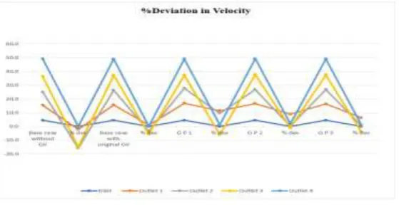
Fig 30 shows the Graphical comparison of % deviation of velocity in each cases. There is a progressive reduction in % deviation in all cases and velocity increases.Fig 30 Graph of Percentage deviation in Average velocity
The variation of velocity and its deviation is shown in the Table 4. Here, the deviation of velocity in each cases contains negative values. Negative deviation in velocity occurs because it is less than average velocity of the Outlet zone whereas Positive deviation occurs because it is higher than average velocity in Outlet Zone. Square deviation error in Percentage deviation in Base case without Guide Vane is more than all other cases.
Table 4 ANALYSIS OF PERCENTAGE DEVIATION IN VELOCITY
9.7 Analysis of Percentage Deviation in flow rates in ESP streams
Fig 4. shows graphical comparison of % deviation of flow rates in ESP streams. This shows the deviations in outlet zones 1-4 with the cases of angle variation of guide plates.
Fig 25 Graph of Percentage deviation of flow rates in ESP streams
IJEDR1803080
International Journal of Engineering Development and Research (
www.ijedr.org
)
479
In outlet zones for three cases of Guide plate angle variation, the deviation of flow increases at the positive values along with comparison of outlet deviations of duct along with angle varied Guide Plates is shown in Table 5. In outlet zones for three cases of Guide plate angle variation, the deviation of flow increases at the positive values. The deviation of outlet 1 increases than the outlet 4 whereas the % deviation of outlet 2 and 3 decreases. The Outlet 2 and 3 has negative values and outlet 1-and 4 has positive values. Hence all the above cases showing improvement due to optimization.10.CONCLUSION
The layout optimization for ducting between air preheater and Electrostatic precipitator has been analyzed using CFD. The equal flow has been supplied within the deviation of ±10% after using guide vanes and guide plates (GP3 case).The numerical computations is done by applying Continuity, Momentum, Energy and k-ε turbulence kinetic energy equations at discretized zones of the domain. The uniform flow across a cross section has been made and excess velocity, very low velocity and has been removed by placing guide vanes. The pressure drop in the duct between Air Pre-Heater and Electro-Static Precipitator (ESP) has been calculated. The Percentage deviation of mass flow rate, Average velocity Flow rate in ESP Streams are also analysed.
Acknowledgement
The author would like to thank Senior manager, Employees and Apprentice students of Layouts (RPD)/PE (FB)), BHEL, Trichy to carry out this project in Layouts department.
REFERENCES
[1] V.B.Gawande, Dr. D.B. Zodpe, G.P.Pawar, “Flow analysis of flue gases in ESP inlet duct using CFD”, Proc. of the 4th International Conference on Advances in Mechanical Engineering, September 23-25, 2010 S.V. National Institute of Technology, Surat – 395 007, Gujarat, India.
[2] Shah M.E. Haque , M.G. Rasul , M.M.K. Khan , A.V. Deev , N. Subaschandar, “Influence of the inlet velocity profiles on the prediction of velocity distribution inside an electrostatic precipitator”, Experimental Thermal and Fluid Science 33 (2009) 322–328.
[3] Shah M.E. Haque , M.G. Rasul , A.V. Deev , M.M.K. Khan , N. Subaschandar “Flow simulation in an electrostatic precipitator of a thermal power plant”, Applied Thermal Engineering 29 (2009) 2037–2042.
[4] Laszlo C1zetany, Zoltan Szantho, Peter Lang, “Modelling of the in-duct sorbent injection process for flue gas desulfurization” Separation and Purification Technology 62 (2008) 571–581.
[5] Ramesh Avvari, Sreenivas Jayanti, “Flow apportionment algorithm for optimization of power plant ducting”, Applied Thermal Engineering 94 (2016) 715–726.
[6] Ramesh Avvari, Sreenivas Jayanthi, “Heuristic shape optimization of gas ducting in process and power plants” Chemical Engineering research and design 91 (2013) 999-1008.
[7] C. Bhasker, “Flow simulation in Electro-Static-Precipitator (ESP) ducts with turning vanes” Advances in Engineering Software 42 (2011) 501–512.
[8] A.S.M.Sayema, M.M.K. Khana, M.G. Rasula, M.T.O. Amanullahb, N.M.S.Hassan “Effects of baffles on flow distribution in an electrostatic precipitator (ESP) of a coal based power plant”, Journal of Procedia Engineering 105 ( 2015 ) 529 – 536.
[9] Madhulika Singh, Shah Alam, “CFD Approach to Design and Optimization of Air, Flue Gas Ducting System”, International Journal of Advance Engineering and Research Development Volume 2, Issue 5, May -2015.
[10]Luca Marocco, Alessandro Mora, “CFD modelling of the Dry-Sorbent-Injection process for flue gas desulfurization using hydrated lime”, Separation and Purification Technology 108 (2013) 205–214.
[11]Laszlo Czetany , Zoltan Szantho, Peter Lang, “Rectangular supply ducts with varying cross section providing uniform air distribution”, Applied Thermal Engineering 115 (2017) 141–151.
IJEDR1803080
International Journal of Engineering Development and Research (
www.ijedr.org
)
480
[13]Bhutta M. M. A., Nasir H., Bashir M. H., Khan A. R., Ahmad K. N., Khan S., “CFD applications in various heatexchangers design”: A review Article, Applied Thermal Engineering, volume 32, Pages 1-12, January 2012.
[14]Halil Bayram , Gokhan Sevilgen, “Numerical Investigation of the Effect of Variable Baffle Spacing on the Thermal Performance of a Shell and Tube Heat Exchanger”, Journal on energies 2017, 10,1156.
[15]Z. Duan, M.M. Yovanovich, Y.S. Muzychka, “Pressure drop for fully developed turbulent flow in circular and noncircular ducts”, J. Fluids Eng. 134 (6) (2012).
[16]Y.S.Chen, S.W.Kin, “Computation of Turbulent Flows Using an Extended k-s Turbulence Closure Model”, Journal of University Space Research Association under NASA Contract NAS8-35918,1987 .
[17] H. Liu, P. Li, J.V. Lew, “CFD study of flow distribution uniformity in fuel distributors having multiple structural bifurcations of flow channels”, Int. J. Hydrogen Energy 35 (2010) 9186–9198.
[18]J.C.K. Tong, E.M. Sparrow, J.P. Abraham, “CFD Simulation for Manifold with Tapered longitudinal Section”, International Journal of Emerging Technology and Advanced Engineering (ISSN 2250-2459,ISO 9001:2008Certified Journal, Volume 4, Issue 2, February 2014).
[19]M. M. Matheswaran, S. Karthikeyan, N. Rajiv Kumar2, “Flow distribution of Heat exchanger with different header configuration”, ARPN Journal of Engineering and Applied Sciences VOL. 11, NO. 5, 2016, ISSN 1819-6608. [20]Limin Wang, Yilin Fan, Lingai Luo, “Heuristic optimality criterion algorithm for shape design of fluid flow” Journal