Using Computer Techniques To Predict OPEC Oil
Prices For Period 2000 To 2015 By Time-Series
Methods
Mohammad Esmail Ahmad, Ali Jalal Hussian, Monem A. Mohammed
Abstract: The instability in the world (and OPEC) oil process results from many factors through a long time. The problems can be summarized as that the oil exports don’t constitute a large share of N.I. only, but it also makes up most of the saving of the oil states. The oil prices affect their market through the interaction of supply and demand forces of oil. The research hypothesis states that the movement of oil prices caused shocks, crises, and economic problems. These shocks happen due to changes in oil prices need to make a prediction within the framework of economic planning in a short run period in order to avoid shocks through using computer techniques by time series models.
Keywords: Fluctuations in oil prices, prediction, Time-Series Forecasting, computer techniques, Holt Winter, Exponential Smoothing, Analyzing Techniques, Stationary, information technology.
————————————————————
INTRODUCTION
Oil is important for the entire world, so it doesn’t play as good as a vital role in economic life as the oil play in underdeveloped countries. Clearly, oil is the economic life for countries that have oil, such as Venezuela, Middle East, Arabian Gulf and North Africa. Oil exports do not constitute a large share of national income only. Also, it makes up most of the saving of the oil states. Therefore, Oil is the primary Source of capital needed for economic development. Also, Oil as fuel is indispensable for modern agriculture and industry sector in addition to being a major fuel meets needs to secure the necessary consumption. So we can summarize importance of Oil and the role in the following properties: [2]
1. It could be considered as a key driver of the global economy.
2. It could be considered as a major or source of energy within the global economy.
3. It could be considered as more strategic goods traded. 4. It significantly contributes to the G.D.P of
under-developed countries.
5. It significantly contributes to the government revenues of underdeveloped countries.
6. It significantly contributes to the balance of payments of underdeveloped countries.
7. It can contribute to creating interdependence between industry, agriculture, and services.
1.1 The Research Problem:
Can be summarized as that oil prices affect their market through the interaction of supply and demand forces of oil according to tracker for evolution of oil prices to historic periods of times characterized by large and volatile swings, sometimes up and down movement due to upward and downward economic activity for global economy between stagnation and growth, which is reflects positively or negatively impact on prices.
1.2 The Research Hypothesis:
The research hypothesis states:
―The movement of oil prices (downward and upward) caused shocks, crises, and economic problems.‖ These shocks happen due to changes in oil prices need to make forecasts within the framework of economic planning in a short run period in order to avoid shocks.
1.3 The Research Importance:
Time-Series is one of the most important predictive methods in short-run term because of its importance in the field of economic planning in general and in particular of prices. The researchers resorted to use computer techniques (Microsoft Excel, Statistical Analysis Software Package-SPSS) and forecasting method (Time-series), in addition to the analytical method for analyzing the reality of oil prices in the period of research.
1. THEORETICALFRAMEWORK
The importance of forecasting in economics field had been expanded due to increasing of economic problems, it make adoption of economic planning to avoid these problems. It came when economic fluctuation happened to avoid losses in potential resources. The forecasting conducts demands and prices to make the possibility to apply economic policies in order to affect demands and prices in different levels. So predictability needs to increase using economic indicators such as price elasticity to make policies in order to overcome problems. The evolution in the field of computer and information systems generate accuracy of predictions. [11]
_____________________
Assis. Lect. Mohammad Esmail Ahmad is a lecturer at University of Sulaimani, M.Sc. in the field of Computer Science, E-mail: [email protected]
Assis. Prof. Dr. Ali Jalal Hussian is a lecturer at University of Sulaimani, PhD in the field of Economics, E-mail: [email protected]
2.1 The Stages of Forecasting:
The prediction process doing through following stages: [1] 1. Building model: It makes through building model. 2. Estimating model: It makes that building model to find
the data for economic variables in the models, and choice the relevance method for estimating according to computer requirement and prediction specification. 3. Evaluate model: It makes building model to analyze the
economic indicators from where the sign and value of estimated coefficient within the framework of economic theory.
4. Preparing forecasts through using data accurate predictions.
2.2 Forecasting Methods:
There are different methods and techniques for forecasting according to the different level of complexity, the theoretical foundations, and Statistical requirement. So the methods used vary about the accuracy of forecasts. The major technique for forecasting is time-series. It’s interested in analyzing the time – trend of the economic phenomenon to be predictable. Forecasting is very important for prediction of the feature events .Science and computer technology together has made significant advances over the past several years and using those advanced technologies and few past patterns, it grows the ability to predict the future .Feature prediction is a process of choosing the best subset of the features available from the selected input data .The best subset contains the minimum number of dimensions that contribute more accuracy. [12]
2.3 Time Series Model:
Some models such as the Oil pricing model and the arbitrage pricing model described as time series data. However, there is much to be said for analyzing data without imposing constraints that are implied by a theory. The aim of time series analysis is to find the most appropriate statistical model for the data and to use this model for prediction. In this way, the variables are allowed to speak for themselves. Without the confine of economic theories. In Oil markets, the modelling procedures for return data and for price data are different to understand why. On needs to draw the basic distinction between stationary and non-stationary time series Daily and Monthly return data on most Oil markets are generated by stationary processes and consequently returns. In fact, they are often rapidly mean-reverting since there is very little autocorrelation in many oil market returns. The statistical concepts and methods that apply to return data do not apply to price data. For example volatility and correlation are concepts that only apply to stationary processes it makes no sense to try to estimate volatility or correlation on price data. Daily (log) price data are commonly assumed to be generated by a non-stationary stochastic process. [7]
2.4 Concept of Information Technology:
Human started from ancient to think about how to arrange their works with methods that guarantee them the best use of time and effort, with the appearance of computerized machines which have had a significant role in the conduct of business, and gradually the computer programmer emerged, causing a growth in all aspects of scientific, technical and administrative life as it began this
renaissance leading investment into the world of technology.The term Information Technology (IT) has appeared in the early seventies with the emergence of electronic computer on a commercial scale, and the concept of information technology means all the things that include computers of various types and data processing in all its forms and information and all the centers and functions related to technology and services in organizations and institutions, as well as software and programming packages that are used in doing business, jobs, and product marketing. [8] ―Information Technology (IT) may be defined as the technology that is used to acquire, store, organize, process, and disseminate processed data which can be used in specified applications. Information is processed data that improves our knowledge, enabling us to take decisions and initiate actions‖. [13]
2.5 Importance of Information Technology:
The Importance of (IT) can be summarized as the following: [16]
1. Information Technology works on major changes in the entire organization, as in their products, markets, and gives employees the flexibility to work anywhere either in their organizations or at home.
2. Provide more information to assist controlling the decisions taken by their users.
3. Help to create new communication channels, therefore, it increases flowing, processing and exchanging information and develop modern management methods.
4. Works to improve and increase business opportunities between organizations, and between organizations and the government, which led to a wider spread of information.
5. Helps detecting deviations to prevent the aggravation and work on a specialized processor.
6. Helps to improve customer service by meeting their demands via terminals.
7. Improves the quality of work through the adoption of new technological methods and thus achieve high accuracy, shorten the time, reduce costs and risk of humanitarian unprepared interpretation of the information and data.
8. Contributes to reduce the volume of the costs which allocated to provide factors of production.
9. Improves the process of collecting, processing, storing, retrieving, updating and reducing cost of data as it would reduce the cost of administrative work.
10. Creating the most effective managerial tools to apply what can be applied in the normal conditions and leading the renewal process.
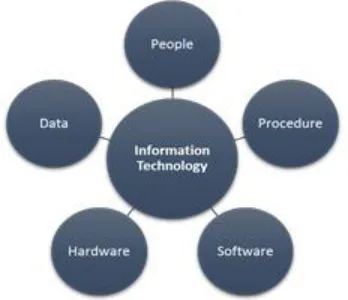
2.6 Component of Information Technology:
Fig. 1: Component of Information Technology
1. People: The most important part as they make
end-users more productive.
2. Procedure: Refer to rules or guidelines people follow
when using software, hardware, and data. Documented in manuals written by computer specialists and provided by software/hardware manufacturers of the product.
3. Software: It is the term for programs or sets of
computer instructions written in a special computer language that enables a computer to accomplish a given task. It consists of step-by-step instructions, which the computer can use to convert data into information.
4. Hardware: Refers to physical, touchable pieces or equipment.
5. Data: Raw, unprocessed facts including text, numbers,
images and sounds. Data describes something that is stored electronically in a file.
2.7 Statistics by MS-Excel:
There are a number of commonly used, powerful tools for carrying out statistical analyses. The most popular of these are Statistical Package for the Social Sciences (SPSS), Statistical Analysis System (SAS), Stata, Minitab and R. Many researchers choose to apply Excel as their major analysis tool or as a complementary to each other tools for any of the following reasons: [19]
1. It is widely available and so many researchers already know how to use it.
2. It is not necessary to pay the cost of another tool (as some of the popular tools are quite expensive).
3. It is not necessary to learn new methods of manipulating data and drawing graphs.
4. It provides numerous built-in statistical functions and data analysis tools.
5. It is much easier to see what is going on since, unlike the more commonly used statistical analysis tools, very little is hidden from the user.
6. It provides the user with a lot of control and flexibility.
2.8. Techniques Used:
2.8.1 Moving Average:
The moving averages method uses the average of the most recent k data values in the time series as the forecast for
the next period. Mathematically, a moving average forecast of order k is as follows: [5]
𝐹 =∑ =
(1)
Where;
𝐹 = 𝑓𝑜𝑟𝑒𝑐𝑎𝑠𝑡 𝑜𝑓 𝑡𝑒 𝑡𝑖𝑚𝑒𝑠 𝑠𝑒𝑟𝑖𝑒𝑠 𝑓𝑜𝑟 𝑝𝑒𝑟𝑖𝑜𝑑 𝑡
+ 1
𝑌 = 𝑎𝑐𝑡𝑢𝑎𝑙 𝑣𝑎𝑙𝑢𝑒 𝑜𝑓 𝑡𝑒 𝑡𝑖𝑚𝑒 𝑠𝑒𝑖𝑟𝑒𝑠 𝑖𝑛 𝑝𝑒𝑟𝑖𝑜𝑑 𝑡
The term moving is used because every time a new observation becomes available for the time series, it replaces the oldest observation in the equation and a new average is computed. As a result, the average will change, or move, as new observations become available.
2.8.2 Exponential Smoothing:
Exponential smoothing uses a weighted average of past time series values as a forecast; it is a special case of the weighted moving averages method in which we select only one weight—the weight for the most recent observation. The weights for the other data values are computed automatically and become smaller as the observations move farther into the past. The exponential smoothing equation follows: [6]
𝐹 = 𝛼𝑌 + 1 − 𝛼 𝐹 (2)
Where;
𝐹 = 𝑓𝑜𝑟𝑒𝑐𝑎𝑠𝑡 𝑜𝑓 𝑡𝑒 𝑡𝑖𝑚𝑒 𝑠𝑒𝑟𝑖𝑒𝑠 𝑓𝑜𝑟 𝑝𝑒𝑟𝑖𝑜𝑑 𝑡 + 1
𝑌 = 𝑎𝑐𝑡𝑢𝑎𝑙 𝑣𝑎𝑙𝑢𝑒 𝑜𝑓 𝑡𝑒 𝑡𝑖𝑚𝑒 𝑠𝑒𝑟𝑖𝑒𝑠 𝑖𝑛 𝑝𝑒𝑟𝑖𝑜𝑑 𝑡 𝐹 = 𝑓𝑜𝑟𝑒𝑐𝑎𝑠𝑡 𝑜𝑓 𝑡𝑒 𝑡𝑖𝑚𝑒 𝑠𝑒𝑟𝑖𝑒𝑠 𝑓𝑜𝑟 𝑝𝑒𝑟𝑖𝑜𝑑 𝑡 𝛼 = 𝑠𝑚𝑜𝑜𝑡𝑖𝑛𝑔 𝑐𝑜𝑛𝑠𝑡𝑎𝑛𝑡 0 ≤ 𝛼 ≤ 1
2.8.3 Double Exponential Smoothing:
Charles Holt developed a version of exponential smoothing that can be used to forecast a time series with a linear trend. The smoothing constant α to ―smooth out‖ the randomness or irregular fluctuations in a time series; and, forecasts for time period t + 1 are obtained using the equation: [6]
𝐹 = 𝐿 + 𝐵 𝐾 + 𝜖 (3)
Forecasts for Holt’s linear exponential smoothing method are obtained using two smoothing constants, α and _, and three equations:
𝐿̂ = 𝛼𝑌 + 1 − 𝛼 𝐿̂ + 𝐵̂ (4)
𝑏̂ = 𝛽(𝐿̂ − 𝐿̂ ) + 1 − 𝛽 𝑏̂ (5)
𝐹 = 𝐿̂ + 𝑏̂𝑘 (K=1,2,…,n) (6)
Where;
𝐿 = 𝑒𝑠𝑡𝑖𝑚𝑎𝑡𝑒 𝑜𝑓 𝑡𝑒 𝑙𝑒𝑣𝑒𝑙 𝑜𝑓 𝑡𝑒 𝑡𝑖𝑚𝑒 𝑠𝑒𝑟𝑖𝑒𝑠 𝑖𝑛 𝑝𝑒𝑟𝑖𝑜𝑑 𝑡 𝑏 = 𝑒𝑠𝑡𝑖𝑚𝑎𝑡𝑒 𝑜𝑓 𝑡𝑒 𝑠𝑙𝑜𝑝𝑒 𝑜𝑓 𝑡𝑒 𝑡𝑖𝑚𝑒 𝑠𝑒𝑟𝑖𝑒𝑠 𝑖𝑛 𝑝𝑒𝑟𝑖𝑜𝑑 𝑡 𝛼 = 𝑠𝑚𝑜𝑜𝑡𝑖𝑛𝑔 𝑐𝑜𝑛𝑠𝑡𝑎𝑛𝑡 𝑓𝑜𝑟 𝑡𝑒 𝑙𝑒𝑣𝑒𝑙 𝑜𝑓 𝑡𝑒 𝑡𝑖𝑚𝑒 𝑠𝑒𝑟𝑖𝑒𝑠 𝛽 = 𝑠𝑚𝑜𝑜𝑡𝑖𝑛𝑔 𝑐𝑜𝑛𝑠𝑡𝑎𝑛𝑡 𝑓𝑜𝑟 𝑡𝑒 𝑠𝑙𝑜𝑝𝑒 𝑜𝑓 𝑡𝑒 𝑡𝑖𝑚𝑒 𝑠𝑒𝑟𝑖𝑒𝑠 𝐹 = 𝑓𝑜𝑟𝑒𝑐𝑎𝑠𝑡 𝑓𝑜𝑟 𝑘 𝑝𝑒𝑟𝑖𝑜𝑑𝑠 𝑎𝑒𝑎𝑑
2.8.4 Holt-Winters: (Triple exponential smoothing):
Holt (1957) and Winters (1960) extended Holt’s method to capture seasonality. The Holt-Winters seasonal method comprises the forecast equation and three smoothing equations—one for the level ℓ, one for trend 𝑏, and one for the seasonal component denoted by 𝑆, with smoothing parameters 𝛼, 𝛽 and 𝛾. We use 𝑚 to denote the period of the seasonality, i.e., the number of seasons in a year. There are two variations to this method that differ in the nature of the seasonal component. The additive method is preferred when the seasonal variations are roughly constant through the series, while the multiplicative method is preferred when the seasonal variations are changing proportionally to the level of the series. With the additive method, the seasonal component is expressed in absolute terms in the scale of the observed series, and in the level equation, the series is seasonally adjusted by subtracting the seasonal component. Within each year, the seasonal component will add up to approximately zero. With the multiplicative method, the seasonal component is expressed in relative terms (percentages) and the series is seasonally adjusted by dividing through by the seasonal component. Within each year, the seasonal component will sum up to approximately. [22]
It contains three equations: [11]
𝑆 = + 1 − 𝑎 {𝑆 + 𝑏̂ } (7)
for t= (1,2,..,n) and L=12
General Preliminary Exponential Equation
𝑏 = 𝛾 𝑠 − 𝑠 + 1 − 𝛾 𝑏 (8)
for t=(1,2,..,n) and L= 4
Time-Trend Preliminary Equation
𝐼 = + 1 − 𝛽 𝑖 (9)
for t= (1,2,..,n)
Seasonal Preliminary Equation
From the three equations above, we get the following Preliminary Exponential Tripartitly equation:
𝑍 = {𝑆 + 𝑏̂ 𝑚 }𝐼 (10)
for m=(1,2,…)
2.9 Stationary Time Series:
Let, we have stationary time series {𝑍; 𝑡 = 0 ± ,1 ± 2, … }, then, we have the following ARMA (P, q) process: [18]
𝑍 = ∅𝑍 + ∅ 𝑍 + + ∅ 𝑍 + 𝛼 − 𝜃 𝛼 −
𝜃 𝛼 − . . . −𝜃 𝛼 (11)
Where 𝑍= 𝑍̃ – μ
For each (t), (μ) is the mean of time series and {𝑎 }is a purely random error (white noise) distributed Gaussian with E (𝜕)= 0,
Variance of (𝜕)= E (𝜕)2 =𝜎 and
Covariance of (𝜕 , 𝜕 ± ) = 0, for all k ≠ 0.
Then, ARMA (1, 1) distributed Gaussian or normal distribution.
By using (𝐵) operator we get:
𝑍{1 − ∅ 𝐵 − ∅ 𝐵 −. . . −∅ 𝐵 }
= {1 − 𝜃𝐵 − 𝜃 𝐵 − − 𝜃 𝐵 } 𝑎 ∴𝑍 = { ∅{ ∅ ... ∅ }}𝑎 (12)
{ 𝑍 = 𝑎 } Where 𝛩 𝐵 𝑎𝑛𝑑 𝛷 𝐵 are the polynomial functions of order (q) and (p) in (B) respectively.
𝑜𝑟 { 𝑍 = 𝜓 𝐵 𝑎} where:
𝜓 𝐵 = = 𝜓 𝐵 + 𝜓 𝐵 + 𝜓𝐵 + 𝜓 𝐵 + , 𝜓 = 1 (13)
𝜓 𝐵 = = ∑ 𝜓𝐵 , 𝜓 = 1 𝜓 = 1, 𝜓 , 𝜓 , ψ, … are the weights.
2.10 Autocorrelation Function of the Autoregressive Moving Average Model:
For St. Time series (𝑍 , (t = 1, 2, 3… n) [17]
𝑍 = ∅ 𝑍 +∅ 𝑍 + ....+ ∅ 𝑍 +𝑎 - 𝜃𝑎 - 𝜃 𝑎 -
... - 𝜃 𝑎 (14)
By using Yule – walker equations we get the (ACF) as follows:
Let the auto correlation with lag (k) is:
𝐸 𝑍. 𝑍 = ∅ 𝐸 𝑍 . 𝑍 + ∅ 𝐸 𝑍 . 𝑍 + +
∅ 𝐸 𝑍 . 𝑍 + 𝐸 𝑎. 𝑍 − 𝜃𝐸 𝑎 . 𝑍 −
𝜃 𝐸 𝑎 . 𝑍 − − 𝜃 𝐸 𝑎 . 𝑍 (15)
With (k = 0, 1, 2 ...), and by using covariance form with lag (k) is (𝑅 ) then, we have:
𝑅 = ∅𝑅 + ∅ 𝑅 + + ∅ 𝑅 + 𝐸 𝑎. 𝑍 −
𝜃 𝐸 𝑎 . 𝑍 − 𝜃𝐸 𝑎 . 𝑍 − − 𝜃 𝐸 𝑎 . 𝑍 (16)
Now, 𝐸 𝑎 . 𝑍 = 0 𝑓𝑜𝑟 𝑘 > 𝑡 .
So, 𝑅 = ∅ 𝑅 + ∅ 𝑅 + + ∅ 𝑅 , with (k ≥
q+1)
Let the (ACF) is: 𝜌 = , (k = 0 ± ,1 ± 2, … .
Then, 𝜌 = ∅𝜌 + ∅ 𝜌 + + ∅ 𝜌 with (k ≥
q+1)
∴ 𝜌 = ∑
∑ , (k = 0 ± ,1 ± 2, … (17)
For example: for AR(1) process we have: 𝜓 = ∅ , with |∅ | < 1
𝜌 = ∑
∑ =
∑ ∅∅ ∑ ∅
=
∅ ∅
∅
= ∅ , With (k
=0 ± ,1 ± 2, … .
2.11 The Partial Autocorrelation Function:
The autocorrelation function of an MA series exhibits different behavior from that of AR and general ARMA series. The (ACF) of an (MA) series cuts of sharply whereas those for (AR) and (ARMA) series exhibit exponential decay (with possible Sinusoidal behavior superimposed). This makes it possible to identify an (ARMA) series as being a purely (MA) one just by plotting its autocorrelation function. The partial autocorrelation function provides a similar way of identifying a series as a purely (AR) one. Given a stretch of time series values:
𝑍 , 𝑍 , … , 𝑍 , 𝑍, …
The partial correlation of (𝑍) and (𝑍 ) is the correlation
between these random variables which is not conveyed through the intervening values. If the (𝑍) values are normally distributed, the partial autocorrelation between (𝑍) and (𝑍 ) can be defined as the partial autocorrelation
function can be thought of as the partial regression coefficition ∅ in the representation: [14]
𝑍 = ∅ 𝑍 + ∅ 𝑍 + + ∅ 𝑍 + 𝑎
Where: ∅ ; 𝑖 = 1,2, … , 𝑘
Denoted the (i) regression parameters and (𝑎 ) is a
normal error term, uncorrelated with 𝑋 for 𝑗 ≥ 1 But
the additional correlation between (𝑍) and (𝑍 ) after their
mutual linear dependency on the intervening variables {𝑍 ,𝑍 ,… , 𝑍 ,} has been removed which is usually
followed by a conditional autocorrelation as:
∅ = Cor Z, Z |Z , … , Z
And after solving the equations of general formula to determining the initial estimates for parameters (∅ ) and
(∅ ) under the stationary condition we have: [11]
∅ , =
∑ ∅
∑ ∅ (18)
And
∅ , = ∅ − ∅ , ∅ , , (j=1, 2, ... k) (19)
3.
PRACTICAL
FRAMEWORK
In our research, we gather data of Oil basket price for the period of Jan 2000 to Feb 2016. We use different methods to predict the price for next 6 months with the help of computer system using Microsoft Excel and SPSS technology, then carried out a comparative study of nine different forecasting technique. The data set is used, was collected from the OPEC & OAPEC organization. [21]
3.1 Descriptive model:
The researchers used Microsoft Excel to estimate the following time series methods forecasting OPEC oil prices for period (2000-2015):
1. Time series moving average smoothing. 2. Time series exponential smoothing.
3. Time series Double exponential smoothing. 4. Time series Holt winter-(additive) model. 5. Time series Holt winter-(Multiplicative) model. 6. Time series Holt winter-(No Trend) model.
So the results shown in the bellow table:
Table 1: Time series model indicators:
Model M.S.E.
a 66.444
b 55.030
c 56.943
d 55.357
e 57.455
f 54.847
The above table shows that the mean squares error (M.S.E) indicates that the minimum value is (54.847) in spite of (Holt winter no-trend), but this value is still high level. We can show, in (Figure 2), the time plot of actual Vs. Forecast data as bellow.
Fig. 2: represent the actual price oil Vs. Forecast price oil
We conclude that the model above (f) suffer from Autocorrelation problem, because the estimators characterized by non-stationary estimators.
3.2 Box and Jenkins models analysis:
To analysis the data of (Oil-Price) by using (Box and Jenkins) models to show the problem of the data in time series, we can applied the following steps in order to overcome the problem by using SPSS system:
0 20 40 60 80 100 120 140
Jan-00 Sep-02 Jun-05 Mar-08 Dec-10 Sep-13 Jun-16
US
$/Ba
rre
l
months
Time Plot of Actual Vs. Forecast
Step (1): The actual Sequence Series plot:
Fig 3: represent the actual Sequence Series plot
Step (2): The (ACF and PACF) of actual sequence series Plots:
Fig. 4: represent the (ACF and PACF) of actual sequence series plot.
Fig. 5: represent the first difference of actual sequence series plot
Step (3): Take the first difference for Sequence series plot as follows:
Fig. 6: represent the first difference of actual sequence series plot
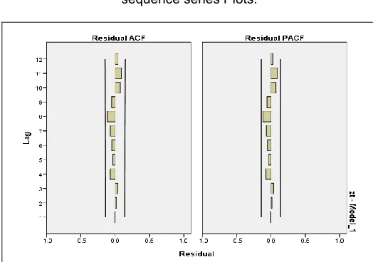
Step (4): The ACF and PACF of the first difference of sequence series Plots:
Fig. 7: represent the (ACF and PACF) of the first difference of sequence series plot
Step (5): From analysis all (Box and Jenkins) models, we consider the following (ARIMA) Models to forecasting the
(Oil –Prices) in year (2016):
Table 2: Represented the (ARIMA) models:
Models R-Square R MSE BIC
ARIMA(0,1,2) 0.949 7.350 4.072
ARIMA(2,1,2) 0.949 7.347 4.126
ARIMA(2,1,0) 0.949 7.368 4.077
ARIMA(2,1,1) 0.949 7.386 4.109
From above table we show that the best model is ARIMA (0, 1, 2) has the less values of (R MSE = 7.350, Bic = 4.072) and has the greatest (R- square = 0.949).
Table 3: Represent Forecasting (ARIMA) models in year (2016):
Models 193 194 195 196 197 198 199 200 ARIMA
(0,1,2) 33.
27 31. 87
31. 90
31. 94
31. 97
32. 00
32. 04
32. 07 ARIMA
(2,1,2) 32.
33 34. 01
35. 43
34. 28
33. 04
33. 91
35. 12
34. 62 ARIMA
(2,1,0) 33.
29 32. 20
32. 21
32. 06
32. 10
32. 10
32. 13
32. 16 ARIMA
(2,1,1) 33.
29 32. 14
32. 06
31. 89
31. 90
31. 90
31. 92
31. 95 From above table we show the range of predicted oil prices for (6) months, approximately between 31 $ to 33 $ for
barrel.
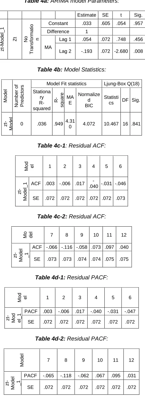
Table 4a: ARIMA model Parameters:
Table 4b: Model Statistics:
Mod
e
l
N
u
mbe
r
o
f
P
re
d
ic
to
rs Model Fit statistics Ljung-Box Q(18)
Stationa ry R-squared
R
-s
q
u
a
re
d
MA E
Normalize d BIC
Statisti
cs DF Sig.
zt
-Mod
e
l
_10 .036 .949 4.310 4.072 10.467 16 .841
Table 4c-1: Residual ACF:
Mod el 1 2 3 4 5 6
zt
-Mod
e
l_1 ACF .003 -.006 .017
-.040 -.031 -.046 SE .072 .072 .072 .072 .072 .073
Table 4c-2: Residual ACF:
Mo del 7 8 9 10 11 12
zt
-Mod
e
l
_1
ACF -.066 -.116 -.058 .073 .097 .040 SE .073 .073 .074 .074 .075 .075
Table 4d-1: Residual PACF:
Table 4d-2: Residual PACF:
Table 4e: Forecast:
For each model, forecasts start after the last non-missing in the range of the requested estimation period.
Fig. 8: Time plot of actual VS Forecast. ARIMA estimated model
From the figure above, we show that the actual values VS predicted values are very approach, which means the estimators are best and stationary.
4.
CONCLUSIONS
The researcher reaches to the following major conclusion: 1. The oil price was fluctuates through long-term period.
And it causes shocks, crises and many economic problems for OPEC countries.
2. The necessity of oil price in economies of oil generates to make prediction for oil prices in order to subjugate that in planning to avoid the economic problems. 3. The famous and the best method or forecasting is time
series, that it plays important role for this purpose. 4. The estimated model, (Moving average, exponential
smoothing, and Holt winter) suffer from Autocorrelation problem, so we must to overcome this problem. 5. By using (Box and Jenkins) models we proved that
ARIMA (0,1,2) is the best estimated model which become greater stationary and has less Mean squared Error (M.S.E).
6. The range predicted (oil –prices) of OPEC for next six months approximately between 31 $ to 33 $ for barrel. 7. Any change upper or down the range above is affected
by exogenous variables. Estimate SE t Sig.
zt
-Mod
e
l_1
Z
t
N
o
Tr
a
n
s
fo
rma
tio
n
Constant .033 .605 .054 .957 Difference 1
MA
Lag 1 .054 .072 .748 .456 Lag 2 -.193 .072 -2.680 .008
Mod el 1 2 3 4 5 6
zt
-Mod el_1
PACF .003 -.006 .017 -.040 -.031 -.047
SE .072 .072 .072 .072 .072 .072
Mod
e
l
7 8 9 10 11 12
zt
-Mod
e
l
_1
PACF -.065 -.118 -.062 .067 .095 .031 SE .072 .072 .072 .072 .072 .072
Mod
e
l
193 194 195 196 197 198 199 200
zt
-Mod
e
l_1 For
e
c
a
s
t
33.27 31.87 31.90 31.94 31.97 32.00 32.04 32.07
U C L47.77 51.83 57.81 62.66 66.85 70.60 74.01 77.18
5.
REFERENCES
5.1 Books and Researches:
[1] Abraham, B. and LEDOTER, J. 1983, ―Statistical methods for forecasting‖, Johan Wiley, NEWYORK.
[2] Al-HEETY, A., 2000, ―Economies of petrol, Mosel University Pub., Mosel (Arabic Reference).
[3] Al-MAZINI, E., 2013, ―The factors affect the fluctuations in world oil prices (2000-2010)‖, Al-AZHAR University Journal – Gaza, human sciences, vol. 15, Nov.
[4] Anderson, T.W, 1971, ―The statistical analysis of Time series, John Wiley, NEWYORK.
[5] Anderson, D., Sweeney, D., 2015, ―Modern Business statistic with Microsoft Excel‖, CENGAGE learning Pub., NEWYORK.
[6] Anderson, D., Sweeney, D., Williams, T., 2011, ―Statistics for Business and Economics‖, Eleventh Edition, CENGAGE Learning pub., NEWYORK.
[7] Box, G.E.P. and Jenkins, G.M., 1976, ―Time series analysis Forecasting and control, Holden-Day Inc., San Francisco.
[8] El-DABAGH, M., 2010, ―Design of Instant-Mail System using infrastructure of information and communication technology‖, Higher Diploma thesis, Mosul University – college of Administration and Economic, (Arabic Reference).
[9] ESMAEEL, N., 1981, ―Determine the Arabian Crude oil Prices in the world Market‖, AL-RASHID Pub., Baghdad (Arabic reference).
[10] JAWAD, B., 2013, ―Wide Preaching and Information Technology and their Impact on Achieving customers satisfaction‖, Master thesis, Karbala University – college of Administration and Economic, (Arabic Reference).
[11] MONEM M.A. 2011, ―The analysis and Forecasting in Time series‖, SULIMANI University Pub., SULIMANI. (Arabic reference).
[12] PADHY, N., and PANIGRAHI, R., 2012, ―Engineering information Technology, International Journal of computer, Vol.2, NO.5, Oct.
[13] RAJARAMAN, V., 2013, ―Introduction to Information Technology‖, second edition, PHI learning Private Limited.
[14] SIM, C.H., 1978, ―AMIXED GAMMA ARAMA (1, 1) Model for river flow Time Series‖, Water resources research, Vol.23, NO.1.
[15] SPYROS, M., Steven, C., and ROB, J., 1998, ―Forecasting methods and applications‖.
[16] SULTAN, S., 2005, ―Health information technology and its impact on job satisfaction – a study on opinions of sample of health technologies users in Ibn Sina & El-Khansa educational Hospital‖, Master thesis, University of
Mosul-[17] TSAY, R.S., and TIAO, G.C., 1948, ―Consistent estimates Autoregressive Parameters and extended sample Autocorrelation function for stationary and non-stationary ARIMA models‖, JASA, Vol.79, No.384.
[18] WEI, w.w.s.1990, ―Time series methods‖.
[19] ZAIONTS, C., 2015, ―Statistics using EXCIL Succinctly, Sync fusion Inc.
5.2 Electronic Websites:
[20] www.marketoracle.co.uk[21] www.opec.org