270
Analytical Modeling Of The Steinmetz Coefficient
For Single-Phase Transformer Eddy Current
Loss Prediction
T. Aly Saandy, M. Rakotomalala, Said Mze, A. F. Toro, A. Jaomiary
Abstract: This article presents to an analytical calculation methodology of the Steinmetz coefficient applied to the prediction of Eddy current loss in a single-phase transformer. Based on the electrical circuit theory, the active power consumed by the core is expressed analytically in function of the electrical parameters as resistivity and the geometrical dimensions of the core. The proposed modeling approach is established with the duality parallel series. The required coefficient is identified from the empirical Steinmetz data based on the experimented active power expression. To verify the relevance of the model, validations both by simulations with two in two different frequencies and measurements were carried out. The obtained results are in good agreement with the theoretical approach and the practical results.
Index Terms: Eddy current, lron loss, Modeling, Single-phase Transformer, Steinmetz coefficient.
————————————————————
1
I
NTRODUCTIONTHE transformer is one of the key elements constituting the electrical systems. In order to predict, the electrical chain performance, a relevant model of transformer is required. Therefore, different transformer models have been established by the electrical engineers since the invention of AC current by Tesla in the late 19th century. So far, the equivalent circuit of a single-phase transformer shows a central branch formed by a resistance in parallel with an inductance. This inductance is associated to the magnetizing and the resistance to the Eddy current. This resistance, known as iron resistance, corresponds to the active power empirically expressed by Steinmetz [1], [2], [3], [4], [5], [6], [7], [8], [9], [10], [11], [12] and [13]. In the expression of this power, Steinmetz stipulated the existence of an empirical coefficient which bears its name.
This article proposes an analytical method for calculating this coefficient for a shell form single-phase transformer. The article is organized in three main sections. Section II begins by the calculation of active power consumed in a parallelepiped electromagnetic domain subjected to a variable flow. The result is applied to a shell form single-phase transformer. With open load test, the power consumption linked to the leakage inductance and resistance of the transformer winding is neglected in front of the consumption of the central branch [11]. The effective value of induction is drawn from the effective value of the open-loaded secondary voltage. This value of induction is used to compute the power of the central branch with the theoretical calculated Steinmetz coefficient. Section 2 is dedicated to this calculation. Discussions and a comparison of results are described in Section 3. The final section is dedicated to the article conclusion.
2
M
ETHODOLOGY AND USED MATERIALSThe theoretical methodology of the Steinmetz coefficient under study is developed in the present section. The investigation is performed based on the constituting material characteristics.
2.1 Theoretical Approach on the Proposed Modeling
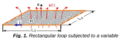
The proposed modeling approach is based on the Faraday's law applied to a closed rectangular loop as illustrated in Fig. 1. The analytical calculation of the active loss can be performed in the typical parallelepipedic subdomain supposed to be subjected by an exciting variable flow as can be seen in Fig. 2.
2.1.1 Study of a closed rectangular loop subjected to a variable flow
The figure Fig.2 below shows this loop.
ϕ (t): variable magnetic flow of exciting induction z: revolutionary axis of the loop
μ: magnetic permeability of the domain locked up by the loop L1 and L2: length and width of the loop
i: induced current
Fig. 1. Rectangular loop subjected to a variable flow ____________________________
Dr Tsialefitry ALY SAANDY is currently Professor of electric machines and electric power in the physical department of Faculty of Sciences , University of Antsiranana, Madagascar, PH-261 34 03 830 08. E-mail: [email protected]
Pr Minoson RAKOTOMALALA is Professor in the University of Antananarivo (Madagascar) and Director of the Institute for the Energy Control, PH-261 34 9672047.
E-mail: [email protected]
Dr SAÏD MZÉ is currently Professor of electric machines and distribution network of electrical power electric power in the department energy genius of Higher Teacher Training School for Technical Teaching , University of Antsiranana, Madagascar, PH-2613407 03907, E-mail: [email protected]
Avisel Fredo Toro, Research Student, Physical Department of Faculty of Sciences, PH-261 32 78 144 18,
E-mail: [email protected].
Antonio Jaomiary, Research Student, Physical Department of Faculty of Sciences, E-mail: [email protected]
By hypothesis, the loop is assumed to be placed in a domain of permeability µ and also supposed to be subjected by a variable flow. Consequently, the loop is fed by an induced e.m.f. e which induced then the loop current [12], [13], [14]. The loop e.m.f. e is a voltage source connected to the passive RL load which is constituted by a resistance in series or parallel with an inductance. The loop resistance consumes an active power which will be calculated here after. Knowing the magnetic induction and the loop surface geometrical parameters, the flux and the induced e.m.f. can be written as:
S S d B dt d e(1)
In other words, the loop can be also defined by its electrical equivalent circuit, by the time-dependent differential equations:
(2)
With an exciting flow Ф of pulse ω, equations (2) and (3) give one of the diagrams in the Fig. 2a and 2b.
(3)
With an exciting flow Ф of pulse ω, equations (2) and (3) give one of the diagrams in the Fig. 2a and 2b.
Fig.2a. Temporal electric model of a loop subjected to
a variable flow
Fig.2b. Complex electric model of a loop subjected to a
variable flow
e: instantaneous induced tension
i: intensity of the instantaneous induced current ir: component of i passing in rp
: component of i passing in E: complex induced tension.
I: intensity of the complex induced current Ir: component of I passing in rp
: component of I passing in ω: pulse of exciting flow Ф
The active power consumed by the whorl is given by the law of Joule.
for the Fig. 2a
2 si r
p (4)
for the Fig. 2b
2 r pi r
p (5)
Expressions (4) and (5) give the same active power.
2 r p 2 si ri r
p (6)
Resistances rs and rp as well as inductances sand p are
bound by the following relations.
p 2 p 2 2 p
2 p 2
s
p 2 p 2 2 p
2 p 2
s
r
r r
r
(7)
In equation (3), E and I indicate respectively the modules of the complex voltage E and current I. E and I are equal to the effective values of e and i.
2.1.2 Study of a parallelepipedic domain subjected to an exciting to a variable flow
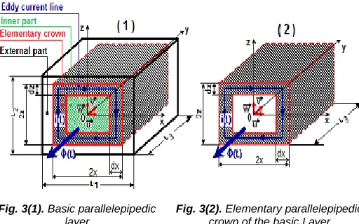
The studied domain is a parallelepiped having geometrical length L1 width L3 and thickness L2 as explained by Fig. 3(1). It
is crossed by a variable magnetic flux Ф(t) according to its length [5], [6], [7], [8], [9], [10]. An element of crown L1 length,
width 2x and thickness 2z, having elementary thicknesses dx according to x and dz according to z, divides the domain into two parts Fig. 3(1) and Fig. 3(2):
outer part, inner part.
272 Fig. 3(1). Basic parallelepipedic
layer
Fig. 3(2). Elementary parallelepipedic crown of the basic Layer
The fictitious parallelepipedic crown of the Fig. 3(2) is comparable to a closed rectangular loop, traversed by a induced current i by the exciting variable magnetic flux Ф(t). It wraps the inner part of the basic parallelepiped having magnetic permeability μ. Proportional cutting [5] is added to the model suggested by [8] to obtain the following relation.
k L L dx dz x z
1 2
(8)
The elementary resistance of the fictitious parallelepipedic crown of the Fig. 3(2) is worth:
dx x k
k 1 L 4 zdz xdx dxdz L
4 r
2
3 Fe
3
Fe
(9)
The parallel configuration is used to calculate the active power. This elementary resistance consumes the active power p such as:
p 2
p 2
r Bxz 4 r E
p (10)
The formulas (12) and (13) give:
dx x B k 1
k L 4
p 2 2 3
2 3
Fe
3
(11)
The active power of the layer is worth:
2 2 2 3 4 1 3 2
Fe
2 1 L
0 3 2 2 2 3
Fe 3
domain domain
B f k 1
k L L 16
1
dx x B k 1
k L 4 p p P
(12)
2.2 Description of the Single Phase Transformer Under Study
Fig. 4 represents the photograph of the single phase transformer. The corresponding structure including the geometrical dimensions is illustrated by Fig. 5.
Fig. 4. Photograph of the Single Phase Transformer Understudy
Fig. 5: Physical diagram of the studied transformer
a1 = 16.5 cm: external length of the core
a2 = 16.5 cm: external height of the core
a3 = 5.5 cm : external width of the core
a4= 2 cm: width of the outer wings of the core
a5 = 4 cm: width of the central wing of the core
N1 = 220: whorls turn of the primary winding
N2 = 115 : whorls turn of the secondary winding
f : mean length of the field route
The 3D structure diagram of the studied transformer shown in Fig. 5 is manly constituted by:
a core obtained by stacking of Nf layers in E and I form.
The mean length f of the field route in the core is
determined by:
4 2 1 2a 2a
a
f
(13)
two concentric coils with N1 whorls for the primary winding
and N2 for the secondary.
2.3 Determination of the Steinmetz Coefficient of the Eddy Current Loss in the Core
2.3.1 Simplifying assumptions
The following simplifying assumptions are adopted: Permanent mode at the industrial frequencies; Isotropy of the transformer core;
Constancy of the iron conductivity;
Absence of the skin effect in each layer used to form the transformer core;
Active loss due to the Eddy current loss in the transformer core;
Weakness of the hysteresis loss in front of the Eddy current loss;
Possibility of passing from series configuration to parallel configuration and vice versa;
2.3.2 Calculation of Eddy current loss in the core and Steinmetz coefficient expression
As the core counts Nf layers, the total active power which it
consumes has the expression below:
2 2 2 3 4 1 3 2 Fe f domain f
Fe f B
k 1 k L L 16 N P N P (14)
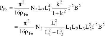
The formulas (8) and (14) give the final expression of the iron loss of a single-phase transformer below.
2 2 2 2 3 2 1 2 2 2 1 2 1 f Fe 2 2 2 2 2 4 1 3 f Fe 2 Fe B f L L L L L L L N 16 B f k 1 k L L N 16 P (15)
The definition of the specific loss of sheet for the electric machines makes possible to express the Eddy current by the formula below.
2 2 2 Fe K.V.s f B
P (16)
where
K: Eddy currents Steinmetz coefficient; B : effective value of induction in the plate ;
V : volume of the material through which passes the flow of the induction B;
s : thickness of the sheet;
The constant K in the formula (16) has the unit of electric conductivity. The identification between the formula (15) and formula (16) gives:
(17)
The constant K in the formula (17) has also the unit of electric conductivity. It is the Steinmetz coefficient for a shell form single-phase transformer. This expression is also valid for a core form transformer. For a toroidal transformer, the thickness L2 is kept but the width L1 is calculated according to the
conservation of volume for a length equalizes with the perimeter corresponding to the average radius of the torus.
L1 is worth:
in out
1 R R
L , (18)
where
Rout: external radius of the torus
Rin: inner radius of the torus
Thereafter, the width will be noted w and the thickness s. The attenuation factor of the Steinmetz coefficient becomes:
2 2 2 x 1 1 w s 1 1 A (19) where
s : thickness of the sheet;
w: width of the sheet surface crossed by the magnetic flow.
w s
x (20)
2.3.3 From the Specific Loss to the resistivity of a sheet
The manufacturers give often the specific loss of a sheet but not its resistivity. This specific loss is given in experiments. It has like unit W/kg. Its expression is:
1000 * d V P P Fe Fe Fe
S (21)
where
PS : Specific loss given by manufacturers ;
PFe : Iron loss of the transformer;
VFe : Iron volume of the transformer;
dFe : Iron density equalizes to 7.87.
By substituting (16) into formula (21), we have:
3 Fe 2 2 2 2 2 2 Fe 2 Fe 2 2 2 S 10 d B f . s w s w 16 1000 * d B f s .. K P (22)
The resistivity is drawn from formula (22) as below:
3 2 2 2 2 2 2 S 2
Fe f B 10
s w s w P 92 . 125 ρ (23)
2.4 Experimental checking of the model
The experimental setup corresponding to the performed open circuit with the shell form single-phase transformer of 1 kVA to check the model is illustrated in Fig. 6.
Fig. 6 : Wiring diagram for open circuit test
u : alternative voltage source.
ATR: auto-transformer supplied with u. TR: tested transformer
u10: primary no-load voltage.
V1: voltmeter measuring the effective value of the primary
voltage u10
i10: primary no-load current.
A: ammeter measuring the effective value of the current i10.
274 U20: secondary no-load voltage.
V2: voltmeter measuring the effective value of the secondary
voltage u20
N1: primary whorls number.
N2: secondary whorls number
From the open-circuit test, it is possible to obtain: the effective value B of induction in the core
5 3 2
20 a a fN 2
U B
(24)
the effective value H of the magnetic field in the core
f 10 1
I
N
H
(25)3
R
ESULTS ANDD
ISCUSSIONS3.1 Theoretical point of view
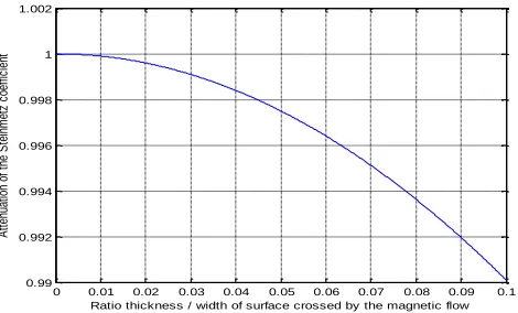
According to [13] and [14], the parameter x must be between 0 and 0.1 (0< x < 0.1). Thus, formula (19) gives the curve of the Steinmetz coefficient attenuation below.
0 0.01 0.02 0.03 0.04 0.05 0.06 0.07 0.08 0.09 0.1 0.99
0.992 0.994 0.996 0.998 1 1.002
Ratio thickness / width of surface crossed by the magnetic flow
A
tt
en
ua
tio
n
of
t
he
S
te
in
m
et
z
co
ef
fic
ie
nt
Fig. 7: Attenuation of the Steinmetz coefficient in function of ratio thickness/width of surface crossed by the flow
The Steinmetz coefficient can be extracted from (16) in function of the constant K. The model enables to express the same power as defined in formula (15). However, the attenuation coefficient varies from 1 to 0.99 as can be understood in Fig. 7. Consequently, the relative error can be neglected and allowing us to use A≈1.
3.2 Practical point of view
The results presented in this section are obtained with the transformer photographed in Fig. 3. Each element constituting the layers is suitably compared to the basic layer in Fig. 5a. It is worth noting that the transformer characteristic B(H) is not available in our laboratory. Therefore, the transformer core experimental characterization was carried out. As results, we reconstructed via vector fitting the curve plotted in Fig. 8. The red line of the curve plotted in Fig. 8 represents the considered transformer core characteristic B(H). The results of measurement using the secondary winding as sensor approach this curve. The current in the secondary voltmeter presents a low level and does not disturb enough the field.
0 10 20 30 40 50 60 70 80
0 0.2 0.4 0.6 0.8 1 1.2 1.4 1.6
Applied magnetic field H in A/m
M
a
g
n
e
ti
c
f
lu
x
d
e
n
s
it
y
B
i
n
T
Smoothed Characteristic B(H) from measurements Measurement results using no-load test
Fig. 8: Characteristics B(H) of the transformer core
This characteristic is necessary for computing the efficient value of induction and open-circuit active power of the transformer. These results are deduced from the open circuit test of which curves are depicted in Fig. 9.
0 50 100 150
0 50 100 150 200 250
No-load Primary current in mA
N
o
-l
o
a
d
P
ri
m
a
ry
a
n
d
s
e
c
o
n
d
a
ry
v
o
lt
a
g
e
s
i
n
V
Smoothed no-load primary voltage Measurement no-load primary voltage Smoothed no-load secondary voltage Measurement no-load secondary voltage
Fig. 9 : Open-circuit test characteristic of the transformer under study
In this open-circuit characteristic, the magenta and blue curves represent respectively the primary and secondary voltage calculated using the smoothed characteristic B(H). The measurements are in good agreement with the secondary smoothed voltage. This result confirms the good choice of the secondary like sensor of B. For the primary, the open-circuit measured voltage is lower than the smoothed data. There is an effect of leakage impedance of the primary winding. F. STEFENS [8], A. Mouillet, M. Akroune, M. Dami [13] and Jean-Claude BAVAY, Jean VERDUN [14] give PS = 3 W/kg to 1.5 T
for a FeSi sheet of thickness 35/100 mm intended for the construction of transformers. The formula (23) gives the
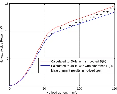
0 50 100 150 0
5 10 15
No-load current in mA
N
o
-l
o
a
d
A
c
ti
v
e
P
o
w
e
r
in
W
Calculated to 50Hz with smoothed B(H) Calculated to 48Hz with with smoothed B(H)
Measurement results in no-load test
Fig. 10: Open-circuit active power of the tested transformer
The measured values which are represented by the data plotted in the black crosses, lie between the minimal and maximal values of the theoretical calculated active power.
4
C
ONCLUSION ANDF
UTUREW
ORKA modeling method of the Steinmetz coefficient corresponding to the Eddy current losses from a single-phase transformer is proposed. The analytical calculations were carried out based on the transformer shell form. The obtained results can be employed for the calculation of the active loss in an electromagnetic domain of other forms such core form and toroidal form. In addition, the proposed modeling method can be exploited to determine the electric resistivity of an unspecified magnetic circuit as established in formula (22). Theoretical consumption was expressed according to the values of resistivity using the specific loss as suggested in [12] and [13]. More importantly, the maximal and minimal shift frequency due to the local electrical network instability was taken into account. The experimental results lie between the computed values at the two frequencies. The resistivity deduced from the specific loss by using the model is different of the resistivity given by the documents treating the FeSi alloys. However, the specific loss corresponds to coherent results with the experimental results. These results do not include the hysteresis loss. The characteristic of alloy constituting the core is not given. Collaboration with manufacturers of sheets for the electric machines to have fuller information is necessary. A good correlation between the practical and theoretical results was verified with the proposed approach. In the future, we expect to extend the proposed model to the larger fields of applications as electrical rotating machines modeling.
A
CKNOWLEDGMENTThe authors wish to thank SWERTA team for its help as well.
R
EFERENCES[1] J.Simon C. Bell and Pat S. Bodger, ―Power transformer design using core theory and finite element analysis-a comparison of techniques‖. Presented in AUPEC 2007, Perth, Western Australia, 9-12 December, 2007 ; p 2-5
[2] Claude CHEVASSU, ‗‘Machines électriques: cours et problèmes‘‘; Date: 20 juillet 2012 pp 27-33 modifié le 26/09/2013 07 :15
[3] Bernard MULTON ‗‘Modèles électriques du transformateur électromagnétique‘‘, Antenne de Bretagne de l‘École Normale Supérieure de Cachan. Revue 3EI décembre 1997 ; pp. 2-5
[4] Nicola Chiesa, ‘’Power Transformer Modeling for Inrush Current Calculation‘‘, Thesis for the degree of Philosophiae Doctor Trondheim, June 2010 modified le 20/06/2014 12:11 pp. 10-33.
[5] Jean RALISON, Tsialefitry ALY SAANDY, Avisel Fredo TORO et Jeannot VELONTSOA. «Impact du courant de Foucault sur la détermination des éléments du schéma équivalent d‘un transformateur monophasé». Afrique Science, Vol.11, N°4 (2015), 1 juillet 2015, http://www.afriquescience.info/document.php?id=4878. ISSN 1813-548X.
[6] David W. Johnson, ‗‘The Transformer Equivalent Circuit From Experiment‘‘, Grand Valley State University, Padnos School Of Engineering , April 17, 2000 modified le 20/06/2014 12 :23 pp. 2-4
[7] Kharagpur University, ―Cores and Core Losses‖ Version 2 EE IIT, Kharagpur. Module 6, pp. 4-16
[8] – F.STEFENS: "PHYSIQUE GENERAL. Electrostatique. Electromagnétisme": EDIDEPS.Kinshasa.1985, pp. II73-II74
[9] Bernaud J. ‗‘Transformateur monophasé Chapitre B 2.1‘‘ modifié le 09/03/2013 ; 19 :23 http://lyc-renaudeau-49.ac-nantes.fr/physap/IMG/pdf/E_2_tra_co_version_a_trou.pdf pp 2-9
[10]Ruchi Singuor, Priyanka Solanki, Neeti Pathak, D. Suresh Babu,‘‘Simulation of Single Phase Transformer with Different Supplies‘‘, International Journal of Scientific and Research Publications, Volume 2, Issue 4, April 2012 ISSN 2250-3153
[11]Samet BIRICIK, Özgür Cemal ÖZERDEM, ‗‘A Method For Power Losses Evaluation In Single Phase Transformers Under Linear And Nonlinear Load Conditions‘‘, Near East University, Dep. of Electrical & Electronic Engineering, N. Cyprus, Przegląd Elektrotechniczny (Electrical Review), Issn 0033-2097, R. 87 Nr 12a/2011 Pp. 74-77
[12]Gabriel Cormier, ‗‘Circuits Magnétiques et Inductance‘‘, Chapitre 7, GEN1153, p 6
[13]A. Mouillet, M. Akroune, M. Dami, « Caractérisation des tôles Fer-Silicium en régime dynamique, pulsant ». Journal de Physique IV, 1992, 02 (C3), pp.C3-53-C3-58. <10.1051/jp4:1992307>.,<jpa-00251512>