A System Level Approach to Optimal Controller Design for Large-Scale Distributed Systems

(1)

for Large-Scale Distributed Systems

Thesis by

Yuh-Shyang Wang

In Partial Fulfillment of the Requirements for the degree of

Doctor of Philosophy

CALIFORNIA INSTITUTE OF TECHNOLOGY Pasadena, California

2017

(2)

(3)

ACKNOWLEDGEMENTS

First of all, I would like to express my deepest thank to my advisor, Professor John Doyle, for his enthusiastic guidance and support during my graduate school years. John is an incredibly inspiring scholar. His unique insight into the fundamental problems across a broad range of different fields has broadened my view of scientific research. He gave me many brilliant ideas, encouraged me to pursue my own research directions, and gave me great freedom to work on the most exciting projects that I could ever find. I am so grateful to be his student in my time at Caltech.

I also want to express my thank to my thesis committee: Professors Richard Murray, Adam Wierman, and Soon-Jo Chung. Their comments and suggestions have greatly helped improve the quality of this dissertation. Richard has supported me at each stage of my graduate study, and gave me valuable advices for my career plan. I am also thankful to Professors Steven Low, Lijun Chen, and Venkat Chandrasekaran for introducing me to the field of power network and optimization.

Special thanks to Nikolai Matni for his mentorship in my whole graduate student years. Nikolai works as my “technical advisor" at Caltech. He helped me clarify technical details of my results and guided me step by step in scientific writing and presentation. This thesis would not have been completed without his help. I am also thankful for the guidance from Seungil You in my early time at Caltech, and Changhong Zhao for the questions in power systems.

Thanks to my friends in the CDS department: Yoke Peng, Yorie, Ioannis, Ania, Thomas, Niangjun, Noah, Dimitar, John, and all my friends in the Annenberg community. Thanks to the help from the staff members in the CMS department, especially Maria and Nikki. I would also like to express my thank to all my friends in Caltech, especially from the Association of Caltech Taiwanese and Caltech Badminton Club.

(4)

ABSTRACT

Modern cyber-physical systems, such as the smart grid, software-defined networks, and automated highway systems, are large-scale, physically distributed, and inter-connected. The scale of these systems poses fundamental challenges for controller design: the traditional optimal control methods are globally centralized, which re-quire solving a large-scale optimization problem with the knowledge of the global plant model, and collecting global measurement instantaneously during implementa-tion. The ultimate goal of distributed control design is to provide a local, distributed, scalable, and coordinated control scheme to achieve centralized control objectives with nearly global transient optimality.

This dissertation provides a novel theoretical and computational contribution to the area of constrained linear optimal control, with a particular emphasis on addressing the scalability of controller design and implementation for large-scale distributed systems. Our approach provides a fundamental rethinking of controller design: we extend a control design problem to a system level design problem, where we directly optimize the desired closed loop behavior of the feedback system. We show that many traditional topics in the optimal control literature, including the param-eterization of stabilizing controller and the synthesis of centralized and distributed controller, can all be cast as a special case of a system level design problem. The sys-tem level approach therefore unifies many existing results in the field of distributed optimal control, and solves many previously open problems.

(5)

(6)

PUBLISHED CONTENT AND CONTRIBUTIONS

[1] Yuh-Shyang Wang. “Localized LQR with Adaptive Constraint and Perfor-mance Guarantee”. In:to appear in 2016 55th IEEE Conference on Decision

and Control (CDC). 2016.

Y.-S. Wang proposed the original idea of the paper. The content of this paper is described in Section 5.5 in this dissertation.

[2] Yuh-Shyang Wang and Nikolai Matni. “Localized Distributed Optimal Con-trol with Output Feedback and Communication Delays”. In: IEEE 52nd

An-nual Allerton Conference on Communication, Control, and Computing. 2014. doi:10.1109/ALLERTON.2014.7028511.

Y.-S. Wang proposed the original idea of the paper. This paper is the prelim-inary version of [3].

[3] Yuh-Shyang Wang and Nikolai Matni. “Localized LQG Optimal Control for Large-Scale Systems”. In:2016 IEEE American Control Conference (ACC). 2016. doi:10.1109/ACC.2016.7525205.

Y.-S. Wang proposed the original idea of the paper. The content of this paper is described in Chapter 6 in this dissertation.

[4] Yuh-Shyang Wang, Nikolai Matni, and John C. Doyle. “A System Level Approach to Controller Synthesis”. In: submitted to IEEE Transactions on

Automatic Control(2016).

Y.-S. Wang proposed the original idea of the paper. The content of this paper is covered in Chapter 1 to Chapter 4 in this dissertation.

[5] Yuh-Shyang Wang, Nikolai Matni, and John C. Doyle. “Localized LQR Con-trol with Actuator Regularization”. In:2016 IEEE American Control

Confer-ence (ACC). 2016. doi:10.1109/ACC.2016.7526485.

[6] Yuh-Shyang Wang, Nikolai Matni, and John C. Doyle. “Localized LQR Op-timal Control”. In: 2014 53rd IEEE Conference on Decision and Control

(CDC)_{. 2014. doi:}10.1109/CDC.2014.7039638_.

Y.-S. Wang proposed the original idea of the paper. The content of this paper is described in Chapter 5 in this dissertation.

[7] Yuh-Shyang Wang, Nikolai Matni, and John C. Doyle. “Localized System Level Synthesis for Large-Scale Systems”. In:submitted to IEEE Transactions

on Automatic Control(2016).

Y.-S. Wang proposed the original idea of the paper. The content of this paper is covered in Chapter 5 to Chapter 7 in this dissertation.

(7)

Control Conference (ACC). 2017.

Y.-S. Wang proposed the original idea of the paper. This paper is the simplified version of [4].

[9] Yuh-Shyang Wang, Seungil You, and Nikolai Matni. “Localized Distributed Kalman Filters for Large-Scale Systems”. In: 5th IFAC Workshop on

Dis-tributed Estimation and Control in Networked Systems. 2015. doi:10.1016/

j.ifacol.2015.10.306_.

[10] Yuh-Shyang Wang et al. “Localized Distributed State Feedback Control with Communication Delays”. In:2014 IEEE American Control Conference

(ACC). June 2014. doi:10.1109/ACC.2014.6859440.

(8)

LIST OF ILLUSTRATIONS

Number Page

1.1 Optimal Feedback Control Problem . . . 4

1.2 Relations between the traditional constrained optimal control frame-work and the system level synthesis frameframe-work . . . 6

1.3 Examples of CLS-SLS problems . . . 7

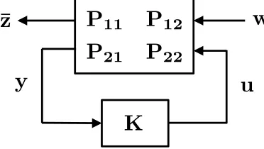
2.1 Interconnection of the plantPand controllerK. . . 11

2.2 An illustration of the system response in the block diagram . . . 16

2.3 The proposed output feedback controller structure, with R˜+ = zR˜ = z(I −zR)_,M˜ = zM_{, and}N˜ =−zN_. _{. . . .} ₁₇

2.4 Internal stability analysis diagram . . . 20

3.1 The proposed state feedback controller structure, with R˜ = I − zR andM˜ = zM. . . 25

3.2 The proposed output feedback controller structure, with R˜+ = zR˜ = z(I −zR)_,M˜ = zM, andN˜ =−zN. . . 30

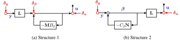
3.3 Alternative controller structures for stable systems. . . 34

(a) Structure 1 . . . 34

(b) Structure 2 . . . 34

3.4 The proposed output feedback controller structure forD22 , 0. . . 36

4.1 Space time diagram for a single disturbance striking the chain de-scribed in Example 3. . . 53

5.1 An Example of Interconnected System . . . 59

5.2 Illustration of the 2-incoming and 2-outgoing sets of subsystem 5. . . 65

5.3 The localized region forw1. . . 70

5.4 Information delay and physical delay . . . 77

5.5 Localized region for the initial condition x[1]= e1in a large network 84 5.6 Lower bound problem for Figure 5.5 . . . 87

5.7 Upper bound problem for Figure 5.5 . . . 88

5.8 Performance vs. FIR horizonT and localized region d. The cost is normalized with respect to the optimal centralizedH2cost. . . 99

(11)

5.10 Interconnected topology for the simulation example . . . 100

5.11 Computation time for the centralized, distributed, and localized LQR 102 6.1 An Example of Interconnected System . . . 105

6.2 Simulation example interaction graph. . . 114

(a) Interconnected topology . . . 114

(b) Interaction between neighboring subsystems . . . 114

6.3 The vertical axis is the normalizedH2norm of the closed loop when the LLQG controller is applied. The LLQG controller is subject to the constraintC ∩ L ∩ FT. The horizontal axis is the horizonT of the FIR constraintFT, which is also the settling time of the impulse response. We plot the normalized H2 norm for the centralized unconstrained optimal controller (proper and strictly proper) in the same figure. . . . 116

6.4 Computation time for the centralize, distributed, and localized LQG controller. The horizontal axis denotes the number of states of the system, and the vertical axis is the computation time in seconds. . . . 118

7.1 The upward-pointing triangles represent the subsystems in which the PMU is removed. The downward-pointing triangles represent the subsystems in which the controllable load (actuator) is removed. . . . 139

(12)

LIST OF TABLES

Number Page

3.1 Closed Loop Maps from Perturbations to Internal Variables . . . 32 5.1 Closed Loop Maps With Non-localizability . . . 82 5.2 Comparison Between Centralized, Distributed and Localized LQR

on a 51200-State Randomized Example . . . 103 6.1 Comparison Between Centralized, Distributed, and Localized LQG

(13)

C h a p t e r 1

INTRODUCTION

Large-scale networked systems have emerged in extremely diverse application ar-eas recently, with examples including the smart grid, automated highway systems, software-defined networks, Internet of Things, and biological networks in science and medicine. These systems often have limited, sparse, uncertain, and distributed communication and computing in addition to sensing and actuation. Fortunately, the corresponding plants and performance requirements are also sparse and struc-tured, and this must be exploited to make constrained controller design feasible, tractable, and scalable. In this dissertation, we introduce a new “system level" (SL) approach involving three complementary SL elements. System Level Parameteri-zations (SLPs) generalize state space and Youla parameteriParameteri-zations of all stabilizing controllers and the responses they achieve, and combine with System Level Con-straints (SLCs) to parameterize the largest known class of constrained stabilizing controllers that admit a convex characterization, generalizing quadratic invariance (QI). The resulting System Level Synthesis (SLS) problems that arise define the broadest known class of constrained optimal control problems that can be solved using convex programming. Furthermore, we identify a class of SLS problem, which is called the convex localized separable SLS (CLS-SLS) problems, that can be solved withO(1)computational complexity. The class of CLS-SLS problems, which include the localized H2 optimal control with sensor actuator

regulariza-tion and the localized mixed H2/L1optimal control problem as special cases, are

therefore scalable to systems with arbitrary large-scale. In the following, we review the literature in the field of constrained optimal control, present the key ideas and main contributions of our method, and outline the organization of the rest of this dissertation.

1.1 Motivation and Challenges

(14)

ad-vantage of this approach is that an affine expression of the Youla parameter describes all achievable responses of the closed loop system, allowing for system behavior to be directly optimized. Together with state-space methods, this contribution played a major role in shifting controller synthesis from an ad hoc, loop-at-a-time tuning process to a principled one with well defined notions of optimality. Indeed, this approach proved very powerful, and paved the way for the foundational results of robust and optimal control that would follow [13].

This dissertation presents an approach that is inspired by the system level thinking pioneered by Youla: rather than directly designing only the feedback loop between sensors and actuators, we propose directly designing theentire closed loop response

of the system_{, as captured by the maps from process and measurement disturbances}

to control actions and states — as such, we call the proposed method a system level approach to controller synthesis. A distinction between our approach and Youla’s is that we explicitly model the internal delay structure of the feedback system, whereas Youla (and contemporary state-space methods) hid the internal structure of the controller, and focused instead on its input-output behavior. This focus on controller input-output behavior was natural for the problems of that era (often motivated by aerospace and process control applications), where systems had a single logically centralized controller with global access to sensor measurements and global control over actuators.

In contrast, modern cyber-physical systems (CPS) are large-scale, physically dis-tributed, and interconnected. Rather than a logically centralized controller, these systems are composed of several sub-controllers, each equipped with their own sen-sors and actuators — these sub-controllers then exchange locally available informa-tion (such as sensor measurements or applied control acinforma-tions) via a communicainforma-tion network. It follows that the information exchanged between sub-controllers is con-strained by the delay, bandwidth, and reliability properties of this communication network, ultimately manifesting as information asymmetry among sub-controllers of the system. It is this information asymmetry, as imposed by the underlying communication network, that lies at the heart of what makes distributed optimal controller synthesis challenging [2, 3, 23, 37, 46, 53].

(15)

Further, there was reason to suspect that introducing such information asymmetry into the optimal control problem lead to intractable synthesis tasks [4, 61, 76]. Despite these apparent technical and conceptual challenges, a body of work [2, 3, 14, 37, 46, 49, 53] that began in the early 2000s, and culminated with the introduction of quadratic invariance (QI) in the seminal paper [53], showed that for a large class of practically relevant systems, such internal structure could be incorporated into the Youla parameterization and still preserve the convexity of the optimal controller synthesis task. Informally, a system is quadratically invariant if sub-controllers are able to exchange information with each other faster than their control actions propagate through the CPS [52]. Even more remarkable is that this condition is tight, in the sense that QI is a necessary [33] and sufficient [53] condition for subspace constraints (defined by, for example, communication delays) on the controller to be enforceable via convex constraints on the Youla parameter.

The identification of QI as a useful condition for determining the tractability of a distributed optimal control problem led to an explosion of synthesis results in this area [27, 29, 30, 32, 34, 42, 55, 57, 59]. These results showed that the robust and optimal control methods that proved so powerful for centralized systems could be ported to distributed settings. However, they also made clear that the synthesis and implementation of QI distributed optimal controllers did not scale gracefully with the size of the underlying CPS. In particular, a QI distributed optimal controller is at least as expensive to compute as its centralized counterpart (c.f., the solutions presented in [27, 29, 30, 32, 34, 42, 55, 57, 59]), and can be more difficult to implement (c.f., the message passing implementation suggested in [29]).

We show in Chapter 2 that the QI framework, which adapts the Youla parameteri-zation to a distributed setting, fails to capture certain constraints that are needed for optimal controller synthesis to scale to arbitrarily large systems. In particular, when the underlying physical system is strongly connected,1 the QI framework does not allow for localized controllers, in which local sub-controllers only access a subset of system-wide measurements (c.f., Section 4.2.8), to be synthesized using convex programming; perhaps counter-intuitively, this statement holds true even when sub-controllers can exchange information with no delay (c.f., Example 1). Although this may seem surprising, note that implicit to the Youla parameterization is that sub-controllers can only exchange locally collected measurements with each other,

1

(16)

and not, for instance, locally applied control actions. This restriction has no conse-quences in centralized applications, but can complicate controller implementation and synthesis in a distributed setting.

The lack of scalability of the distributed optimal control framework has not gone unnoticed by the community, and techniques based on regularization [17, 35], convex approximation [16, 19, 65], spatial truncation [45], and structural realization [62–64] have been used in hopes of finding a sparse (structured) feedback controller that is scalable to implement. These methods have been successful in extending the size of systems for which a distributed controller can be implemented, but there is still a limit to their scalability as they often rely on an underlying centralized synthesis procedure. Further, it is not clear if these methods can be extended to compute a dynamic controller that incorporates information sharing constraints. To overcome the above-mentioned limitation, we propose the system level approach to controller synthesis [69, 72, 73], which is composed of three main elements: SLPs, SLCs, and SLS problems. We informally introduce the ideas of the system level approach as below.

1.2 Key Ideas

K

P

x

[

t

+ 1] =

Ax

[

t

] +

B

2

u

[

t

] +

x

[

t

]

y

[

t

] =

C

2

x

[

t

] +

y

[

t

]

⇠

[

t

+ 1] =

A

k

⇠

[

t

] +

B

k

y

[

t

]

u

[

t

] =

C

k

⇠

[

t

] +

D

k

y

[

t

]

y

u



x

u



x y

Figure 1.1: Optimal Feedback Control Problem

(17)

the external disturbanceδx andδy to regulated output xandu in the closed loop. The traditional way to formulate a constrained optimal control problem is typically given by

minimize

K ||Φ||

subject to Kinternally stabilizesP

K∈ C, _(1.1)

where C is a structured constraint imposed on the controller. The idea of (1.1) is to find a controllerKto optimize the closed loop system responseΦ, subject to the constraints that the interconnected feedback loop shown in Figure 1.1 is internally stable and the controller satisfies the structured constraintC. The limitation of the formulation (1.1) is that the structured constraint C usually makes the constrained optimal control problem non-convex, i.e., the QI framework only characterizes a limited class of convex problems in constrained optimal control.

The system level design philosophy approaches the constrained optimal control problem from a different point of view. Instead of designing a controller K to optimize the system responseΦ, we directly choose our desired system responseΦ from the set of all stable and achievable system response. After the desired system response Φ is chosen, we then reconstruct a controller K to achieve the desired system response. This design philosophy leads to a system level synthesis (SLS) problem given by

minimize

Φ g(Φ) (1.2a)

subject to Φstable and achievable (1.2b)

Φ∈ S, _(1.2c)

where (1.2a) is called the system level objective (SLO), (1.2b) the system level parameterization (SLP), and (1.2c) the system level constraint (SLC). The goal of this dissertation is to show that the SLS framework (1.2) offers significant benefits over the traditional frameowork (1.1) in terms of the generality, simplicity, and scalability. Our specific contributions are outlined below.

1.3 Theoretical Contributions

(18)

design problem to a system level co-design problem. For instance, we can incorpo-rate the regularizers for sensor actuator placement into the SLO in (1.2a), and use the SLS problem to co-design the controller and its sensing and actuating architecture. The set of all SLS problems is a superset of the set of all constrained optimal control problems. We show this relation using the Venn diagram in Figure 1.2.

1

NP-hard

Unknown

Constrained Optimal Control

System Level Synthesis Convex SLS

QI

LLQR

Figure 1.2: Relations between the traditional constrained optimal control framework and the system level synthesis framework

Then, we show that the SLS framework characterizes the broadest known class of constrained optimal control problems that can be solved using convex programming. This is one of the main theoretical contribution of the SLS framework. In particular, we show that the set of constrained stabilizing controllers that can be efficiently parameterized using SLPs (1.2b) and SLCs (1.2c) is a strict superset of those that can be parameterized using quadratic invariance with (1.1), and hence we provide a generalization of the QI framework, characterizing the broadest known class of constrained controllers that admit a convex parameterization. The relation between convex SLS and QI are shown in Figure 1.2.

(19)

In contrast, the theoretical computation time for the traditional LQR using the same computer is 200 days, and the distributed LQR is simply intractable. We also use an adaptive constraint update algorithm to design a LLQR controller with at least 99% optimality guarantee on the 51200-state example in 38 minutes. Table 5.2 in Chapter 5 shows the superior scalability of LLQR (a special case of a CLS-SLS problem) over the centralized and distributed approach. As shown in Figure 1.3, examples of CLS-SLS problems include localized linear quadratic Gaussian (LLQG) (the output feedback version of LLQR), localized mixed H2/L1 optimal control, and

LLQG with sensor actuator regularization using the regularization for design (RFD) framework [40, 41].

2

NP-hard

Unknown

Constrained Optimal Control

System Level Synthesis Convex SLS

CLS-SLS LLQG

H2/L1

LLQG +RFD

Figure 1.3: Examples of CLS-SLS problems

(20)

a structured controller that is scalable to implement for large-scale systems, which cannot be done using the traditional optimal control framework (1.1).

1.4 Organization of the Dissertation

The rest of this dissertation is structured as follows. In Chapter 2, we define the system model considered in the thesis, and review relevant results from the distributed optimal control and QI literature. We then provide a motivating example as to why moving beyond QI systems may be desirable, before presenting a survey of our main results. In Chapter 3 we define and analyze SLPs (1.2b) for state and output feedback problems, and provide a characterization of stable and achievable system responses. We show that SLPs also give a characterization of all internally stabilizing controllers, and propose a structural realization of the controller to achieve the desired system response. In Chapter 4, we define and analyze the SLS problem (1.2), which incorporates SLPs and SLCs into an optimization problem. We provide a catalog of SLCs that can be imposed on the system responses parameterized by the SLPs described in the previous chapter — in particular, we show that by appropriately selecting these SLCs, we can provide convex characterizations of all stabilizing controllers satisfying QI subspace constraints, convex constraints on the Youla parameter, finite impulse response (FIR) constraints, sparsity constraints, spatiotemporal constraints [67, 68, 71, 75], controller internal robustness constraints, multi-objective performance constraints, controller architecture constraints [40, 41, 70], and any combination thereof. In addition, we show that the constrained optimal control problem (1.1) is a special case of SLS (1.2).

(21)

works in Chapter 8.

1.5 Mathematical Notations

We use lower and upper case Latin letters such as x and A to denote vectors and matrices, respectively, and lower and upper case boldface Latin letters such asxand G_{to denote signals and transfer matrices, respectively. We use calligraphic letters} such asSto denote sets.

In the interest of clarity, we work with discrete time linear time invariant systems, but unless stated otherwise, all results extend naturally to the continuous time setting. We use standard definitions of the Hardy spaces H2 andH∞, and denote

their restriction to the set of real-rational proper transfer matrices by RH2 and

(22)

C h a p t e r 2

PROBLEM STATEMENT AND MAIN RESULTS

We begin by introducing the system model and some preliminaries on optimal control and Youla parameterization. We then introduce the distributed optimal control framework and discuss its limitations. This chapter ends with the summary of the main result of this dissertation.

2.1 System Model

We consider discrete time linear time invariant (LTI) systems of the form

x[t+1]= Ax[t]+B1w[t]+B2u[t] (2.1a)

¯

z[t]=C₁x[t]+D₁₁w[t]+D₁₂u[t] (2.1b) y[t]=C₂x[t]+D₂₁w[t]+D₂₂u[t], _(2.1c) wherex,u,w,y, and ¯zare the state vector, control action, external disturbance, mea-surement, and regulated output, respectively. The frequency domain representation of (2.1) is given by

zx = Ax+B₁w+B₂u

¯z = C₁x+D₁₁w+D₁₂u

y = C₂x+D₂₁w+D₂₂u, (2.2) wherezis the variable of z-transform. Equation (2.1) can be written in state space form as

P=

      

A B₁ B₂ C₁ D₁₁ D₁₂ C₂ D₂₁ D₂₂

      

= "

P₁₁ P₁₂ P₂₁ P₂₂

#

, (2.3)

wherePi j =Ci(zI− A)−1Bj+Di j. We refer toPas the open loop plant model. Remark 1. We will occasionally discuss continuous time system in this dissertation. A continuous time LTI system is given in the form

Û

x(t) = Ax(t)+B₁w(t)+ B₂u(t)

¯

z(t) = C₁x(t)+D₁₁w(t)+D₁₂u(t)

(23)

The frequency domain representation of the continuous time system is given by

(2.2) by changing z to s (the variable for Laplace transform). The state space

representation is given by(2.3), withPi j =Ci(sI −A)−1Bj +Di j.

P

11

P

12

P

21

P

22

K

y

_u

w

¯

z

Figure 2.1: Interconnection of the plantPand controllerK.

Consider a dynamic output feedback control law u = Ky. The controller K is assumed to have the state space realization

ξ[t+1]= Akξ[t]+Bky[t] (2.5a) u[t]=Ckξ[t]+Dky[t], (2.5b) whereξ is the internal state of the controller. We haveK=Ck(zI− Ak)−1Bk +Dk. A schematic diagram of the interconnection of the plant Pand the controller Kis shown in Figure 2.1.

The following assumptions are made throughout the dissertation.

Assumption 1. The interconnection in Figure 2.1 is well-posed — the matrix(I − D₂₂Dk)is invertible.

Assumption 2. Both the plant and the controller realizations are stabilizable and detectable; i.e., (A,B₂)and (Ak,Bk)are stabilizable, and (A,C₂)and(Ak,Ck) are detectable.

The internal stability of the interconnection in Figure 2.1 is defined as follows [81]. Definition 1. The interconnection in Figure 2.1 is said to be internally stable if the origin(x, ξ)=(₀,₀)is asymptotically stable, i.e.,x[t], ξ[t] →₀fort → ∞from all initial states.

(24)

useful lemmas to determine the internal stability of the interconnection in Figure 2.1 in Appendix 2.A in the end of this chapter.

The aim of the optimal control problem is to find a controllerKto stabilize the plant P and minimize a suitably chosen norm1 of the closed loop transfer matrix from external disturbancewto regulated output¯z. From the relations¯z=P11w+P12u,y =P₂₁w+P₂₂u_{, and}u=K y_{, we can express} ¯z_{as a function of}w_as

¯z= (P₁₁+P₁₂K(I−P₂₂K)−1_P 21)w.

The optimal control problem can then be formulated as minimize

K ||P11+P12K(I−P22K)

−₁ P₂₁||

subject to Kinternally stabilizesP. (2.6) We refer to (2.6) the unconstrained (centralized) optimal control problem.

2.2 Youla Parameterization

Youla parameterization is a common technique to characterize the set of all internally stabilizing controller for a given plant, i.e., the constraint set in (2.6). The Youla parameterization technique is based on a doubly co-prime factorization of the plant, which is defined as follows.

Definition 2. A collection of stable transfer matrices, Ur, Vr, Xr, Yr, Ul, Vl, Xl,

Yl ∈ RH∞defines a doubly co-prime factorization ofP₂₂ifP₂₂ = VrU−r1 =U−l1Vl

and

"

Xl −Yl

−Vl Ul

# "

Ur Yr

Vr Xr

# = I.

Such doubly co-prime factorizations can always be computed if P22 is stabilizable

and detectable [81].

LetQbe the Youla parameter. From [81], the centralized optimal control problem (2.6) can be reformulated in terms of the Youla parameter as

minimize

Q

||T₁₁+T₁₂QT₂₁||

subject to Q ∈ RH∞ (2.7)

withT11 =P11+P12YrUlP21,T12 = −P12Ur, andT21= UlP21. In (2.7), we search

over all stable proper real-rational transfer matrix Qto minimize the norm of the 1_{Typical choices for the norm include}_H

(25)

closed loop map. Once the optimal Youla parameterQis found, we reconstruct the controllerKby the formula

K= (Yr−UrQ)(Xr −VrQ)−1.

The set{(Yr−UrQ)(Xr−VrQ)−1|Q ∈ RH∞}is the parameterization of all internally stabilizing controller.

With a change of variable from controller K to Youla parameter Q, we note that (2.7) is in the form of a convex optimization problem, which can then be solved using efficient convex programming algorithms.

2.3 Distributed Optimal Control and Quadratic Invariance

Distributed optimal control problems arise when there are information asymmetry among sub-controllers in the network. In this section, we follow the paradigm adopted in [27, 30, 32, 34, 42, 53, 55, 57, 59], and focus on information asymmetry introduced by delays in the communication network — this is a reasonable modeling assumption when one has dedicated physical communication channels (e.g., fiber optic channels), but may not be valid under wireless settings. In the references cited above, locally acquired measurements are exchanged between controllers sub-ject to delays imposed by the communication network,2which manifest as subspace constraints on the controller itself.

The distributed optimal control problem is then formulated as a constrained optimal control problem in the following form [31, 33, 53, 54]:

minimize

K kP11+P12K(I −P22K)

−₁

P₂₁k _(2.8a)

subject to Kinternally stabilizesP (2.8b)

K∈ C, _(2.8c)

for Ca subspace. This subspace can enforce, for instance, the information sharing constraints imposed on the controllerKby the underlying communication network, as described above.

(26)

authors in [54] show that (2.8) can be equivalently formulated as minimize

Q ||T11+T12QT21

|| _(2.9a)

subject to Q ∈ RH∞ (2.9b)

M(Q) ∈ C_Q, _(2.9c)

whereMis an invertible affine map defined in terms of an arbitrary doubly co-prime factorization of the plant3, andCQis given by the setCQ = {K(I−P₂₂K)−1|K∈ C}. Note that the convexity of (2.9) (and/or (2.8)) depends solely on the convexity of the setCQ.

A synthesis of the main results of the distributed optimal control literature [27, 30– 34, 42, 53–55, 57, 59] can be expressed as follows: if the subspaceCis quadratically invariant (QI)4 with respect to P22 [53], then we have CQ = C, and therefore the

constraint (2.9c) can be replaced by the subspace constraintM(Q) ∈ C. In this case, problem (2.9) is a convex optimization problem. Further, the QI condition can be viewed as tight, in the sense that quadratic invariance is also anecessarycondition [31, 33] for a subspace constraintCon the controllerKto be enforced on the Youla parameterQin a convex manner.

2.4 Beyond Quadratic Invariance

We now present a simple example showing how the above framework, built around the Youla parameterization, fails to capture an “obvious” structured controller. We return to this example at the end of this chapter to show that our system level approach naturally recovers said obvious controller.

Example 1. Consider the optimal control problem:

minimize

u limT→∞

1

T

ÍT

t=₀Ekx[t]k₂2

subject to x[t+1]= Ax[t]+u[t]+w[t],

(2.10)

with zero mean unit covariance additive white Gaussian noise (AWGN) vectorw[t], i.e., w[t]i∼ N(.i.d ₀,I). We assume full state-feedback, i.e., the control action at time

t can be expressed asu[t] = f(x[_{0 :} t])for some function f. An optimal control policy u? for this linear quadratic regulator (LQR) problem is easily seen to be given byu?[t]=−Ax[t].

3_{We have}_M₍_Q₎=_K₍_I₋_P 22K)

−₁ ₌₍_Y

r−UrQ)Ul. By definition, we haveP22 =VrU−r1 = U−1

l Vl. This implies that the transfer matricesUr andUl are both invertible. Therefore,Mis an

invertible affine map of the Youla parameterQ.

4_{The subspace}_C_{is quadratically invariant with respect to}_P

(27)

Further suppose that the state matrix Ais sparse and let its support define the adja-cency matrix of a graphGfor which we identify theith node with the corresponding state/control pair (xi,ui). In this case, we have that the optimal control policyu?

can be implemented in alocalizedmanner. In particular, in order to implement the

state feedback policy for theith actuatorui, only those states xj for which Ai j , 0

need to be collected — thus only those states corresponding to immediate neighbors

of nodei in the graphG, i.e., onlylocalstates, need to be collected to compute the

corresponding control action, leading to a localized implementation. As we discuss

in more detail in Section 4.2.8 and in Chapter 5 - 7, the idea of locality is essential

to allowing controller synthesis and implementation to scale to arbitrarily large

systems, and hence such a structured controller is desirable.

Now suppose that we naively attempt to solve optimal control problem (2.10) by

converting it to its equivalent H₂ optimal control problem and constraining the controller K to have the same support as A, i.e., K = Í∞

t=₀ z1tK[t], supp(K[t]) ⊂ supp(A). If the graph G is strongly connected, then the conditions in [52] imply

that the corresponding distributed optimal control problem is not quadratically

invariant. The results of [33] further allow us to conclude that computing such a

structured controller cannot be done using convex programming when using the

Youla parameterization described in the previous section.

In addition, we note that the QI framework is developed under the assumption thatC in (2.8c) is asubspaceconstraint. WhenCis not a subspace constraint, no general method exists to determine the convexity of the constrained optimal control problem (2.8). Further, we note that the optimization problem (2.9) is convex as long as the set CQin (2.9c) is a convex set — in particular, the setCQdoes not need to satisfy the QI condition, nor doesCQneed to be a subspace. In other words, there are some convex constrained optimal control problems that cannot be identified using the theory of QI. The motivation of this thesis is to generalize the QI framework to characterize a broader class of convex constrained optimal control problems, and show that some of these problems are extremely favorable for large-scale applications.

2.5 Summary of Main Results

(28)

equation (2.8).

For a LTI system with dynamics given by (2.1), we define asystem response{R,M, N,L} to be the closed loop maps satisfying

"

x u

# =

"

R N

M L

# "

δx

δy #

, (2.11)

where δx = B1w is the disturbance on the state vector, and δy = D21w is the

disturbance on the measurement. We illustrate the system response using the block diagram shown in Figure 2.2.

Figure 2.2: An illustration of the system response in the block diagram We say that a system response {R,M,N,L} isstable and achievable with respect to a plantPif there exists an internally stabilizing controllerKsuch that the inter-connection illustrated in Figure 2.1 leads to closed loop behavior consistent with equation (2.11).

(29)

if it lies in the affine subspace described by:

h

zI− A −B₂

i "

R N

M L

#

= hI 0

i

(2.12)

"

R N

M L

# "

zI− A −C₂

# =

"

I

0

#

(2.13) R,M,N∈ 1

zRH∞, L ∈ RH∞. (2.14)

As the above characterizes all stable and achievable system responses, we call it a system level parameterization (SLP).

In addition, for such a stable achievable system response {R,M,N,L}, a controller that leads to these closed loop maps is given by K = L −MR−1N, and can be implemented as:

zβ = z(I−zR)β−zNy

u = zMβ+Ly, (2.15)

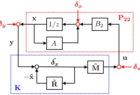
forβthe internal state of the stabilizing controller.5 A block diagram of the controller structure is shown in Figure 2.3.

B2

1/z

A

1/z C2

y

x

u x

u y

˜ M

L ˜

N

˜ R+

Figure 2.3: The proposed output feedback controller structure, with R˜+ = zR˜ = z(I−zR)_,M˜ = zM_{, and}N˜ =−zN_.

Notice that any sparsity structure imposed on the system response {R,M,N,L} translates directly to the sparsity structure of the controller implementation, and hence information sharing constraints on the measured outputyand controller stateβ can be imposed via subspace constraints on the system response{R,M,N,L}. As the

5

(30)

controller is implemented directly using these transfer matrices, we are furthermore no longer limited to subspace constraints, and can in fact impose arbitrary system level constraints (SLCs) on the closed loop response of the system, and by extension the controller implementation. In Section 4.2, we provide a catalog of useful SLCs. We also show in Section 4.2.1 and 4.2.2 that by combining appropriate SLCs with the SLP (2.12) - (2.14), we recover all structured controllers that can be parameterized using the Youla parameter and quadratic invariance.

Let S denote such a SLC, and assume that it admits a convex representation. Furthermore, let g(·) be a convex functional. This gives a convex system level synthesis (SLS) problem

minimize

{R,M,N,L} g(R,M,N,L) (2.16a) subject to equations (2.12)−(2.14) (2.16b)

"

R N

M L

#

∈ S. _(2.16c)

We show in Chapter 4 that the SLS problem (2.16) characterize the broadest known class of convex problems in optimal control — in particular, the distributed optimal control problem (2.8) is a special case of a SLS problem. Beside (2.8), we show that the mixed objective optimal control problem and the sensor actuator regularized optimal control problem can all be cast as a SLS problem.

In Chapters 5 - 7, we focus on a special class of SLS problems, which we call the convex localized separable SLS (CLS-SLS) problems. By imposing suitable localized SLC in (2.16c), we show that the CLS-SLS problems can be solved in an extremely scalable manner, i.e., withO(1)parallel computational and implementa-tion complexity relative to the size of the overall system. This allows us to synthesize and implement localized optimal controller for systems with arbitrary large-scale, which is extremely favorable for large-scale applications.

Example 2(Example 1 cont’d). We now return to the motivating example introduced

above to provide a preview of the usefulness of the system level approach to controller synthesis. In the case of a full control (B₂ = I) state-feedback (C₂ = I, D₂₁ = 0)

problem, the conditions(2.12)-(2.14)simplify to(zI−A)R−M= I,R,M∈ 1_zRH∞

(c.f. Section 3.1), and a controller achieving the desired response is given by

K=MR−1_{. Further, this controller can be implemented as}

ˆ

(31)

Again, suppose that we wish to synthesize an optimal controller that has a

commu-nication topology given by the support of A — from the above implementation, it suffices to constrain the support of transfer matricesRandMto be a subset of that of A. It can be checked thatR = 1

zI, andM = −1zAsatisfy the above constraints,

and recover the globally optimal controller K = −A. Recall that this controller cannot be computed using quadratic invariance and the Youla parameterization if

(32)

APPENDIX

2.A Lemmas for Internal Stability

The following definitions and lemmas are useful to determine the internal stability of the closed loop system for a given controller [81].

Definition 3 _{(stable matrix)}. For the discrete time system(2.1), the square matrix Ais said to be a_{stable matrix}if the spectral radius of Ais smaller than₁. For the continuous time system (2.4), the square matrix A is said to be a stable matrix if

every eigenvalue of Ahas strictly negative real part.

Lemma 1. The interconnection in Figure 2.1 is internally stable if and only if the matrix

Acl =

"

A 0

0 Ak

# +

"

B₂ 0 0 Bk

# "

I −D₂₂ −Dk I

#−1"

0 Ck C₂ 0

#

is a stable matrix. In particular, whenD₂₂ =0, the equation above can be simplified

into

Acl =

"

A+B₂DkC₂ B₂Ck

BkC₂ Ak

#

. (2.17)

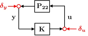
Lemma 2. The interconnection in Figure 2.1 is internally stable if and only if the four closed loop transfer matrices from(δ_y,δ_u)to(u,y)in Figure 2.4 are inRH_∞

(real rational, stable, and proper).

K

y

u

P

22

(33)

C h a p t e r 3

SYSTEM LEVEL PARAMETERIZATION OF STABILIZING

CONTROLLERS

In this chapter, we propose a system level approach to parameterize the set of all internally stabilizing controller. Specifically, we show that the affine subspace defined by the constraints (2.12) - (2.14) parameterizes all stable achievable system responses{R,M,N,L}. In addition, the controllerK=L−MR−1N, which admits a realization as described in (2.15), parameterizes all internally stabilizing controllers for a strictly proper plant P22.1 The results of this chapter provide an alternative

to the traditional Youla parameterization, but is far more amenable for constrained optimal control problems, as will be shown in the next few chapters.

We begin by analyzing the state feedback case, as it admits a simpler characterization and allows us to provide intuition about the construction of a controller that achieves a desired system response. With this intuition in hand, we present our results for the output feedback setting, which is the main focus of this chapter.

3.1 State Feedback

We consider a state feedback problem with plant model given by

P=

      

A B₁ B₂

C₁ D₁₁ D₁₂

I 0 0

      

. (3.1)

The z-transform of the state dynamics (2.1a) is given by

(zI− A)x= B₂u+δx, (3.2)

where we letδx := B1wdenote the disturbance affecting the state.

We defineRto be the system response mapping the external disturbance δx to the statex, andMto be the system response mapping the disturbanceδxto the control actionu. By substituting a dynamic state feedback control ruleu = Kxinto (3.2), we can write the system response{R,M} as a function of the controllerKas

R = (zI− A−B₂K)−1

M = K(zI− A− B₂K)−1.

(34)

The main result of this section is an algebraic characterization of the set {R,M} of state-feedback system responses that are achievable by an internally stabilizing controllerK, as stated in the following theorem.

Theorem 1(System Level Parameterization for State Feedback Systems). For the

state feedback system(3.1), the following are true:

(a) The affine subspace defined by

h

zI− A −B₂

i "

R M

#

= I (3.4a)

R,M ∈ 1

zRH∞ (3.4b)

parameterizes all system responses fromδxto(x,u), as defined in(3.3),

achiev-able by an internally stabilizing state feedback controllerK.

(b) For any transfer matrices{R,M} satisfying(3.4), the controllerK = MR−1is

internally stabilizing and achieves the desired system response(3.3).

The rest of this section is devoted to proving the claims made in Theorem 1.

3.1.1 Necessity

The necessity of a stable and achievable system response{R,M} lying in the affine subspace (3.4) follows from rote calculation. Here we provide some intuition about the conditions (3.4). Note that (3.4a) can be derived by substituting the definition x = Rδx and u = Mδx into (3.2). This condition must hold for any achievable system response(R,M). In addition, for a proper controllerK, the relations in (3.3) imply that bothRandMare strictly proper. Intuitively, the state feedback system (3.2), or the matrix pair (A,B2), is stabilizable if and only if there exists strictly

proper stable transfer matrices R,M ∈ 1_zRH∞ lie in the subspace described by (3.4a). This idea is formally stated and proved by the following lemma.

Lemma 3(Stabilizability). The pair(A,B2)is stabilizable if and only if the affine subspace defined by(3.4)is non-empty.

Proof. We first show that the stabilizability of(A,B2)implies that there exist transfer

(35)

state feedback control lawu = F xinto (3.2), we havex= (zI − A−B2F)

−₁_δ

x and u= F(zI− A−B₂F)−1δ

x. The system response is given byR=(zI− A−B2F)

−₁

andM= F(zI− A−B2F)

−₁

, which lie in 1zRH∞ and are a solution to (3.4a). For the opposite direction, we note that R,M ∈ RH∞ implies that these transfer matrices do not have poles outside the unit circle |z| ≥ 1. From (3.4a), we further observe that

h

zI− A −B₂

i

is right invertible in the region where R and M do not have poles, with

h

R> M>

i>

being its right inverse. This then implies that

h

zI− A −B₂

i

has full row rank for all |z| ≥1. This is equivalent to the PBH test

[15] for stabilizability, proving the claim.

Thus Lemma 3 provides an alternative definition of (state feedback) stabilizability via the conditions described in (3.4) — in particular, stable achievable responses exist only if the state feedback system is stabilizable.

The necessity of conditions (3.4) is provided in the following lemma.

Lemma 4(Necessity of conditions (3.4)). Consider the state feedback system(3.1).

Let(R,M)be the system response achieved by an internally stabilizing controller

K. Then,(R,M)is a solution of (3.4).

Proof. See Appendix 3.A in the end of this chapter.

3.1.2 Sufficiency

Here we show that for any system response {R,M} lying in the affine subspace (3.4), we can construct an internally stabilizing controllerKthat leads to the desired system response (3.3).

A partial solution is provided in our prior work [71], where we give a construction for finite impulse response (FIR) system responses {R,M}. Here we extend these results to infinite impulse response (IIR) system responses, and provide a proof of internal stability for the proposed controller structure.

(36)

proposed the following disturbance-based controller implementation: ˆ

δx[t]= x[t] − xˆ[t] (3.5a)

u[t]= T−₁

Õ

τ=0

M[τ+₁]δˆ_x[t−τ] _(3.5b)

ˆ

x[t+1]= T−₂

Õ

τ=0

R[τ+₂]δˆ_x[t−τ]. _(3.5c)

The internal states of the controller (3.5) should be interpreted as follows: δˆx is the controller estimate of the state disturbance, and ˆxis a desired or reference state trajectory. The estimated disturbance ˆδx[t] is computed by taking the difference between the current state measurement x[t] and the current reference state value

ˆ

x[t]. The control action u[t] and the next reference state value ˆx[t+ 1] are then computed using past estimated disturbances ˆδx[t−T+1], . . . ,δˆx[t].

Taking the z-transform of equations (3.5), we obtain their representation in the frequency domain

ˆ

δx =x− ˆx (3.6a)

u= zM ˆδx (3.6b)

ˆx =(zR−I)δˆ_x. _(3.6c)

Combining equations (3.6) with (3.2) and (3.4), one can verify that the estimated disturbance ˆδx[t] indeed reconstructs the true disturbance δx[t −1]that perturbed the plant at timet −1; hence δˆx = z−1δx. It is then straightforward to show that the desired system response{R,M}satisfyingx = Rδx andu = Mδx is achieved. Note that the previous argument holds for any FIR horizonT as well as forT = ∞. Remark 2. From (3.6), the control action u can be expressed as u = MR−1x.

We can therefore also implement the controller defined in (3.6) via the dynamic

state feedback gain K = MR−1_.₂ _{However, we argue that the disturbance-based} implementation in(3.6)has significant advantages over a traditional state feedback

implementation — specifically, this implementation allows us to connect constraints imposed on the system response to constraints on the controller implementation.

The implementation(3.6) is the key to make a localized linear quadratic regulator

(LLQR) optimal controller (cf., Chapter 5) scalable to implement.

(37)

B

2

1 /z

A

K

R

˜

M

y

x

u

x

u

ˆ

x

P

22

ˆ

_x

Figure 3.1: The proposed state feedback controller structure, withR˜ = I −zRand ˜

M= zM.

It remains to be shown that the controller implementation (3.6) internally stabilizes the plant (3.1). We consider the block diagram shown in Figure 3.1, where here

˜

R = I − zR _and M˜ = zM_{. It can be checked that} R˜ = I − zR = −AR− B₂M ∈ 1

zRH∞ andM˜ = zM ∈ RH∞, and hence the internal feedback loop betweenδˆx

and the reference state trajectory ˆxis well defined.

As is standard, we introduce external perturbations δx,δy, andδu into the system and note that the perturbations entering other links of the block diagram can be expressed as a combination of(δx,δy,δu)being acted upon by some stable transfer matrices.3 Therefore, the standard definition of internal stability applies, and we can use a bounded-input bounded-output argument (e.g., Lemma 2 in Appendix 2.A) to conclude that it suffices to check the stability of the nine closed loop transfer matrices from perturbations (δx,δy,δu) to the internal variables(x,u,δˆx)to determine the internal stability of the structure as a whole.

As all blocks in Figure 3.1 are stable filters, it follows that if the origin(x,δˆx)= (0,0) is asymptotically stable then any other signals in the block diagram will decay asymptotically. This is equivalent to the conventional notion of internal stability [81], which we recall here for the reader before stating and proving that the proposed controller implementation is internally stabilizing.

Definition 4. The interconnection in Figure 3.1 is internally stable if the origin

(x,δˆ_x)=(₀,₀)is asymptotically stable, i.e.,x[t],δˆ_x[t] →₀fort → ∞for all initial

(38)

conditions when the external perturbationsδx, δy, δuin Figure 3.1 are set to0. Lemma 5 (Sufficiency of conditions (3.4)). Consider the state feedback system (3.1). Given any system response{R,M} lying in the affine subspace described by (3.4), the state feedback controllerK= MR−1, with structure shown in Figure 3.1,

internally stabilizes the plant. In addition, the desired system response, as specified

byx= Rδx andu=Mδx, is achieved.

Proof. We first note that from Figure 3.1, we can express the state feedback controller KasK=M(I−˜ R)˜ −1= (zM)(zR)−1 =MR−1. Now, for any system response{R,M} lying in the affine subspace described by (3.4), we construct a controller using the structure given in Figure 3.1. To show that the constructed controller internally stabilizes the plant, we list the following equations from Figure 3.1:

zx= Ax+ B₂u+δx (3.7a)

u= M ˆ˜ δx+δu (3.7b)

ˆ

δx = x+δy+R ˆ˜δx. (3.7c)

Routine calculations (see Appendix 3.A for details) show that the closed loop transfer matrices from(δx,δy,δu)to(x,u,δˆx)are given by

       x u ˆ δx        =       

R −R˜ −RA RB₂

M M˜ −MA I+MB₂

1

zI I− 1zA 1zB2               δx δy δu        . (3.8)

As all nine transfer matrices in (3.8) are stable, the implementation in Figure 3.1 is internally stable. Furthermore, the desired system response {R,M}, from δx to

(x,u)_{, is achieved.}

3.1.3 Summary and corollary

The proof of Theorem 1 is then straightforward.

Proof of Theorem 1. The statements follow directly by combining the results of

Lemma 4 and 5.

(39)

We note that the analysis for the state feedback problem can be applied to the state estimation problem by considering the dual to a full control system (c.f., §16.5 in [81]). For instance, the following corollary to Lemma 3 gives an alternative definition of the detectability of pair(A,C2)[74].

Corollary 1(Detectability). The pair(A,C2)is detectable if and only if the following conditions are feasible:

h

R N

i "

zI− A −C₂

#

= I (3.9a)

R,N∈ 1

zRH∞. (3.9b)

A parameterization of all detectable observers can be constructed using the affine subspace (3.9) in a manner analogous to that described above. We will give a more detailed discussion about state estimation application in Section 5.6.

Finally, we note that Theorem 1 can be extended to continuous time system imme-diately by replacingz-transform variablezto the Laplace transform variables. The corollary of Theorem 1 for continuous time system is therefore given as follows: Corollary 2_{(Theorem 1 for continuous time systems)}. For a continuous time state feedback system with state space realization_(3.1), the following are true:

(a) The affine subspace defined by

h

sI− A −B₂

i "

R M

#

= I (3.10a)

R,M∈ 1

sRH∞ (3.10b)

parameterizes all system responses fromδxto(x,u)achievable by an internally stabilizing state feedback controllerK.

(b) For any transfer matrices {R,M} satisfying(3.10), the controllerK = MR−1

is internally stabilizing and achieves the desired system responsex=Rδxand

(40)

3.2 Output Feedback for Strictly Proper Systems

We now extend the arguments of the previous section to the output feedback setting, and begin by considering the case of a strictly proper plant

P=

      

A B₁ B₂ C₁ D₁₁ D₁₂ C₂ D₂₁ 0

      

. (3.11)

Letting δx[t] = B₁w[t] denote the disturbance on the state, and δy[t] = D21w[t]

denote the disturbance on the measurement, the dynamics defined by plant (3.11) can be written as

x[t+1] = Ax[t]+B2u[t]+δx[t]

y[t] = C₂x[t]+δ_y[t]. _(3.12)

Analogous to the state-feedback case, we define a system response{R,M,N,L}from perturbations(δx,δy)to state and control inputs(x,u)via the following relation:

"

x u

# =

"

R N

M L

# "

δx

δy #

. (3.13)

Substituting the output feedback control lawu= Kyinto the z-transform of system equation (3.12), we obtain

(zI− A−B₂KC₂)x= δx+B2Kδy.

For a proper controller K, the transfer matrix (zI − A− B2KC2) is always

invert-ible because its leading coefficient zI is invertible, hence we obtain the following expressions for the system response (3.13) in terms of an output feedback controller K:

R=(zI− A−B₂KC₂)−1

M=KC₂R

N=RB₂K

L=K+KC₂RB₂K. _(3.14)

(41)

Theorem 2 (System Level Parameterization for Output Feedback Systems with Strictly Proper Plants). For the output feedback system (3.11), the following are

true:

(a) The affine subspace described by:

h

zI− A −B₂

i "

R N

M L

#

= hI 0

i

(3.15a)

"

R N

M L

# "

zI −A −C₂

# =

"

I

0

#

(3.15b) R,M,N∈ 1

zRH∞, L ∈ RH∞ (3.15c)

parameterizes all system responses_(3.14)achievable by an internally stabilizing controllerK.

(b) For any transfer matrices {R,M,N,L} satisfying (3.15), the controller K = L−MR−1_N_{is internally stabilizing and achieves the desired response}_(3.14)_.

As the equations (3.15a) - (3.15c) characterize the set of all stable and achievable system responses, we call it a system level parameterization (SLP).

3.2.1 Necessity

As was the case for the state-feedback setting, the necessity of a stable and achievable system response {R,M,N,L} lying in the affine subspace (3.15) follows from rote calculation. We first provide some intuition about how the equality constraints (3.15a) - (3.15b) are derived from the relations (3.14). Using the identity (zI − A− B₂KC₂)R = I and the relation M = KC2R, we get (zI − A)R − B2M = I.

Likewise, we have the relation (zI − A)N − B2L = 0. Therefore, the system

response must satisfy the equality constraint in (3.15a). Similarly, using the identity R(zI−A−B₂KC₂)= I, we know that the system response must also satisfy (3.15b). Besides, from the relations in (3.14), we note that R,M, and N must be strictly proper, and all the system response are stable becauseKis an internally stabilizing controller. This leads to the constraint (3.15c). Intuitively, the equations (3.15a) -(3.15c) are feasible as long as the system matrices(A,B2)is stabilizable and(A,C2)

is detectable. This is formally stated in the following lemma.

(42)

Lemma 6 provides an alternative characterization of stabilizability and detectability via the conditions described in (3.15) — in particular, stable achievable system re-sponses (3.14) exist only if the output feedback system is stabilizable and detectable. The next lemma shows that (3.15) is a necessary condition for the system response to be stable and achievable.

Lemma 7 (Necessity of conditions (3.15)). Consider the output feedback system (3.11). Let {R,M,N,L}, with x = Rδx + Nδy and u = Mδx + Lδy, be the system response achieved by an internally stabilizing control law u = Ky. Then,

{R,M,N,L} lies in the affine subspace described by(3.15).

3.2.2 Sufficiency

B

2

1 /z

A

1 /z

C

2

y

x

u

x

u

y

˜

M

L

˜

N

˜

R

+

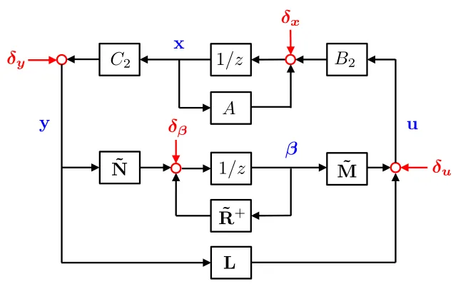
Figure 3.2: The proposed output feedback controller structure, with R˜+ = zR˜ = z(I−zR),M˜ = zM, andN˜ =−zN.

Here we show that for any system response{R,M,N,L}lying in the affine subspace (3.15), there exists an internally stabilizing controller K that leads to the desired system response (3.14). From the relations in (3.14), we notice the identity K = L−KC₂RB₂K= L−MR−1_N

A System Level Approach to Optimal Controller Design for Large-Scale Distributed Systems

for Large-Scale Distributed Systems

Yuh-Shyang Wang

ACKNOWLEDGEMENTS

ABSTRACT

PUBLISHED CONTENT AND CONTRIBUTIONS

TABLE OF CONTENTS

LIST OF ILLUSTRATIONS

LIST OF TABLES

INTRODUCTION

K

P

x

[

t

+ 1] =

Ax

[

t

] +

B

u

[

t

] +

[

t

]

y

[

t

] =

C

x

[

t

] +

[

t

]

⇠

[

t

+ 1] =

A

⇠

[

t

] +

B

y

[

t

]

u

[

t

] =

C

⇠

[

t

] +

D

y

[

t

]

y

u



x

u



PROBLEM STATEMENT AND MAIN RESULTS

P

P

P

P

K

_u