A Clustering Algorithm for Classification of
Network Traffic using Semi Supervised Data
Anjali Wankhede Kailash Patidar
M. Tech Scholar Head of Dept.
Department of Computer science & Engineering Department of Computer science & Engineering Sri Satya Sai Institute of Scienec & Technology Sehore (M.P.) Sri Satya Sai Institute of Scienec & Technology Sehore (M.P.)
Abstract
In traditional text classification, a classifier is built using supervised training documents of every class. This paper studies a different problem. Given a set P of documents of a particular class (called positive class) and a set U of unsupervised documents that contains documents from class P and also other types of documents (called negative class), we want to build a classifier to classify the documents in U into documents from P and documents not from P. The key feature of this problem is that there is no supervised negative document, which makes traditional text classification techniques inappropriate. So In this paper, we propose an effective technique to solve the problem. It combines the Rocchio method and the K-means technique for classifier network data. Experimental results show that the new method outperforms existing methods significantly.
Keywords: supervised data, labeled data, clustering, K-means, network traffic, classification
_______________________________________________________________________________________________________
I. INTRODUCTION
Text classification is a main problem and has been studied extensively in information fetched and machine learning. To build a text classifier, the user first collects a set of training examples, which are labeled with pre-defined classes (labeling work is often done manually). A clustering algorithm is then applied to the training data to build a classifier. This approach to building classifiers is called supervised classification because the training examples/documents all have pre-labeled classes.
This paper studies a special form of semi-supervised text classification. This problem can be regarded as a two -class (positive and negative) classification problem, where there are only supervised positive training data, but unsupervised negative training data. Due to the lack of negative training data, the classifier building is thus semi-supervised. Since traditional classification techniques require both labeled positive and negative examples to build a classifier, they are thus not suitable for this problem. Although it is possible to manually label some negative examples, it is labor-intensive and very time consuming. In this paper, we want to make a classifier using only a set of positive examples and a set of unsupervised examples. Collecting unlabeled examples or documents is normally easy and inexpensive in many text or Web page domains, especially those involving online sources [Nigam et al., 1998; Liu et al., 2014].
In [Liu et al., 2014; Yu et al., 2014], two techniques are proposed to solve the problem. One is based on the EM al-gorithm [Dempster et al., 1977] (called S-EM) and the other is based on Support Vector Machine (K-means) [Vapnik, 1995] (K- mediods). However, both techniques have some major shortcomings. K -means is not accurate because of its weak classifier.K-mediods is not robust because it performs well in certain situations and fails badly in others. We will discuss these two techniques in detail in Section 2 and compare their results with the proposed technique in Section 4.
As discussed in our earlier work [Liu et al., 2014], positive class based learning occurs in many applications. With the growing volume of text documents on the Web, Internet news feeds, and digital libraries, one often wants to find those documents that are related to one’s interest. For instance, one may want to build a repository of ma-chine learning (ML) papers. One can start with an initial set of ML papers (e.g., an ICML Proceedings). One can then find those ML papers from related online journals or conference series, e.g., AI journal, AAAI, IJCAI, etc.
The ability to build classifiers without negative train-ing data is particularly useful if one needs to find positive documents from many text collections or sources. Given a new collection, the algorithm can be run to find those positive documents. Following the above example, given a collection of AAAI papers (unlabeled set), one can run the algorithm to identify those ML papers. Given a set of SIGIR papers, one can run the algorithm again to find those ML papers. In general, one cannot use the classifier built using the AAAI collection to classify the SIGIR collection because they are from different domains. In traditional classification, labeling of negative documents is needed for each collection. A user would obviously prefer techniques that can provide accurate classification without manual labeling any negative documents.
II. LITERATURE SURVEY
Many studies on text clustering have been conducted in the past. Present algorithms like Bayes (NB), K-means, and many others. These existing techniques, how-ever, all require supervised training data of all classes. They are not designed for the positive class based clustering.
In [Denis, 1998], a theoretical study of PAC learning from positive and unlabeled examples under the statistical query model [Kearns, 1998] is reported. [Letouzey et al., 2000] presents an algorithm for learning using a modified decision tree algorithm based on the statistical query model. It is not for text classification, but for normal data. In [Muggleton, 2014], Muggleton studied the problem in a Bayesian framework where the distribution of functions and examples are assumed known. The result is similar to that in [Liu et al., 2014] in the noiseless case. [Liu et al., 2014] extends the result to the noisy case. The purpose of this paper is to propose a robust practical method to im-prove existing techniques.
In [Liu et al., 2014], Liu et al. proposed a method (called S- EM) to solve the problem in the text domain. It is based on naïve Bayesian classification (NB) and the EM algorithm [Dempster et al., 1977]. The main idea of the method is to first use a spy technique to identify some reliable negative documents from the unlabeled set. It then runs EM to build the final classifier. Since NB is not a strong classifier for texts, we will show that the proposed technique is much more accurate than S-EM.
In [Yu et al., 2014], Yu et al. proposed a SVM based technique (called PEBL) to classify Web pages given positive and unlabeled pages. The core idea is the same as that in [Liu et al., 2014], i.e., (1) identifying a set of re-liable negative documents from the unlabeled set (called strong negative documents in PEBL), and (2) building a classifier using SVM. The difference between the two techniques is that for both steps the two techniques use different methods. In [Yu et al. , 2014], strong negative documents are those documents that do not contain any features of the positive data. After a set of strong negative documents is identified, SVM is applied iteratively to build a classifier. PEBL is sensitive to the number of positive examples. When the positive data is small, the results are often very poor. The proposed method differs from PEBL in that we perform negative data extraction from the unlabeled set using the Rocchio method and clustering. Although our second step also runs SVM it-eratively to build a classifier, there is a key difference. Our technique selects a good classifier from a set of classifiers built by SVM, while PEBL does not. The proposed method performs well consistently under a variety of conditions.
In [Scholkopf et al., 1999], one-class SVM is proposed. This technique uses only positive data to build a SVM classifier. However, our experiment results show that its classification performance is poor.
Another line of related work is the use of a small labeled set of every class and a large unlabeled set for learning [Ni-gam et al., 1998; Blum & Mitchell, 1998; Goldman & Zhou, 2014; Basu et al., 2015; Muslea et al., 2014; Bockhorst & Craven, 2014]. It has been shown that the unlabeled data helps classification. This is different from our work, as we do not have any labeled negative training data.
III. THE PROPOSED ALGORITHM
This section presents the proposed approach, which also consists of two steps: (1) extracting some reliable negative documents from the unlabeled set, (2) applying SVM iteratively to build a classifier. Below, we present these two steps in turn. In Section 4, we show that our technique is much more robust than existing techniques.
Finding reliable negative documents
This sub-section gives two methods for finding reliable negative documents: (1) Rocchio and (2) Rocchio with clustering. The second method often results in better classi-fiers, especially when the positive set is small. The key re-quirement for this step is that the identified negative docu-ments from the unlabeled set must be reliable or pure, i.e., with no or very few positive documents, because SVM (used in our second step) is very sensitive to noise.
Method 1: Rocchio
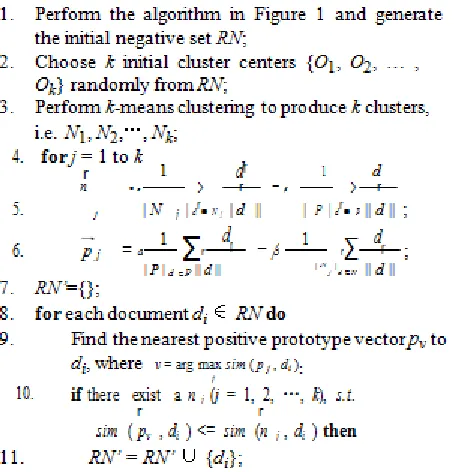
This method treats the entire unlabeled set U as negative documents and then uses the positive set P and U as the training data to build a Rocchio classifier. The classifier is then used to classify U. Those documents that are classified as negative are considered (reliable) negative data, denoted by RN. The algorithm is shown in Figure 1.
In Rocchio classification, each document d is represented as a vector [Salton & McGill, 1983], d = (q1 , q2 ,L, qn ). Each element qi in d represents a word wi and is calculated as the combination of term frequency (tf) and inverse document frequency (idf), i.e., qi = tfi * idfi. tfi is the number of times that word wi occurs in d, while
idf i = log(| D | / df (wi )) .
Here |D | is the total number of documents and df(wi) is the number of documents where word wi occurs at least once.
Building a classifier is achieved by constructing positive− (lines 2 and 3 inand negative prototype vectorscr+ and cr Figure 1).
α and β parameters adjust the relative impact of positive and negative training examples. α = 16 and β = 4 are recommended in [Buckley et al., 1994].
In classification, for each test document d ' , it simply uses the cosine measure [Salton & McGill, 1983] to compute the similarity (sim) of d ' with each prototype vector. The class whose prototype vector is more similar to d ' is assigned to the test document (lines 4-6 in Figure 1). Those documents classified as negative form the negative set RN.
In general, it is also possible to use other classification methods (e.g., naïve Bayesian, SVM) to extract negative data from the unlabeled set. However, not all classification tech-niques perform well in the absence of a “pure” negative training set. We experimented with SVM, naïve Bayesian and Rocchio, and observed that Rocchio produces the best results. It is able to extract a large number of true negative documents from U with very high precision.
The reason that Rocchio works well is as follow: In our positive class based learning, the unlabeled set U typically has the following characteristics:
1. The proportion of positive documents in U is very small. Thus, they do not affect r− very much. c
The negative documents in U are of diverse topics. Thus, in the vector space, they cover a very large region.
Since the positive set P is usually homogenous (focusing on one topic), they cover a much smaller region in the vector space. Assume that there is a true decision surface S thatseparates positive and negative data. Then, the positive pro- r+ totype vector c
will be closer to S than the negative proto-r− type vector
c
due to the vector summation in Rocchio (line 2 and 3 of Figure 1).Because of this reason, when we apply the similarity computation (in line 5 of Figure 1) to classify
Documents, many negative documents will be classified aspositive because they are closer to r+ . This explains why c Rocchio
can extract negative documents with high precision, and positive documents with low precision (but very high recall). Our experiments show that this is indeed the case.
After some reliable negative documents are found from U by Rocchio, we can run SVM using P and RN. Experimental results show that this simple approach works very well. Note that we could actually use cr+ and cr in Figure 1 as the final classifier without using SVM. However, it does not perform well because it tends to classify too many negative docu-ments as positive documents (low precision for positive). SVM using RN and P as training data can correct the situa-tion and produce a more accurate final classifier.
Method 2: Rocchio with Clustering
Rocchio is a classifier based on cosine similarity. When the decision boundary is non- linear or does not con-form to the separating plane resulted from cosine similarity, Rocchio may still extract some positive documents and put them in RN. This will damage the K-means classifier later. Be-low, we propose an enhancement to the Rocchio approach in order to purify RN
further, i.e., to discard some likely positive documents from RN.
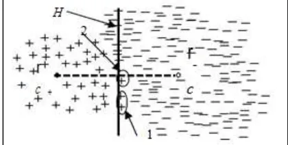
Figure 2 shows a possible scenario where some positive documents in U may still be in RN. cr+ and cr represent thepositive and negative prototype vectors respectively. H is the decision hyperplane produced by Rocchio. It has the same distance (similarity) to c r+ and c r If a document is located on the right-hand-side of H, it is classified as negative oth-erwise it is classified as positive. However, the positive and negative classes in the data cannot be separated by H well. In Figure 2, the positive documents within the regions 1 and 2 will be misclassified as negative documents.
Fig. 2: Rocchio classifier is unable to remove some posi-tive examples in U
In order to further “purify” RN, we need to deal with the above problem. We propose the following approach.
better accuracy. Since both the cluster and the positive set are homogeneous, they allow Rocchio to build better prototype vectors.
The clustering technique that we use is k- means, which is an efficient technique. The k-means method needs the input cluster number k. From our experiments in Section 4, we observe that the choice of k does not affect classification results much as long as it is not too small. Too few clusters may not be effective because the documents in a cluster can still be diverse. Then, Rocchio still cannot build an accurate classifier. Too many clusters will not cause much problem.
This new method can further purify RN without removing too many negative documents from RN. The detailed algo-rithm is given in Figure 3.
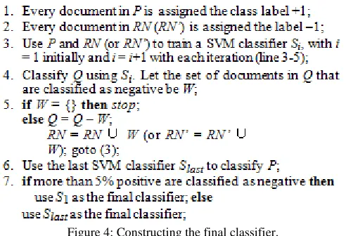
Note that in line 1 we still perform the initial Rocchio extraction as discussed in Section 3.1.1. Thus, the input data for clustering is RN, not U. The reason is that the purity of RN is higher, which allows us to produce better clusters without the influence of too many noisy (positive) documents in U. Lines 2-3 perform the standard k-means clustering of RN, which produces k clusters, N1, N2, …, Nk. Based on these clusters, we construct a positive prototype vector pj and a negative prototype vector n j for the positive set P and each cluster Nj ( j ∈ {1, 2, …, k} (lines 5 and 6). Line 8 starts the extraction. For each document di∈r RN, we try to find the nearest positive prototype vector pv to di (line 9). If the similarity sim( p ,d ) is less than the similarity between di and any negative prototypevi vector nrj , we put it in our final negative set RN’ (line 10). The reason for using the proce-dures in lines 9 and 10 is that we want to be conservative in removing likely positive documents from RN, i.e., not to remove too many negative documents.
Figure 3: Rocchio extraction with clustering.
After RN’ is determined, we can build the final classifier using SVM, which takes P and RN’ as the positive and negative training data respectively.
Step 2: Classifier building
Figure 4: Constructing the final classifier.
The reason that we run SVM iteratively (lines 3-5) is that the reliable negative set RN from step 1 may not be suffi-ciently large to build the best classifier. SVM classifiers (Si in line 3) can be used to iteratively extract more negative documents from Q. The iteration stops when there is no negative document that can be extracted from Q (line 5).
There is, however, a danger in running SVM iteratively. Since SVM is very sensitive to noise, if some iteration of SVM goes wrong and extracts many positive documents from Q and put them in the negative set RN, then the last SVM classifier will be extremely poor. This is the problem with PEBL, which also runs SVM iteratively. In our algo-rithm, we decide whether to use the first SVM classifier or the last one (line 7). Basically, we use the SVM classifier at convergence (called Slast, line 6) to classify the positive set P. If too many (> 5%) positive documents in P are classified as negative, it indicates that SVM has gone wrong. We then use the first SVM classifier (S 1). Otherwise, we use Slast as the final classifier. We choose 5% as the threshold because we want to be very conservative. Since SVM is very sensitive to noise, when noise is large, the resulting classifier is often very poor. Since our first classifier is always quite strong, even without catching the last classifier which may be better, it is acceptable.
Note that this strategy is not applicable to PEBL because PEBL’s step 1 extracts too few negative documents from U. Its first SVM classifier is thus very inaccurate. Step 1 of our proposed technique is able to extract a large number of negative documents from U. Hence, our first SVM classifier is always quite good, although it may not be the best.
Note also that neither the first nor the last SVM classifier may be the best. This is the case for both PEBL and our algorithm. In many cases, a classifier somewhere in the middle is the best. However, it is hard to catch it. We leave this issue to our future research.
IV. EMPIRICAL EVALUATION
This section evaluates the proposed techniques using the Reuters-21578 text collection1, which is commonly used in evaluating text classification methods. We will also compare the proposed techniques with S-EM and PEBL.
The Reuters- 21578 collection contains 21578 text docu-ments. We used only the most populous 10 out of the 135 topic categories. Table 1 gives the number of documents in each of the ten topic categories. In our experiments, each category is used as the positive class, and the rest of the categories as the negative class. This gives us 10 datasets.
Table 1: Categories and numbers of documents in Reuters acq corn crude earn grain interest money ship trade wheat
2369 238 578 3964 582 478 717 286 486 283
Our task is to identify positive documents from the unlabeled set. The construction of each dataset for our experiments is done as follows: Firstly, we randomly select a% of the documents from the positive class and the negative class, and put them into P and N classes respectively. The remaining (1 - a %) documents from both classes form the unlabeled set U. Our training set for each dataset consists of P and U. N is not used as we do not want to change the class distribution of the unlabeled set U. We also used U as the test set in our experiments because our objective is to recover those positive documents in U. We do not need separate test sets. In our experiments, we use 7 a values to create different settings, i.e., 5%, 15%, 25%, 35%, 45%, 55% and 65%.
Evaluation Measures:
on the other hand, reflects an average effect of both precision and recall. This is suitable for our purpose, as we want to identify posi-tive documents. It is undesirable to have either too small a precision or too small a recall.
In our experimental results, we also report accuracies. It, however, should be noted that accuracy does not fully reflect the performance of our system, as our datasets has a large proportion of negative documents. We believe this reflects realistic situations. In such cases, the accuracy can be high, but few positive documents may be identified.
Experimental Results:
We now present the experimental results. We use Roc-SVM and Roc-Clu-SVM to denote the classification techniques that employ Rocchio and Rocchio with clustering to extract reliable negative set respectively (both methods use SVM for classifier building). We observe from our experiments that using Rocchio and Rocchio with clustering alone for classi-fication do not provide good classification results. SVM improves the results significantly.
For comparison, we include the classification results of NB, S-EM and PEBL. Here, NB treats all the documents in the unlabeled set as negative. SVM for the noisy situation (U as negative) performs poorly because SVM does not tolerate noise well. Thus, its results are not listed (in many cases, its F values are close to 0). In both Roc-SVM and Roc-Clu-SVM, we used the linear SVM as [Yang & Liu, 1999] reports that linear SVM gives slightly better results than non-linear models on the Reuters dataset. For our experiments, we im-plemented PEBL as it is not publicly available. For SVM, we used the SVMlight system [Joachims, 1999]. PEBL also used SVMlight. S-EM is our earlier system. It is publicly available at http://www.cs.uic.edu/~liub/S-EM/S-EM-download.html. Table 2 shows the classification results of various tech-niques in terms of F value and accuracy (Acc) for a = 15% (the positive set is small). The final row of the table gives the average result of each column. We used 10 clusters (i.e., k = 10) for k-means clustering in Roc-Clu -SVM (later we will see that the number of clusters does not matter much).
We observe that Roc-Clu-SVM produces better results than Roc- SVM. Both Roc-SVM and Roc-Clu-SVM outper-form NB, S-EM and PEBL. PEBL is extremely poor in this case. In fact, PEBL performs poorly when the number of positive documents is small. When the number of positive documents is large, it usually performs well (see Table 3 with = 45%). Both Roc-SVM and Roc-Clu-SVM perform well consistently. We summarize the average F value results of all
settings
in Figure 5. Due to space limitations, we are unable to show the accuracy results (as noted earlier, accuracy does not fully reflect the performance of our system).Table – 2
Experiment results for a = 15%.
15% NB S-EM PEBL Roc-SVM Roc-Clu-SVM
acq F Acc F Acc F Acc F Acc F Acc
0.744 0.920 0.876 0.954 0.001 0.817 0.846 0.948 0.867 0.952 corn 0.452 0.983 0.452 0.983 0.000 0.982 0.804 0.993 0.822 0.995 crude 0.731 0.979 0.820 0.984 0.000 0.955 0.782 0.983 0.801 0.985 earn 0.910 0.949 0.947 0.968 0.000 0.693 0.858 0.924 0.891 0.959 grain 0.728 0.977 0.807 0.982 0.020 0.955 0.845 0.987 0.869 0.986 interest 0.609 0.972 0.648 0.970 0.000 0.963 0.704 0.976 0.724 0.983 money 0.754 0.974 0.793 0.975 0.000 0.945 0.768 0.973 0.785 0.973 ship 0.701 0.989 0.742 0.990 0.008 0.978 0.578 0.986 0.596 0.989 trade 0.627 0.977 0.698 0.979 0.000 0.962 0.759 0.983 0.778 0.985 wheat 0.579 0.982 0.611 0.979 0.000 0.978 0.834 0.994 0.854 0.997 Avg 0.684 0.970 0.739 0.976 0.003 0.923 0.778 0.975 0.799 0.980
Table – 3
Experiment results for a = 45%.
45% NB S-EM PEBL Roc-SVM Roc-Clu-SVM
acq F Acc F Acc F Acc F Acc F Acc
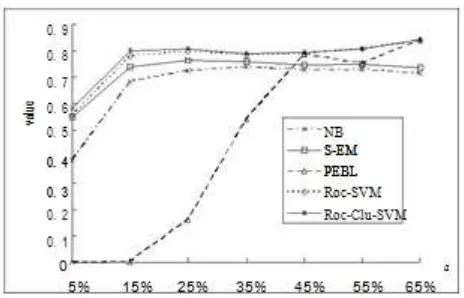
Fig. 5: Average results for all a setting from Figure 5, we can draw the following conclusions:
1) S-EM’s results are quite consistent under different set-tings. However, its results are worse than Roc-SVM and Roc-Clu-SVM. The reason is that the negative documents extracted from U by its spy technique are not that reliable, and S-EM uses a weaker classifier, NB.
2) PEBL’s results are extremely poor when the number of positive documents is small. We believe that this is be-cause its strategy of extracting the initial set of strong negative documents could easily go wrong without suf-ficient positive data. Even when the number of positive documents is large, it may also go wrong. For example, for a = 55%, one F value (for the dataset, trade) is only 0.073. This shows that PEBL is not robust.
3)
Both Roc-SVM and Roc-Clu-SVM are robust with dif-ferent numbers of positive documents. This is important because in practice one does not know how many positive documents are sufficient. Using a smaller set of positive documents also reduce the manual labeling effort.From Figure 5, we also observe that Roc-Clu-SVM is slightly better than Roc-SVM in both F value and accu-racy, especially when a is small because pure RN is more important in such cases. When a is large, their results are similar. In practice, Roc-SVM may be sufficient due to its simplicity, efficiency and good results.
We also ran one-Class SVM using the LIBSVM package (http://www.csie.ntu.edu.tw/~cjlin/libsvm/). It gives very poor results (mostly with F values less than 0.4). Due to space limitations, we do not list their results here.
Comparison of different number of clusters: As discussed above, the number of clusters used in Roc-Clu-SVM makes little difference to the final classifier. We now provide ex-periment results in Figure 6 to support this claim by using different numbers of clusters (here, a = 25% and for other a values, the results are similar). The cluster number k varies from 2 to 30. We observe that the choice of k has little in-fluence on the results as long as it is not too small.
Fig. 6: Averaged F values of different clusters (a=25%)
Execution times: Our technique consists of two steps: ex-tracting negative documents from U and iteratively running SVM. As SVM is a standard technique, we will not discuss it here. If we only use Rocchio for the first step, it is very effi-cient because Rocchio is a linear algorithm, O(|U∪P|). If we use Rocchio with clustering, more time is needed because of k-means clustering. The time complexity of k-means is O(k*|RN|* I), where k is the number of clusters, |RN| is the size of the reliable negative set, and I is the number of itera-tions. Since k and I are normally small, k-means is generally regarded as a linear algorithm O(|RN|). Thus, the time com-plexity of the extraction step of Roc-Clu-SVM is O(|U∪P|) since |RN| < |U∪P|. In our experiments, every dataset takes less than 7 seconds for step one for Roc-Clu-SVM (on Pen-tium 800MHz PC with 256MB memory).
ACKNOWLEDGEMENT
This research is supported by a researchgrant from A-STAR and NUS to the second author. REFERENCES
[1] [Basu et al., 2015] S. Basu, A. Banerjee, & R. Mooney. Semi-supervised clustering by seeding. ICML-2015 [2] [Blum & Mitchell, 2014] A. Blum & T. Mitchell. Combining labeled & unlabeled data with co-training. COLT-2014.
[3] [Bockhorst & Craven, 2014] J. Bockhorst & M. Craven. Exploiting relations among concepts to acquire weakly labeled training data. ICML-2014. [4] [Buckley et al., 2014] C. Buckley, G. Salton, and J. Allan. The effect of adding relevance information in a relevance feedback environment. SIGIR-2014. [5] [Dempster et al., 1977] A. Dempster, N. Laird & D. Rubin. Maximum likelihood from incomplete data via the EM algorithm. Journal of the Royal
Statistical Society, 1977.
[6] [Denis, 1998] F. Denis. PAC learning from positive statisti-cal queries. ALT-98, pages 112-126. 1998.
[7] [Goldman & Zhou, 2014] S. Goldman & Y. Zhou. Enhancing supervised learning with unlabeled data. ICML-2014
[8] [Joachims, 1999] T. Joachims. Making large-Scale SVM Learning Practical. Advances in Kernel Methods - Support Vector Learning, B. Schölkopf and C. Burges and A. Smola (ed.), MIT-Press, 1999
[9] [Kearns, 1998] M. Kearns. Efficient noise-tolerant learning from statistical queries. J. of the ACM,45:983-1006, 1998.
[10] [Letouzey et al., 2014] F. Letouzey, F. Denis, R. Gilleron, & E. Grappa. Learning from positive and unlabeled exam-ples. ALT-00, 2014. [11] [Lewis & Gale, 1994] D. Lewis & W. Gale. A sequential algorithm for training text classifiers. SIGIR-94, 1994.
[12] [Liu et al., 2014] B. Liu, W. Lee, P. Yu, & X. Li. Partially supervised classification of text documents. ICML-2002.
[13] [Muslea et al., 2014] I. Muslea, S. Minton & C. Knoblock. Active + semi-supervised learning = robust multi-view learning. ICML-2014. [14] [Muggleton, 2014] S. Muggleton. Learning from the positive data. Machine Learning, 2014, to appear.
[15] [Nigam et al., 1998] K. Nigam, A. McCallum, S. Thrun, & T. Mitchell. Text classification from labeled and unlabeled documents using EM, machine learning, 1999.
[16] [Rocchio, 1971] J. Rocchio. Relevant feedback in informa-tion retrieval. In G. Salton (ed.). The smart retrieval sys-tem: experiments in automatic document processing, Englewood Cliffs, NJ, 1971.
[17] [Salton & McGill, 1983] G. Salton & M. McGill. Introduc-tion to Modern Information Retrieval. McGraw-Hill,1983.
[18] [Scholkopf et al., 1999] B. Scholkopf, J. Platt, J. Shawe, A. Smola & R. Williamson. Estimating the support of a high-dimensional distribution. Technical Report MSR-TR-99-87, Microsoft Research, 1999.
[19] [Vapnik, 1995] V. Vapnik. The nature of statistical learning theory, 1995.
[20] [Yang & Liu, 1999] Y. Yang & X. Liu. A re-examination of text categorization methods. SIGIR-99, 1999.