A Comparative study on Algorithms for Shortest-Route Problem and Some
Extensions
Sohana Jahan, Md. Sazib Hasan
Abstract-- The shortest-route problem determines shortest routes from one node to another. In this paper Dijkstra’s Algorithm and Floyd’s algorithm to determine shortest route between two nodes in the network are discussed. Some extensions in Floyd’s algorithm have done. We have formulated a shortest route problem as a linear programming problem and solved it as a 0-1 integer programming problem. The dual of the formulated linear programming problem is also used to determine the shortest routes. Complementary Slackness Theorem is used to solve the primal problem from the solution of the dual problem and to determine the shortest distance as well as the shortest routes.
Index Terms-- Complementary Slackness Theorem, Dual of an LPP, Dijkstra’s algorithm, Floyd’s algorithm, 0-1 Integer Programming Problem.
I. Introduction
etwork optimization [7], [13] has always been at the heart of operational research. Shortest Route model is one of the network models whose applications cover a wide range of areas,
such as telecommunications and
transportation planning. The shortest-route problem [2],[4],[6] determines shortest routes from one node to another. There are a number of algorithms that can be used to
Sohana Jahan is with the the Department of Mathematics, University of Dhaka, Dhaka, Bangladesh
( e-mail:[email protected])
Md. Sazib Hasan is with the Department of Mathematics, Brac University , Dhaka, Bangladesh. (e-mail : [email protected])
determine shortest distance and shortest route between two nodes in a network. In this paper we have discussed Dijkstra’s algorithm [1], [6] and Floyd’s algorithm [4]. We have made some extensions in Floyd’s algorithm. We have given the linear programming formulation of a shortest route problem and solved it as a 0-1 integer programming problem [4]. We have also solved the problem by solving the dual of the formulated linear programming problem [3] and determined the shortest routes. We have also used Complementary Slackness Theorem [5] to solve the primal problem from the solution of the dual problem and determined the shortest distance as well as the shortest routes.
II. Algorithms to find Shortest-Route
There are a number of algorithms that can be used to determine shortest route between two nodes in a network. Among them Dijkstra’s algorithm and Floyd’s algorithm are more efficient. Dijkstra’s algorithm [1],[6] determines the shortest route between the source node and every other node and Floyd’s algorithm[4] determines the shortest route between all pair of nodes in the network.
2.1 Dijkstra’s algorithm:
Let ui be the shortest distance from source
node 1 to node i, and define dij (≥ 0)as the
length of arc (i, j). Then the algorithm
defines the label for an immediately succeeding node j as
[ui, i] = [ui + dij, i], dij≥ 0.
The label for the starting node is [0, -], indicating that the node has no predecessor. Node labels in Dijkstra’s algorithm are of two types: temporary and permanent. A temporary label is modified if a shorter route to a node can be found. At the point when no better routes can be found, the status of
the temporary label is changed to
permanent.
Step 0: Label the source node (node 1) with
the permanent label [0, - ]. Set i = 1,
Step i: (a) Compute the temporary labels
[ui + dij ,i] for each node j that can be
reached from node i, provided j is not permanently labeled. If node j is already
labeled with [uj, k] through another node k
and if ui + dij < uj, replace [uj, k] with
[ui + dij, i].
(b)If all the nodes have permanent labels,
stop. Otherwise, select the label [ur, s]
having the shortest distance (= ur) among all
the temporary labels. Set i = r and repeat step i.
Now we consider the following network to implement the Dijkstra’s algorithm
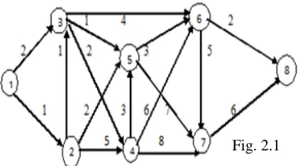
Example: The network in Fig: 2.1 gives the
routes and their lengths in miles between city 1(node 1) and seven other cities (nodes 2, 3, 4, 5, 6, 7, 8). We determine the shortest routes between city 1 and each of the remaining seven cities.
According to Dijkstra’s algorithm we start with iteration 0.
Iteration 0: Assign the permanent label
[0,-] to node 1.
Iteration 1: Nodes 2 and 3 can be reached
from node 1. Thus, the list of labeled nodes (temporary and permanent) becomes
Node Label Status
1 [0, -] Permanent
2 [0+1, 1]=[1,1] Temporary
3 [0+2, 1]=[2,1] Temporary
Between the two temporary labels [1, 1] and [2, 1], node 2 yields the smaller distance
(u2=1). Thus, the status of node 2 is changed
to permanent.
Iteration 2: Nodes 4 and 5 can be reached
from node 2, and the list of labeled nodes becomes
Node Label Status
1 [0,-] Permanent
2 [1,1] Permanent
3 [2,1] or
[1+1,2]=[2,2]
Temporary
4 [1+5,2]=[6, 2] Temporary
5 [1+2, 2] = [3, 2] Temporary
Among the temporary labels [2, 1], [6, 2], [3, 2], node 3 yields the smaller distance
(u3=2). Thus, the status of the temporary
label [2, 1] at node 3 is changed to permanent.
Continuing in this way we have the final table in the last iteration:
Iteration 8:
Node Label Status
1 [0,-] Permanent
2 [1,1] Permanent
3 [2, 1] Permanent
4 [4, 3] Permanent
5 [3, 2] , [3, 3] Permanent
6 [6, 3] or [6, 5] Permanent
7 [10,5] Permanent
8 [8, 6] Permanent
Therefore, the following sequence
determines the shortest route from node 1 to node 8
(8) → [8, 6] → (6) → [6, 5 ] → (5) → [3, 3]
→(3) →[2,1] → (1)
Thus, the required rout is 1→ 3 →5 → 6 → 8
with a total length of 8 miles.
The route is shown in the following diagram in blue color.
The alternative routes with shortest distance
from node1 to node 8 are 1→ 3 →6 →8
and 1 →2 →5 → 6 →8.
2.2 Floyd’s Algorithm and some
extension
Floyd’s algorithm determines the shortest route between any two nodes in the network, so this algorithm is more general than
Dijkstra’s algorithm. The algorithm
represents an n-nodes network as a square matrix with n rows and n columns. Entry (i,
j) of the matrix gives the distance dij from
node i to node j, which is finite is finite if i is linked directly to j, and infinite otherwise
Given three nodes i, j, and k in Fig:1.5 with the connecting distances shown on the three arcs, it is shorter to reach k from i passing through j if
dij + djk < dik
In this case, it is optimal to replace the direct
route from i → k with the indirect route i →
j → k. This triple operation exchange is
Step 0. Define the starting distance matrix
D0 and node sequence matrix S0 as given
below. The diagonal elements are marked
with ( - ) to indicates that they are blocked.
Set k = 1.
D0
1 2 … j … n 1
2 . i . n
- d12 … dn … d1n
d21 - … dn1 … d2n
. . . . . .
di1 di2 … dij … din
. . . .
dn1 dn2 … dnj … -
S0
1 2 … j … n
1 1 2 … j … n
2 1 2 … … … n
. . . .
i 1 2 … j … n
. . . .
n 1 2 … j … -
General step k: Define row k and column k
as pivot row and pivot column. Apply the
triple operation to each element dij in Dk-1
for all i and j. that means if any entry of the
pivot column is ∞ then the row
corresponding this pivot element need not to consider for triple operation in this step.
If the condition dik + dkj < dij, (i ≠ k, j ≠ k
and i ≠ j) is satisfied, make the following
changes:
(a). Create Dk by replacing dij in Dk-1 with
dik + dkj.
(b). Create Sk by replacing sij in Sk-1 with k.
Set k=k+1, and repeat step k up to n step.
If dik + dkj = dij, (i ≠ k, j ≠ k and i ≠ j), dij
need not to replace by dik + dkj but it meansn
i → k → j is al alternative way of i → j of
length dij . After n steps, we can determine
the shortest route between nodes i and nodes
j from the matrices Dn and Sn using the
following rules:
1. From Dn , dij gives the shortest
distance between nodes i and j.
2. From Sn, determine the intermediate
node k = sij that yields the route
i → k → j. If sik = k and skj = j, stop;
all the intermediate nodes of the
route have been found. Otherwise,
repeat the procedure between nodes i
and k, and between nodes k and j.
Extensions
1. The triple operations should be done
on the entries dij of the rows and
columns corresponding to finite entries
of the pivot row and pivot column in D
k-1 for all i and j. that means if any entry of
the pivot column is ∞ then the row
corresponding this pivot element need not to consider for triple operation in this step.
For example, in the following table the
3rd row and 3rd column are pivot row and
pivot column respectively. The entry d31
= ∞ in the pivot row. So the first column
needs not to be considered for the triple operation. Same argument is applicable
for the 2nd, 7th and 8th column as well as
D2
1 2 3 4 5 6 7 8 1 2 3 4 5 6 7 8
- 1 2 6 3 ∞ ∞ ∞
∞ - 1 5 2 ∞ ∞ ∞
∞ ∞ - 2 1 4 ∞ ∞
∞ ∞ ∞ - 3 6 8 ∞
∞ ∞ ∞ ∞ - 3 7 ∞
∞ ∞ ∞ ∞ ∞ - 5 2
∞ ∞ ∞ ∞ ∞ ∞ - 6
∞ ∞ ∞ ∞ ∞ ∞ ∞ ∞
In general if kth row and kth column are pivot row and pivot column respectively
then if dkj = ∞ then we can leave the jth
column for triple operation in this step. And
if dik = ∞ then ith row can be avoided.
2. For triple operation we should not
consider those entries dij of the rows
(columns) corresponding to any element of the pivot column (row) which satisfies
dij≤ dkj.
Example: We will determine the shortest
routes between every two nodes for the network, shown in Fig: 2.1, where the distance (in miles) is given on the arcs. All the arcs allow traffic in one direction.
Iteration 0: The matrix D0 and S0 give the
initial representation of the network. dij = ∞
implies no traffic is allowed from node i to node j.
Iteration1: Set k= 1. The pivot row and
column are shown by the lightly shaded first
row and first column in the D0 – matrix.
Since all the entries in the pivot column is
∞. None of the entries dij can be improved
by the triple operation. Thus, D1 and S1 are
same as D0 and S0.
D1
1 2 3 4 5 6 7 8 1 2 3 4 5 6 7 8
- 1 2 ∞ ∞ ∞ ∞ ∞
∞ - 1 5 2 ∞ ∞ ∞
∞ ∞ - 2 1 4 ∞ ∞
∞ ∞ ∞ - 3 6 8 ∞
∞ ∞ ∞ ∞ - 3 7 ∞
∞ ∞ ∞ ∞ ∞ - 5 2
∞ ∞ ∞ ∞ ∞ ∞ - 6
∞ ∞ ∞ ∞ ∞ ∞ ∞ ∞
D0
1 2 3 4 5 6 7 8 1 2 3 4 5 6 7 8
- 1 2 ∞ ∞ ∞ ∞ ∞
∞ - 1 5 2 ∞ ∞ ∞
∞ ∞ - 2 1 4 ∞ ∞
∞ ∞ ∞ - 3 6 8 ∞
∞ ∞ ∞ ∞ - 3 7 ∞
∞ ∞ ∞ ∞ ∞ - 5 2
∞ ∞ ∞ ∞ ∞ ∞ - 6
∞ ∞ ∞ ∞ ∞ ∞ ∞ ∞
S0
1 2 3 4 5 6 7 8 1 2 3 4 5 6 7 8
1 2 3 4 5 6 7 8 1 2 3 4 5 6 7 8 1 2 3 4 5 6 7 8 1 2 3 4 5 6 7 8 1 2 3 4 5 6 7 8 1 2 3 4 5 6 7 8 1 2 3 4 5 6 7 8 1 2 3 4 5 6 7 8
S1
1 2 3 4 5 6 7 8 1 2 3 4 5 6 7 8
Iteration 2: Set k=2. In this iteration 2nd
row and 2nd column are pivot row and pivot
column respectively, as shown by the lightly
shaded row and column in D1. All the
entries di2 = ∞ except d12. Also
d26 = d27 = d28 = ∞. So we can apply triple
operation on the entries d13, d14 and d15
only.Among them d14 and d15 are the cells
that can be improved by triple operation.
The D2 and S2 are obtained from D1 and S1
in the following way: i) Replace d14 with
d12+d24 = 1+5= 6 and set s14 = 2. ii) Replace
d15 with d12+d25 = 1+2=3 and set s15 = 2.
These changes are shown in matrices D2 and
S2:
In D2 d13 + d35 = d15implies d15 cannot be
improved by triple operation. But at the
same time it indicates 1→ 3 →5 is an
alternative way of 1→5 of length 3. Thus in
the third iteration where k = 3, the matrices are:
Continuing in this way the final matrices in
the last iteration where none of the entries dij
can be improved by the triple operation becomes:
D8
1 2 3 4 5 6 7 8 1 2 3 4 5 6 7 8
- 1 2 4 3 6 10 8
∞ - 1 3 2 5 9 7
∞ ∞ - 2 1 4 8 6
∞ ∞ ∞ - 3 6 8 8
∞ ∞ ∞ ∞ - 3 7 5
∞ ∞ ∞ ∞ ∞ - 5 2
∞ ∞ ∞ ∞ ∞ ∞ - 6
∞ ∞ ∞ ∞ ∞ ∞ ∞ ∞
S2
1 2 3 4 5 6 7 8 1 2 3 4 5 6 7 8
1 2 3 2 2 6 7 8 1 2 3 4 5 6 7 8 1 2 3 4 5 6 7 8 1 2 3 4 5 6 7 8 1 2 3 4 5 6 7 8 1 2 3 4 5 6 7 8 1 2 3 4 5 6 7 8 1 2 3 4 5 6 7 8
D2
1 2 3 4 5 6 7 8 1 2 3 4 5 6 7 8
- 1 2 6 3 ∞ ∞ ∞
∞ - 1 5 2 ∞ ∞ ∞
∞ ∞ - 2 1 4 ∞ ∞
∞ ∞ ∞ - 3 6 8 ∞
∞ ∞ ∞ ∞ - 3 7 ∞
∞ ∞ ∞ ∞ ∞ - 5 2
∞ ∞ ∞ ∞ ∞ ∞ - 6
∞ ∞ ∞ ∞ ∞ ∞ ∞ ∞
S8
1 2 3 4 5 6 7 8 1 2 3 4 5 6 7 8
1 2 3 3 2 3 5 6
1 2 3 3 5 3 5 6
1 2 3 4 5 6 5 6
1 2 3 4 5 6 7 6
1 2 3 4 5 6 7 6
1 2 3 4 5 6 7 8
1 2 3 4 5 6 7 8
1 2 3 4 5 6 7 8
D3
1 2 3 4 5 6 7 8 1 2 3 4 5 6 7 8
- 1 2 4 3 6 ∞ ∞
∞ - 1 3 2 5 ∞ ∞
∞ ∞ - 2 1 4 ∞ ∞
∞ ∞ ∞ - 3 6 8 ∞
∞ ∞ ∞ ∞ - 3 7 ∞
∞ ∞ ∞ ∞ ∞ - 5 2
∞ ∞ ∞ ∞ ∞ ∞ - 6
∞ ∞ ∞ ∞ ∞ ∞ ∞ ∞
S3
1 2 3 4 5 6 7 8 1 2 3 4 5 6 7 8
Now we can determine the shortest distance
between any two cities from the matrix D8.
Also the shortest route can also be
determined from S8. For example, the
shortest distance between the city 1 and the
city 8 is d18 = 8 mile.
Now, to determine the shortest route between city 1 and city 8, recall that a segment (i, j) represents a direct link only if
sij = j. Otherwise, i and j are linked through
at least one other intermediate node. Since
s18 = 6, the route is initially given as 1→6 →
8. Now, since s16 =3 ≠ 6, the segment (1, 6)
is not a direct link and 1 → 6 must be
replaced with 1→ 3 → 6. s68 =8 so (6,8) is a
direct link. Thus the route 1→ 6 → 8 now
becomes 1→ 3 → 6 → 8. Next, because s13
= 3, s36 = 6 the route 1→3 → 6 →8 needs no
further “dissecting” and the process ends.
Similarly the shortest distance between the
cities 2 and 6 is d26 = 5 miles and the
shortest route is 2 → 3 → 6.
III. Linear Programming Formulation of the Shortest- Route Problem:
Most of the network problem can be formulated as a Linear programming problem and can be solved by simplex type algorithm. In this section we discuss two Linear Programming (LP) formulations [4],[11], [12] for the shortest-route problem. The formulations are general in the sense that they can be used to find the shortest route between any two nodes in the network. Consider the shortest-route network with n
nodes and we desire to determine the shortest route between any two nodes s and t in the network.
Formulation 1: This formulation assumes
that an external one unit of flow enters the network at node s and leaves it at node t, where s and t are the two target nodes between which we seek to determine the shortest route.
We define xij = amount of flow in arc (i, j),
for all feasible i and j,
cij = length of arc (i, j), for all
feasible i and j.
Because only one unit of flow can be in any
arc at any one time, the variable xij must
assume binary values (0 or 1) only. Thus, the objective function of the linear program becomes
The constraint represents the conservation of flow at each node. For any node j,
Total input flow = Total output flow.
Formulation 2: This formulation is actually
the dual problem of the LP in Formulation 1. Because the number of constraints in Formulation 1 equals the number of nodes, the dual problem will have as many variables as the numbers of nodes in the network. Also, all the dual variables must be unrestricted because all the constraints in Formulation 1 are equations.
Let, yj = dual constraint associated with
Given s and t are the start and terminal nodes of the network, the dual problem is defined as
Maximize z = yt - ys
Subject to yj – yi≤ cij, for all feasible i and j
All yi and yj unrestricted in sign.
Example: Consider the problem of determining shortest route between the cities in the network as shown in Fig 2.1. Here, s = 1 and t = 8. The following diagram (Fig 3.1) shows how the unit of flow enters at node 1 and leaves at node 2
Fig:3.1
The associated LP is listed below: We set
xij = -1 for node i
= 1 for node j.
Thus the Linear programming problem becomes.
Minimize z = x12 + 2x13 +x23 + 5x24 + 2x25
+ 2 x34 + x35 + 4 x36 +3x45 +6x46 + 8 x47
+3x56+7x57 +5x67 + 2x68 +6 x78
Subject to
x12 + x13 =1
x12 - x23 – x24 – x25 =0
x13 + x23 -x34 - x35 – x36 = 0
x24 + x34 – x45 - x46 – x47 = 0 (1)
x25 + x35 + x45 – x56 – x57 = 0
x36 + x46 + x56 - x67 – x68 = 0
x47 + x57 + x67 – x78 = 0
x68 + x78 = 1
0≤ xij ≤ 1, for i,j = 1,2,3,4,5.
The constraints represent flow conservation at each node. The problem is an 0 – 1 integer programming problem [9], [10].
We solved the above problem by TORA (a Windows based software).The optimal solution obtained by TORA is
Z = 8, x12 = 1, x25= 1, x56= 1, x68= 1 .
This solution gives the shortest route from
node 1 to node 8 as 1→ 2 →5 → 6 →8 and
the associated distance is z = 8 miles.
Min z x12 x13 x23 x24 x25 x34 x35 x36 x45 x46 x47 x56 x57 x67 x68 x78
1 2 1 5 2 2 1 4 3 6 8 3 7 5 2 6
Node- 1 -1 -1 = -1
Node- 2 1 -1 -1 -1 = 0
Node- 3 1 1 -1 -1 -1 = 0
Node- 4 1 1 -1 -1 -1 = 0
Node- 5 1 1 1 -1 -1 = 0
Node- 6 1 1 1 -1 -1 = 0
Node- 7 1 1 1 -1 = 0
Dual of the formulated linear programming:
We can solve the above problem using dual.
Maximize z = y8 – y1
Subject to
y2 – y1 ≤ 1 (Route 1-2)
y3 – y1 ≤ 2 (Route 1-3)
y3 – y2 ≤ 1 (Route 2-3)
y4 – y2 ≤ 5 (Route 2-4)
y5 – y2 ≤ 2 (Route 2-5)
y4 – y3 ≤ 2 (Route 3-4)
y5 – y3 ≤ 1 (Route 3-5)
y6 – y3 ≤ 4 (Route 3-6)
y5 – y4 ≤ 3 (Route 4-5)
y6 – y4 ≤ 6 (Route 4-6)
y7 – y4 ≤ 8 (Route 4-7)
y6 – y5 ≤ 3 (Route 5-6)
y7 – y5 ≤ 7 (Route 5-7)
y7 – y6 ≤ 5 (Route 6-7)
y8 – y6 ≤ 2 (Route 6-8)
y8 – y7 ≤ 6 (Route 7-8)
y1, y2,..., y8 unrestricted.
Now solving the above dual problem using TORA we have
y1 = -8, y2 = -7, y3 = -6, y4 = -4, y5 = -5, y6 =
-2, y7 = 2, y8 = 0.
The value of Z = 8 gives the shortest
distance from node 1 to node 8.The solution
satisfies in equation form the constraint of routes 1-2, 1-3, 2-3, 2-5, 3-4, 3-5, 3-6, 5-6,
5-7 and 6-8.
We can determine the shortest route from the constraints that are satisfied in equation form. For, we consider the sequence routes 1-2, 2-3, 3-5, 5-6, 6-8. Thus the shortest
route becomes: 1→2→3→5→6→8
Similarly other routes from node 1 to node 8
with shortest length 8 is 1→2→3→6→8,
1→2→5→6→8, 1→3→5→6→8 and
1→3→6→8
Note that, if we choose the route 3-4 we cannot move further from the node 4 to any other node since each of the constraint of routes 4-5, 4-6, 4-7 is satisfied as an inequality in the optimal solution. We cannot choose the route 5-7 for the same reason.
Also we can determine the route using
Complementary Slackness Theorem
[5],[8] by determining the values of the
variables xij of the primal problem.
For, since the constraints of routes 2-4, 4-5, 4-6, 4-7, 6-7and 7-8 are satisfied as
inequality at the optimum values of yi in the
dual problem , so by Complementary
Slackness theorem the variables x24 = 0,
x45 = 0, x46 = 0, x47= 0, x67=0, x78 = 0 . And
since the values of the slack variables of routes 1-2, 1-3, 2-3, 2-5, 3-4, 3-5, 3-6,
5-6,5-7 and 6-8 are zero the values of the
variables x12, x13, x23, x25, x34, x35, x36, x56,
x57, x68 are either 0 or 1. Substituting the
values x24 = 0, x45 = 0, x46 = 0, x47= 0,
x67=0 and x78 = 0 in the constraint set of the
primal problem
x12 + x13 =1
x12 - x23 – x25 =0
x13 + x23 -x34 - x35 – x36 = 0
x34 = 0
x25 + x35 – x56 – x57 = 0 (2)
x36 + x56– x68 = 0
x57 = 0
Thus we have a system of linear equations
x12 + x13 =1
x12 - x23 – x25 =0
x13 + x23 -x34 - x35 – x36 = 0 (3)
x25 + x35 – x56 – x57 = 0
x36 + x56– x68 = 0
By Gaussian elimination method the system in echelon form becomes:
x12 + x13 =1
x13 + x23 + x25 =1 (4)
x25 + x35 + x36 = 1
x36 + x56 = 1
We have 4 equations in 7 unknowns. So we
three free variables, x23, x35 and x56. The
possible choices of (x23, x35, x56) are (0,0,0),
(0,0,1), (0,1,0), (0,1,1), (1,0,0), (1,0,1), (1,1,0), (1,1,1). Each of these possible choices may or may not be the solution points because the dependent variables have
the restriction xij = 0 or 1.
For the first choice (0, 0, 0) substituting the
values x23 = 0, x35 = 0 and x56 = 0 in the
system (4) and solving we get x12 = 0,
x13 =1, x25 = 0 and x36 = 1. The variables
with non zero value are x13, x36 and x68.
Hence one route with shortest distance 8 from node 1 to node 8 is 1-3-6-8. Again for
the choice (0, 0, 1), substituting x23 = 0, x35
= 0 and x56 = 1 in the system (3) and solving
we get x12 = 1, x13 =0, x25 = 1 and x36 = 0.
For this choice of the free variables we have
x12 = 1, x25 = 1, x56 = 1, x68 = 1. Hence
another route with shortest distance 8 from
node 1 to node 8 is 1→2→5→6→8.
Note that if we choose x56 = 0, then from the
last equation of system (4) we get
x36 = 1.Now from the second last equation,
since x36 = 1 so x35 = 0 and x25 = 0.This
implies if x56=0 then the value of x35 must be
0. So the choices (0, 1, 0) and (1, 1, 0)
cannot give any shortest route. Again the choice (1, 0, 1) does not give a shortest route because it does not satisfy the system (4) of equations.
Therefore the different routes with shortest distance from node 1 to node 8 for the
choices of (x23, x35, x56) are as follows:
(0,1,1) gives 1→3→5→6→8, (1,0,0) gives
1→2→3→6→8, (1,1,1) gives
1→2→3→5→6→8.
Limitations:
If the network is undirected then the set of decision variables will be very large. As a result simplex method will take more iteration than the other methods to get the optimum path. So Dijkstra’s algorithm or Floyd’s algorithm is preferable to get the shortest route between two nodes in an undirected network.
IV.Conclusion
We can determine shortest route from source node to any other node of the network
applying Dijkstra’s algorithm. Using
References:
[1]. Dijkstra, E. W. "A note on two problems in connexion
with graphs" . Numerische Mathematik 1: 269–271, 1959.
[2]. Kenneth H. Rosen Discrete Mathematics and Its
Applications, 5th Edition. Addison Wesley, 2003,
p -490 -500
[3]. G. B. Dantzig., Linear programming and extensions. Princeton University Press, Princeton, NJ, 1963.
[4]. Hamdy A. Taha, Operation Research- An Introduction, Prentice Hall, 2007, p 243-257, 349 - 395
[5]. Kambo N.S., Mathematical Programming Techniques,
East-West Press, 1984, p 124-131.
[6]. Ralph P. Grimaldi Discrete and Combinatorial
Mathematics- An Applied Introduction, Pearson Addison
Wesley, 200, p 591-6254.
[7]. Ahuja R. K., Magnanti T. L. and Orlin J. B. Network
Flows: Theory, Algorithms, and Applications. Prentice
Hall, Englewood Cliffs, NJ, 1993.
[8]. Vanderbei Robert J. Linear Programming - Foundations and Extensions, Springer, 2008, p 55-68.
[9]. Karlof John K. Integer Programming- Theory and
Practice, Taylor and Fransis group, 2006.
[10]. Frederick S. Hiller, Gerald J. Lieberman, Introduction
to Operations Research, McGraw Hill, 2001, p 576-630..
[11]. Arsham H., Stability analysis for the shortest path
problems, Journal of Congressus Numerantium, Vol. 133,
No. 1, 171-210, 1998.
[12]. Arsham H., A Comprehensive Simplex-Like Algorithm for Network Optimization and Perturbation Analysis, Optimization, Vol. 32, No. 3, 211-267, 1995.
[13]. Phillips N., Network Models in Optimization & Their