A novel framework for community modeling and characterization in directed temporal networks

R E S E A R C H

Open Access

A novel framework for community

modeling and characterization in directed

temporal networks

Christian Bongiorno

, Lorenzo Zino

and Alessandro Rizzo

*Correspondence: [email protected] †_{Christian Bongiorno and Lorenzo}

Zino contributed equally to this work.

1_{Department of Electronics and} Telecommunications, Politecnico di Torino, Corso Duca degli Abruzzi, 24, 10129 Torino, Italy

3_{Office of Innovation, New York} University Tandon School of Engineering, 11201 Brooklyn NY, US Full list of author information is available at the end of the article

Abstract

We deal with the problem of modeling and characterizing the community structure of complex systems. First, we propose a mathematical model for directed temporal networks based on the paradigm of activity driven networks. Many features of

real-world systems are encapsulated in our model, such as hierarchical and overlapping community structures, heterogeneous attitude of nodes in behaving as sources or drains for connections, and the existence of a backbone of links that model dyadic relationships between nodes. Second, we develop a method for parameter

identification of temporal networks based on the analysis of the integrated network of connections. Starting from any existing community detection algorithm, our method enriches the obtained solution by providing an in-depth characterization of the very nature of the role of nodes and communities in generating the temporal link structure. The proposed modeling and characterization framework is validated on three synthetic benchmarks and two real-world case studies.

Keywords: Activity driven network, Backbone, Community structure, Heterogeneity, Parameter identification, Time-varying network

Introduction

Many seminal studies have revealed that communities are ubiquitous in networked sys-tems of diverse nature. In fact, community structures have been identified in social, financial, biological, and in many other networks (Girvan and Newman2002; Newman 2006; Estrada 2011; Benson et al.2016; Yang and Leskovec 2014). Such communities typically have a complex structure: they present a hierarchical and overlapping organi-zation (Ravasz et al. 2002; Palla et al.2005; Lancichinetti et al. 2009; Pons and Latapy 2011) and their components have heterogeneous attitudes in the link formation process (Palla et al. 2007), acting as sources, mainly generating connections, or as drains, on the contrary. Further challenges have to be tackled toward a comprehensive analysis of real-world systems. First, evidence suggests that the patterns of connections between the components of a real-world networked system evolve in time (Volz and Meyers 2008; Holme and Saramäki2012; Pastor-Satorras et al.2015; Latapy et al.2018). Second, the nature of interactions in many biological and technological systems has an inher-ent direction and is thus nonsymmetrical (Leicht and Newman2008). Finally, there exist connections that are generated by dyadic relationships between nodes, rather than by

properties of the single node. These connections give rise to a link structure, which is often referred as theirreducible backboneof temporal interactions, or the structure of strong ties(Onnela et al.2007; Gemmetto et al.2017). These factors often challenge the applicability of existing temporal network models and community detection algorithms (Lancichinetti et al.2011; Fortunato and Hric2016; Khan and Niazi2017; Schaub et al. 2017; Zhang et al.2018).

In this work, we propose a novel and extremely flexible model of temporal networks that encompasses many complex features of real-world systems. We refer to this model asrouted activity driven networks (rADN). It extends the paradigm of activity driven networks (ADNs), which have emerged as a valuable framework to represent and study time-varying networks of interactions (Perra et al.2012). The main strength of ADNs lays in their simplicity: the time-varying nature of the network is indeed encapsulated in a single parameter vector, called activity, which quantify the propensity of each node to generate transitory connections with the others. Such an activity parameter vector can be easily inferred from empirical data (Perra et al. 2012; Karsai et al.2014; Liu et al.2014; Rizzo et al.2016). Since their original formulation in (Perra et al.2012), many features have been included into the ADN paradigm toward realistic modeling of com-plex networks of interactions. These features include a continuous-time formulation of the framework (Zino et al.2016; 2017), the heterogeneous propensity of nodes to receive connections (Pozzana et al.2017; Alessandretti et al.2017), memory mechanisms in the link generation process (Karsai et al.2014; Sun et al.2015; Zino et al.2018), the partition of nodes into a simple community structure (Nadini et al.2018b), and the presence of an irreducible backbone of recurrent connections (Lei et al.2016; Nadini et al.2018a). The simple formulation of ADNs and their extensions are amenable to analytical treatment, allowing for the study of many phenomena on time-varying heterogeneous networks, including epidemic outbreaks (Rizzo et al.2014,2016; Petri and Barrat2018), diffusion of innovation (Rizzo and Porfiri2016), opinion dynamics (Li et al.2017), and percolation problems (Starnini and Pastor-Satorras2014).

Our model incorporates the following features:i)the heterogeneity in the propensity to form links with other network nodes;ii)the directionality of such links;iii)a hierarchical and overlapping time-invariant community structure;iv)the heterogeneous involvement of nodes within their communities, acting as sources or drains; andv) the presence of an irreducible backbone. The model relies on a relatively compact parameter set able to elicit the complexity of the system in an elegant and intelligible form, highlighting the community structure and its role in the network formation process.

detailed analysis and assessment of the proposed model over synthetic benchmarks and two real-world datasets.

The identification of the model parameters from temporal link formation data poses a series of challenges, since the occurrence of a link cannot be unequivocally attributed the mechanism that has generated it. Hence, differently from existing methods for commu-nity detection that tend to explain link formation as a sole consequence of the commucommu-nity structure, here we establish a probabilistic framework to quantify the belief in alternative link formation processes, accounting for three co-existing mechanisms of connection:i) communities,ii)community-free, andiii)backbone.

The proposed parameter identification and community detection strategies unfold over three main steps, starting from the observation of the links generated during a given time-window, where it is assumed that both the community structure and the backbone do not change in time. Using an integrated version of the observed temporal network of contacts, we apply an existing community detection method (Fortunato and Hric2016; Khan and Niazi2017) to infer a reference community structure for our rADN-based model. Then, we perform parameter identification of the rADN model solving a quadratic optimization program with linear constraints (Boyd and Vandenberghe2004). Such an identification problem is naturally underdetermined, implying that a family of rADN models with the same community structure but different parameters may equivalently reproduce the link formation process. In fact, different parameter combinations lead to different probabilis-tic explanations of the link formation, relying on different probabilisprobabilis-tic blends of the three mechanisms mentioned above. A free parameter vector, calledcommunity belief, is thus defined to quantify the belief in the role of communities in the network formation: when the components of the community belief approach one, we tend to assume that the con-nection mechanism is mostly governed by communities, otherwise, when they approach zero, the role of communities becomes negligible. Hence, a family of models may be obtained by running an identification procedure for each value of the community belief. Confidence intervals on the community belief can then be established, in order to obtain a family of models that is practically compatible with the available data. Thanks to the belief mechanism, the use of our method in conjunction with different preliminary com-munity detection algorithms allows us to quantitatively compare different hypotheses on the community structure and the link formation process.

We successfully validate our approach on three synthetic benchmarks that exhibit dif-ferent features, all generated through the proposed rADN model. We then apply our method to two different real-world case studies. The first is based on the Enron email corpus (Cohen), where no information is available of the community structure. Here, we propose our method as a tool to compare and assess the outputs of different community detection algorithms. The second case study uses data about face-to-face interactions in a primary school (SocioPatterns). Here, we use metadata on the partition of students in classes to provide a ground truth on the community structure. In this case, our method is used to improve the characterization of the community structure.

heterogeneity, the presence of a backbone, overlapping and hierarchical communities. “Case studies” section is devoted to the analysis of the two case studies. Finally, “Conclusion” section concludes the paper and outlines our future research.

Model

A rADN is a network composed by a set ofnnodesV = {1,. . .,n}connected through a time-varying link structure G(t) = (V,E(t)), where E(t) ⊆ V × V denotes the time-varying link set. Links are generated according to a continuous-time mechanism, following the formalism proposed in (Zino et al. 2016; 2017). The continuous-time formulation allows for addressing some theoretical limitations posed by the original discrete-time formulation of ADNs (Perra et al.2012) and is not subject to the issues related to the choice of the discrete time step (Ribeiro et al.2013).

A positive (time-invariant)activity rate ai > 0 is assigned to each nodei ∈ V. The activity rate quantifies the node’s propensity to generate transitory connections with other nodes in the network, as detailed in the following. Activity rates are gathered in a n -dimensional vectora. We define therouting matrix P ∈[ 0, 1]n×n_{, as a stochastic matrix} (i.e., an entry-wise nonnegative matrix such that all rows sum to one) with zero diagonal entries. The entryPijof the routing matrix measures the propensity of nodeito generate connections toward nodej, as detailed in the following.

Hence, the triple(V,a,P) identifies a rADN. Connections are generated according to a similar mechanism to the one of standard continuous-time ADNs (Zino et al.2016), except for a nonuniform choice of the connection wirings, which are governed by the routing matrixP, whose construction will be detailed later in this section. The following algorithm summarizes the evolution of a rADN:

1 att=0, the link set is set as empty (E(0)= ∅) and a Poisson clock (Bailey1990) with rateai(each one independent of the others) is initialized for each nodei∈V; 2 if at timet the clock associated with node i clicks, then node i activates and

randomly selects a nodej∈Vto connect to with probabilityPij; 3 the directed link(i,j)is instantaneously added to the link setE(t); and

4 link(i,j)is immediately removed from the link set, the Poisson clock associated with nodei is re-initialized, and the algorithm is resumed to item 2.

In their original formulation, links of continuous-time ADNs are ephemeral. Even though this could seem an over simplification, many interactions in social and biological systems have a negligible duration with respect to the time scale of the network evolution and of the emerging phenomena of the system. Relevant examples are e-mails or messages exchanged in social networks or physical interactions between individuals. The model can be straightforwardly extended by including nonephemeral connections, by modifying item 4 of the previous algorithm. For instance, one could remove link(i,j)after a certain time-interval, which could be fixed or drawn at random from any distribution.

According to our mechanism, the occurrences of the directed link(i,j)are governed by a (split) Poisson process (Ross2009), whose rate is equal to

Aij=aiPij. (1)

P. Therefore, a rADN is completely identified by the couple(V,A). GivenA, the activity rate vectoraand the routing matrixPcan be retrieved as

ai=

j∈V

Aij, Pij=

Aij

h∈VAih

, i,j∈V. (2)

Fixing a time-window of durationT > 0, we introduce the weighted integrated net-workover the time-window, represented by the pairGT = (V,W), whereV is the node set, which coincides with the node set of the time-varying network, andW ∈ Zn₊×nis a weighted adjacency matrix. Specifically,Wijcounts the number of occurrences of directed links from nodeito nodejin the time-window of durationT. In rADNs, the entryWijof the weighted adjacency matrix is a Poisson distributed random variable with parameter AijT(Ross2009). Hence, the probability of observingwoccurrences of the link(i,j)in the integrated networkGTis equal to

P[Wij=w]=

AijT w

w! exp{−AijT}. (3)

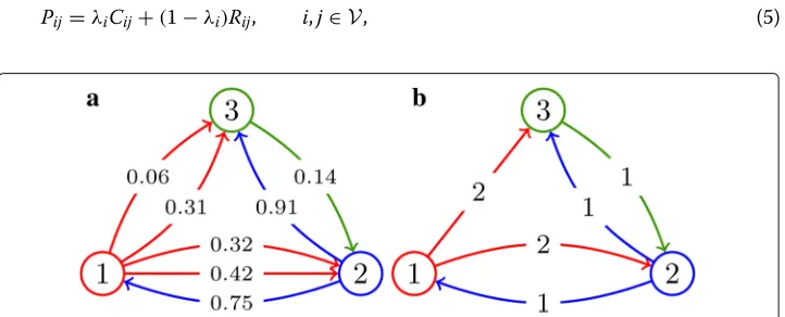
Figure1illustrates an example of the construction of an integrated network from link observations over a given time-window of durationT =1. In this example, the weighted adjacency matrix is equal to

W =

⎡ ⎢ ⎣

0 2 2 1 0 1 0 1 0

⎤ ⎥

⎦. (4)

Routing matrixP

The routing matrixPis constructed to encapsulate the information oni)the organization of nodes in nontrivial, hierarchical and overlapping communities;ii)the heterogeneous involvement of nodes in their communities, characterized through the presence of sources and drains; andiii)the existence of an irreducible backbone.

In order to distinguish the contribute of the community structure from that of the back-bone to the link generation process, we define matrixPas a convex combination of two n×nstochastic matricesCandR. The convex combination is weighted by an-dimensional nonnegative (entry-wise) vectorλ∈[ 0, 1]n, as

Pij=λiCij+(1−λi)Rij, i,j∈V, (5)

Fig. 1Exemplification of the construction of an integrated network in a time-window of durationT=1. In

(a), occurrences of links are plotted separately, along with their time-stamps (2 decimal digits). In (b), the integrated networkGTis illustrated. Weights represent the number of occurrences of each link in the

where matrixC, namedcommunity matrix, encodes the information on the role of the community-based mechanism in the link generation process, while matrixRencodes the role of the backbone in the process and is calledbackbone matrix. Toward a compact for-malization of the model, the community-free mechanism is considered as a special case of the community-based mechanism, through the inclusion into matrixCof the special all-to-all community, as detailed in “Community matrixC” section. In the following, unless specified differently, the termcommunity-basedwill refer to both the community-based and the community-free mechanisms, thus leaving aside only the backbone mechanism. Specifically, entryCijis the probability that nodeiconnects tojas a consequence of the community structure (including the all-to-all community), while entryRij is the prob-ability that such a connection is generated as a consequence of a dyadic relationship (backbone) betweeniandj. The entryλiweights the two mechanisms by quantifying the strength of the community-based mechanism in the process of link formation from node i. In general, the entries of vectorλare nonuniform, to capture the heterogeneous influ-ence of the two mechanisms for different nodes. The limit caseλi = 0 represents the scenario in which the community structure has no influence on the link generation pro-cess from nodeiand all its links are caused by the presence of the irreducible backbone, while the caseλi =1 models the case in which nodeiwires its connections only driven by the community structure.

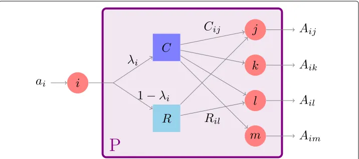
The mechanism governed by the convex combination in (5), illustrated in Fig.2, has an immediate probabilistic interpretation. When nodeiactivates, connections are driven by the community structure with probability λi, whereas they are driven by the back-bone mechanism with probability 1−λi. In the following, we will detail the construction principles of matricesCandR.

Community matrix C

Here, matrixCis designed to model a time-invariant community structure. This simpli-fying assumption is reflected in many real-world systems, where the pace of evolution of the community structure is much slower than the link generation process, as in (Bao and

Fig. 2Schematic of the mechanism governing a rADN model. Nodei∈Vactivates with rateai. Then, with

probabilityλiit generates a connection due the community-based mechanism, i.e., following the

probabilities in the community matrixC. Otherwise, with probability 1−λi, the link is caused by the

Michailidis2018). Different scenarios, where the community structure evolves in time, can be found in Rossetti and Cazabet (2018).

Given a time-invariant set ofk≥0 nontrivial communities, we label them with positive integer numbersh ∈ {1,. . .,k}. Trivial communities are the empty set, singletons, and the whole node setV. To model the community-free mechanism, we add anall-to-all trivial community that coincides with the whole systemV, labeled by index 0. Hence, the community set K = {0,. . .,k} comprises the trivialall-to-all community 0 and k nontrivial communities. Considering thehth community, we denote byVh⊆Vthe set of nodes that belong to it, whilenh:= |Vh|is its cardinality. On the other hand, considering the generic nodei∈V, we denote byCi:= {h:i∈Vh}the set of communities to which nodeibelongs, and withci:= |Ci|its cardinality.

We observe that the rADN paradigm allows each network node to belong to an arbitrary number of communities. This encompasses and generalizes the paradigm of modular ADNs (Nadini et al.2018b), where each node belongs to exactly one nontrivial commu-nity. The heterogeneous attitude of nodes in their different communities (Palla et al.2007) is modeled by defining a stochastic rectangular matrixQ∈[ 0, 1]n×(k+1), named commu-nity strength matrix, such thatQih>0 if and only ifi∈Vh. The entryQihis the probability that a link from nodeithat is caused by a community-based mechanism is wired within thehth community. The entries of matrixQcan be thus interpreted as the importance that each node gives to the each of the communities it belongs to. IfQihis large, nodeiacts as a source in communityh, generating many inter-community links. On the other hand, ifQihis small, then nodeiwill act as a drain, mostly receiving connections from other members. In this perspective, matrixQquantifies the strength of theactive involvement of nodes in each of their communities.

Formally, we define the community matrixC, entry-wise, as

Cij= ⎧ ⎨ ⎩

0 ifi=j

h∈Cj

Q_ihnh−1₁ otherwise. (6)

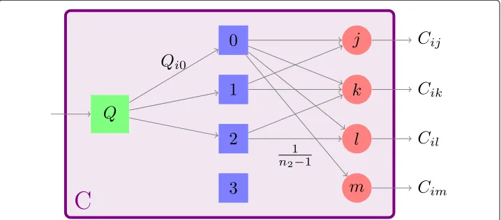
Figure3illustrates the mechanisms that govern the formation of the community matrix C. Specifically, when node i generates a connection following the community-based

Fig. 3Schematic of the mechanism that governs the community matrixC. First, a community is selected,

mechanism, first, it randomly selects a communityh ∈ Kto which it belongs, accord-ing to the probabilities in theith row of matrixQ. Then, it connects to a nodejchosen uniformly at random among thenh−1 nodes of thehth community (excluding nodei).

Backbone matrix R

Similar to the community structure, also the irreducible backbone is typi-cally fixed in time or it evolves much slower than the link formation process (Onnela et al. 2007; Gemmetto et al. 2017). Hence, here we hypothesize that this is constant for time-windows of reasonable duration.

The backbone is thus modeled by a time-invariant graphGR=(V,ER)and by a stochas-tic matrixR∈[ 0, 1]n×n, such thatRij>0 if and only if(i,j)∈ER. The entryRijmeasures the strength of the dyadic relationship between nodeiand nodejin a probabilistic frame-work. In many real-world scenarios of social and biological systems, it is reasonable to assume matrixRto be sparse, as observed from many empirical data sources (Newman 2003; Ballerini et al.2008).

We remark that, in the limit case where nodeiis not influenced by the backbone mech-anism, i.e.,λi=1, the entries of theith row of the backbone matrixRhave no influence on the link formation mechanism. Without any loss in generality, in this case we set the cor-responding rows of matrixRequal to the corresponding rows of an×nidentity matrix, i.e., we setRii=1 andRij=0, for anyj=i.

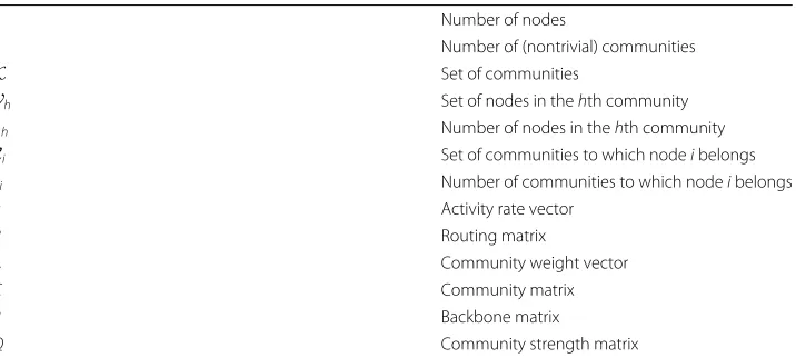
The set of parameters that characterize a rADN is summarized in Table1. To recapitu-late, taking into account the construction mechanism of matrixP, we detail the algorithm that summarizes the evolution of a rADN as follows:

1 att=0, the link set is set as empty (E(0)= ∅) and a Poisson clock (Bailey1990) with rateai(each one independent of the others) is initialized for each nodei∈V; 2 if at timet the clock associated with node i clicks, then node i activates and

randomly chooses whether the connection is generateda)by the community-based mechanism (with probabilityλi), or b) by the backbone (with probability1−λi). Then, depending on the previous choice, eithera)orb)occurs, where

a) nodei randomly selects a communityh∈K. Specifically, communityh is selected with probabilityQih. Then, nodej is chosen uniformly at random among thenh−1nodes of theh th community excluding node i ; or

Table 1Parameters that characterize a rADN model

n Number of nodes

k Number of (nontrivial) communities

K Set of communities

Vh Set of nodes in thehth community

nh Number of nodes in thehth community

Ci Set of communities to which nodeibelongs

ci Number of communities to which nodeibelongs

a Activity rate vector

P Routing matrix

λ Community weight vector

C Community matrix

R Backbone matrix

b) nodei randomly selects a nodej∈V. Specifically, nodej is selected with probabilityRij;

3 the directed link(i,j)is instantaneously added to the link setE(t); and

4 link(i,j)is immediately removed from the link set, the Poisson clock associated with nodei is re-initialized, and the algorithm is resumed to item 2.

We observe that our extended rADN modeling framework actually encompasses many variants of standard ADNs proposed in the recent literature. Some relevant examples are presented in the following.

Standard ADNs

Standard continuous-time ADNs (Zino et al.2016) are obtained by settingλi=1,i∈V, andK= {0}. This choice yieldsPii =0, for anyi∈V, and

Pij=Cij=

Qi0 n−1 =

1

n−1, i∈V,j∈V{i}. (7)

Modular ADNs

Modular ADNs (Nadini et al.2018b) can be derived as a particular case of rADN with λi=1,∀i∈V. Here, the set of communitiesKdefines a partition of the node set where each node belongs to one and only one community. The notation used in the original incarnation defined in Nadini et al. (2018b) can be retrieved by settingQi0=1−μ,Qih= μ,∀i∈Vh. In this case, (6) readsPii =0,∀i∈V, and, for anyj=i,

Pij=Cij= ⎧ ⎨ ⎩

1−μ

n−1+nh−μ1 ifi∈Vh,j∈Vh, 1−μ

n−1 ifi∈Vh,j∈/Vh.

(8)

ADNs with attractiveness

Attractiveness has been added to ADNs to model the heterogeneous propensity of nodes to receive connections (Pozzana et al.2017; Alessandretti et al.2017). Specifically, given an attractivity vectorb > 0 (entry-wise), the probability that a node generates a link to nodej∈Vis proportional tobj. In the framework of rADNs, this feature can be modeled by settingλi=0,∀i∈V, and all the entries of the backbone matrixRas

Rij=

bj k∈V{i}bk

, ∀i,j∈V. (9)

Estimation of the model parameters from empirical data

Here, we develop a technique to identify the model parameters. Specifically, we estimate the activity rate vectora, the weight vectorλ, the community strength matrixQ, and the backbone matrixR. The objective of the technique presented in this section is to devise a procedure to deepen the characterization of communities, shading light on the diverse role of their members and their role in the link formation process.

Parameter identification procedure

W; andii)the community setKand the setsVh,h ∈ K, obtained as the output of the community detection algorithm. According to (Perra et al.2012), the activity rate vector can be estimated as

ˆ ai=

j∈V

Wij

T , i∈V. (10)

The expected number of occurrences of the link(i,j), denoted by W¯ij, is computed following (3), and it is equal to

¯

Wij= ˆaiT

h∈Ci λiQih

1 nh−1 + ˆ

aiT(1−λi)Rij. (11)

In order to estimate the other model parameters, i.e., the community weight vectorλ, the community strength matrixQ, and the backbone matrixR, we formulate the identi-fication problem in terms of a constrained optimization program. We observe that the identification problem is naturally underdetermined. In fact, the observed data consists of an×nmatrix, while the set of parameters to be estimated comprises an×nmatrix, an×(k +1) matrix, and an-dimensional vector. Hence, except for unlikely particu-lar cases, the number of parameters to be estimated exceeds the number of equations that can be written using the available data. To address this issue, we introduce a free parameter vectorγ ∈[ 0, 1]n, namedcommunity belief, which measures our belief in the prominence of the role of the community-based mechanism in the link formation process. Tuning this parameter vector is the most delicate task in the application of our method. In “Confidence interval for the community belief parameter” section, we put forward a sta-tistical procedure to assess a confidence interval for such a parameter vector. In particular, we identify the largest value forγ that is compatible with the observed data, which yields the characterization of the system with the highest belief in the community-based link formation mechanism. Such a model is often preferred, as it leads to a characterization at a mesoscopic level, whereby the system characteristics are captured with a good detail and an intermediate granularity, which ensures a good description of the system behavior without incurring in the issues related to a microscopic, node-based representation. How-ever, in “Validation on synthetic networks” section we show that when the dataset has a small size, smaller values of the parameterγ within the prescribed confidence interval may be more suitable to describe the system without overfitting the community structure. The identification problem is formalized by writing a set ofndisjoint minimization problems, one for each nodei∈V. Specifically, for nodei∈V, we want to minimize the function

f(εi•,Qi•,Ri•,λi)=(1−γi) n

j=1 ε2

ij+γi(1−λi)Rij, (12)

with respect to variableλiand the entries of theith row of matricesε,QandR, written in compact form asεi•,Qi•, andRi•, respectively. The minimization problem in (12) is subject to several constraints: we require that the number of occurrences of the link(i,j), i.e.,Wij, is equal to its expected valueW¯ij, computed according to (11), up to some natural statistical fluctuation, modeled by the residual εij; we also require the matricesQand

⎧ ⎪ ⎪ ⎪ ⎪ ⎪ ⎪ ⎪ ⎪ ⎪ ⎪ ⎪ ⎪ ⎪ ⎨ ⎪ ⎪ ⎪ ⎪ ⎪ ⎪ ⎪ ⎪ ⎪ ⎪ ⎪ ⎪ ⎪ ⎩ ˆ aiT

h∈Ci

λiQihnh−11+ ˆaiT(1−λi)Rij+εij=Wij ∀j∈ {1,. . .,n},

h∈Ci

Qih=1,

n j=1

Rij=1,

0≤Qih≤1, ∀h∈Ci,

0≤Rij≤1, ∀j∈ {1,. . .,n},

0≤λi≤1.

(13)

We observe that the objective function in (12) consists of the sum of two terms: the first summand is the sum of the squared residuals, whose minimization allows for obtaining a model that is compatible with the observed data; the second summand is a cost related to the contributions of the backbone-based mechanism. In the absence of the second term, a trivial solution would beλi=0 andRij= ¯Wij/aˆi, that is, the whole link formation process is explained in terms of dyadic relationships between nodes. However, this is often not consistent with the empirical observation of a sparse backbone in systems of different nature (Ballerini et al.2008; Newman2003), and it fails to provide a description of the system at a mesoscopic scale.

Although the constraints are nonlinear, the change of variable

˜

Qih:=λiQih R˜ij:=(1−λi)Rij, (14)

allows us to write (12) as a quadratic programming problem (Boyd and Vandenberghe 2004) with linear constraints, which can be solved with a reasonable computational effort. Specifically, the objective function reads

f

εi•,Q˜i•,R˜i•,λi

=(1−γi) n

j=1 ε2

ij+γiR˜ij, (15)

subject to the following constraints: ⎧ ⎪ ⎪ ⎪ ⎪ ⎪ ⎪ ⎪ ⎨ ⎪ ⎪ ⎪ ⎪ ⎪ ⎪ ⎪ ⎩ ˆ aiT

h∈Ci ˜

Qihnh−11+ ˆaiTR˜ij+εij=Wij ∀j∈ {1,. . .,n},

h∈Ci

˜ Qih+

n j=1 ˜ Rij=1,

0≤ ˜Qih≤1, ∀h∈Ci,

0≤ ˜Rij≤1, ∀j∈ {1,. . .,n}.

(16)

The computational complexity of the parameter identification method proposed here can be estimated as a function of the numbernof nodes inV, the numbermof nonzero entries of the weighted adjacency matrixW, and the numberkof communities. Specifi-cally, we obtain that the computational complexity is equal toOn2+nm+nk. Since it often holdsk<<n, we conclude that, for sparse integrated networks the computational complexity isOn2, while for dense networks it isOn3.

Confidence interval for the community belief parameter

whole link formation process from nodeiis explained in terms of the backbone. Then, when γi grows, the role of communities in the process of link generation gains more importance. Whenγiis too large, however, the role of communities in the link formation process might be overestimated and the models obtained for these values of the com-munity belief parameter are not statistically compatible with the data observed. Here, we put forward a technique to identify the largest value of the community beliefγisuch that the parameters of the rADN model identified for that value ofγiare compatible with the available data.

Fixing a value of the parameterγi, the minimization problem (15) can be solved by means of a quadratic programming solver. We denote the corresponding solution asQ(γi)_, R(γi)_{, and}λ(γi)_{. Using the parameters estimated with this solution, and the expression for} the probability of link formation in rADN in (3), we can determine the distribution of the ith row of the weighted adjacency matrixW. We denote such a row asW(γi)

i• , to stress its dependence on the choice of the parameterγi. Specifically, each row entryW_ij(γi)is a Poisson random variable, independent of the others, with expected value

¯ W(γi)

ij =λ (γi) i

h∈Ci Q(γi)

ih

nh−1+

1−λ(γi) i

R(γi)

ij . (17)

Hence, the likelihood that theith row of the observed weighted adjacency matrixWis a realization of the random variableW(γi)_{is given by}

LW¯(γi)|_W= n

j=1

¯ W(γi)

ij Wij

e− ¯W

(γi) ij

Wij!

, (18)

which is the probability that the realization of thenindependent Poisson distributed ran-dom variables with expected values computed according to (17) coincide with theith row of the observed matrixW. Since the product of small probabilities is numerically unstable, it is convenient to test the log-likelihood (Boyd and Vandenberghe2004) instead of (18), which is

logLW¯(γi)|_W= n

j=1 log ⎛ ⎜ ⎝ ¯ W(γi)

ij Wij

e− ¯W

(γi) ij

Wij!

⎞ ⎟

⎠. (19)

adjacency matrixW. To this aim, we perform a Likelihood Ratio (LR) test (Casella and Berger2002). The LR test determines whether the null hypothesis that the observedith row of the weighted adjacency matrixWi•is obtained from a vector of independent Pois-son variables with expected valuesW¯(γi)

ij from (17), forj= 1,. . .,n, should be rejected. Specifically, fixing a significance coverageα∈[ 0, 1], the LR test rejects the null hypothesis if the statistic

D:=2

logL

¯ W(0)|W

−logL

¯

W(γi)|_{W (20)}

is greater than a threshold q1−α, where q1−α is the(1−α)-quantile of a chi-squared distribution withn−1 degrees of freedom (Casella and Berger2002). We remark that the reduction of the degrees of freedom of the distribution fromnton−1 is due to the absence of self-loops.

It is worth noticing that the statisticDis a monotonic increasing function ofγi. Hence, fixing a significance coverageα ∈[ 0, 1], the LR test ultimately identifies a thresholdγ¯i, equal to the value for which the statisticDis equal to the(1−α)-quantile of a chi-squared distribution withn−1 degrees of freedom. All the values ofγi >γ¯iare rejected. Hence, our procedure establishes a confidence interval for the parameterγi of the form γi ∈ [ 0,γ¯i]. Unfortunately, the valueγ¯i that produces the significance coverageα cannot be derived analytically. However, since the statisticDis monotone inγi, several numerical methods can efficiently retrieve a good approximation of the thresholdγ¯i (Hammings 1973).

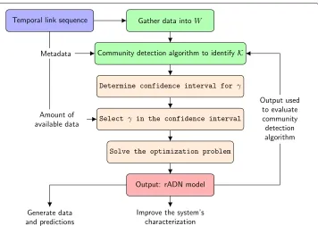
The technique described above identifies a range for theith componentγiof the com-munity belief vector γ that is compatible with the empirical data. Implementing this procedure for all the nodesi∈ V, we obtain a confidence interval for the whole param-eter vectorγ, which is then-dimensional hyperrectangleγ ∈[ 0,γ¯1]× · · · ×[ 0,γ¯n]. This yields a set of mathematical models that are compatible with the observed data. The parameter vector may be tuned within this hyperrectangle, depending on the user’s belief in the community structure, on the amount of data available (as we will discuss in “Validation on synthetic networks” section) and, possibly, on additional information avail-able on the systems such as historical data, or measurements on similar systems. We refer to the model obtained withγi = ¯γi, for alli∈V, as the model with the largest belief in the community structure, among those compatible with the observed data. The flow chart in Fig.4summarizes the whole procedure of our parameter identification method, from the data consisting of a sequence of temporal links, to the definition of an rADN model.

Validation on synthetic networks

Fig. 4Flow chart of the parameter identification method. Data on the temporal connections are gathered into the weighted adjacency matrixWof the integrated network. Then, a community detection algorithm is used to preliminary detect a set of communities. The community detection algorithm may be enriched by available metadata. A confidence interval for the community belief is then computed and the parameter_γis selected within this interval, on the basis the available data. Finally, fixed_γ, the model parameters are identified through the solution of an optimization problem. A rADN model statistically compatible with the available data is eventually derived. The output of such a model can be used to assess and improve the performance of existing community detection algorithms or, on its own, to enrich the characterization of the system and to generate data and predictions that are compatible with the available data

characterized by overlapping communities, is discussed in “Overlapping communities” section. Also in these cases, we successfully perform the parameter identification by means of the method proposed in this work.

Exclusive heterogeneous communities

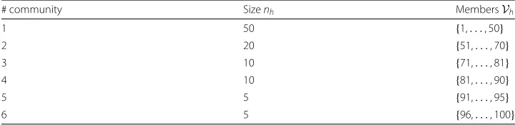
We generate a network with an exclusive community structure, where each node belongs to one and only one nontrivial community. We partitionn=100 nodes intok= 6 non-trivial communities with heterogeneous size, as shown in Table2. Thus, the community setKand the setsVh,h∈Kare known.

Table 2Benchmark with exclusive community structures

# community Sizenh MembersVh

1 50 {1,. . ., 50}

2 20 {51,. . ., 70}

3 10 _{71,_{. . .}, 81_}

4 10 {81,. . ., 90}

5 5 {91,. . ., 95}

6 5 {96,. . ., 100}

The backbone matrixRis defined as follows. First, we construct the graphGR=(V,ER), corresponding to the backbone, according to an Erdös-Rényi random graph model (Erd˝os and Rényi1959) with parameterp = 4/99. Such a choice of the parameterpproduces a network with average degree equal to 4. Specifically, link(i,j) ∈ ERwith probabilityp, each link independently of the others. Then, the entriesRij, for(i,j) ∈ ER, are assigned uniformly at random, such that each row sums 1, while all the other entries of the row are set to 0. In the extreme case in which nodei∈ Vhas no outgoing links, then we set the diagonal entryRii = 1, all other entries equal to 0, and the corresponding λi = 1. The other entries of the vectorλ(i.e., those corresponding to nodesithat have at least an outgoing link in the backbone) are realizations of independent beta-distributed random variables with mean 0.71 and variance 0.01. Finally, the activity potentials are selected as realizations of independent and identically power-law distributed random variables with exponent equal to−2.5 and lower cut-offamin=0.01. The resulting routing matrixPis represented through a color-coded graph in Fig.5b.

The system is then simulated for a time-window of durationT and the data corres-ponding to the integrated network are stored in the weighted adjacency matrixW.

Initially, we test the capability of our technique to correctly identify the model parame-ters when a sufficiently large amount of data is available. Then, we study the performance of our method in a critical scenario in which the system is observed for a short time-window and the data vector of temporal links is much smaller, in order to appreciate the effectiveness of the approach even in this situation.

In our first analysis, we set T = 106 and we observe approximately 1,500,000 temporal connections during the time-window. We apply our parame-ter identification technique by setting the community belief parameparame-ter γi equal

Fig. 5Matrices characterizing the benchmark with exclusive communities. In (a), the community strength

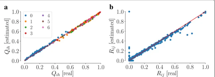
to the maximum value of the confidence interval identified through the pro-cedure proposed in “Confidence interval for the community belief parameter” section, i.e.,γi= ¯γi,∀i∈V. This choice is the one that allows us to explain the largest part of the link generation process in terms of communities, compatibly with the observed data. Figure6illustrates the accuracy of our method in the estimation of matrixQ. We observe that the nonzero entries of matrixQare estimated with a high accuracy, and without any bias related to the size of the communities and the heterogeneity in the parameters. In fact, accuracy does not change over the different communities, associated with different colors in Fig.6, and it is high both for small and for large values ofQijand

Rij. Specifically, the mean square error of the estimated entries of matrixQvaries from 0.011 to 0.020 over the communities, with no statistically significant difference between them, while for the entries of matrixR, it is equal to 0.012. In additional simulations, here omitted for brevity, we have observed that increasing the number of communitieskhas no significant effect on the performance of our parameter identification method.

In our second analysis, we reduce the size of the data vector, settingT = 105and T = 104, and generating approximately 150,000 and 15,000 temporal connections, respectively. Figure 7 reveals that, when the system can be observed only for a short time-window and few temporal links are observed, the choice of the largest value of the community belief γi in its confidence interval may lead to an overestimation of the contribution of the communities in the link generation process. We observe from Fig. 7a-b that the entries of vector λ, which weight the contribution of communi-ties in the link generation mechanism, tend to be overestimated for small values of T. In fact, the mean square error of the estimated entries of vector λ increases from 0.020 for T = 106, to 0.055 and 0.185, for T = 105 and T = 104, respectively. We believe that the overestimation of the community weights is a com-mon phenomenon when the number of temporal links is small. To address this issue, we suggest to reduce the value of the parameter γi, within the confidence interval established in “Confidence interval for the community belief parameter” section. Figure8shows that, also with few data available, an accurate estimation of the vector λand a good estimation of the community strength matrixQcan be obtained by selecting smaller values for the community belief parameter vector. In Fig.8a we can appreciate an excellent agreement between the estimated community weight vector and

Fig. 6Validation on the synthetic benchmark with exclusive communities. Estimation of the nonzero entries

of (a) the community matrixQand (b) the backbone matrixRfor the benchmark with exclusive communities, from data sampled over a time-window of durationT₌106_{. The parameters are set asγ}

i= ¯γi,∀i∈V.

Fig. 7Dependence of the identification performance on the duration of the time-windowT. Estimation of the entries of the weights vectorλfor increasing duration of the time-windowT, withγi= ¯γi,∀i∈V. For

small values ofT, settingγi= ¯γiseems to yield an overestimation of the contribution of communities in the

link generation mechanism

the actual one (mean square error equal to 0.003). In Fig.8b we observe that, even though the accuracy in the estimation of the matrixQis reduced with respect to the case with largeT, there is still a satisfactory agreement between the estimated entries of the com-munity strength matrix and the corresponding real quantities (mean square error equal to 0.091). In our simulations, we select the value for the community belief parameter vec-torγ by performing a bisection method in the rangeγi ∈[ 0,γ¯i], to minimize the absolute deviation between the estimated vectorλand the original benchmark community weight vector. This confirms our intuition that the best model estimation is within the confi-dence interval we have assessed. In our example, we observe that, when the temporal link set is reduced to the 1% of the original amount (i.e., 15,000 links), the optimal value for gamma is found to be in average the 18% of the extreme valueγ¯. In real-world scenarios, where the real values ofλare unknown, the optimal selection of parameterγ remains an open problem, which will be tackled in our future research.

Hierarchical communities

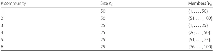
Here, we assess our method on a second benchmark in which communities present a hierarchical structure. Specifically, we define a two-level hierarchy: nodes are first parti-tioned into two first-level communities, then, each of these communities is split into two second-level communities. Each node thus belongs to a first-level community and to a second-level one, besides the all-to-all community. Details are reported in Table3.

Fig. 8Identification performance forTsmall, reducingγi. Estimation of (a) the vectorλand (b) the matrixQ

forT=104_{, using the optimal value ofγ}

i∈[ 0,γ¯i],i∈V, selected using a bisection method. The optimal

Table 3Benchmark with hierarchical community structures

# community Sizenh MembersVh

1 50 {1,. . ., 50}

2 50 {51,. . ., 100}

3 25 _{1,_{. . .}, 25_}

4 25 {26,. . ., 50}

5 25 {51,. . ., 75}

6 25 {76,. . ., 100}

Matrix Q is generated similarly to the previous benchmark. The entries of its first column are selected from a beta distribution with mean 0.25 and variance 0.02, each one independent of the others. The other two nonzero terms of each row are real-izations of uniformly distributed random variables, normalized to obtain a stochastic matrix. Matrix Q obtained according to this procedure is illustrated, through color coding, in Fig. 9a. Then, the backbone matrixR, the weight vector λ, and the activ-ity rate vectoraare generated following the same procedure described in the previous section.

The system is simulated for a time-window of durationT = 106, obtaining approx-imately 1,500,000 temporal connections, the weighted adjacency matrixW of the inte-grated network is generated, and our technique is used to estimate the parameters. The results of our analysis, illustrated in Fig.7b-c, suggest that our method is also able to deal with hierarchical community structures. We observe that we are able to identify the model parameters with a high accuracy and without any bias due to the different levels in the hierarchical community structure. In fact, in Fig.9c, we observe that there is no sig-nificant difference in the accuracy of the estimation of the entries corresponding to the first-level communities (i.e., 1 and 2) and the second-level ones (i.e., 3–6). Specifically, the mean square error of the estimated entries of matrixQvaries over the communities from 0.015 to 0.025 (in average, it is equal to 0.021 for the first-level communities and 0.017 for the second-level ones, with no statistically significant difference between the two quantities). Finally, we observe that, also in this case where hierarchical communities are present, the problem of a reduced size of the data vector can be addressed by reducing the tradeoff parameter vectorγ, in order to avoid data overfitting. Results are omitted for brevity.

Overlapping communities

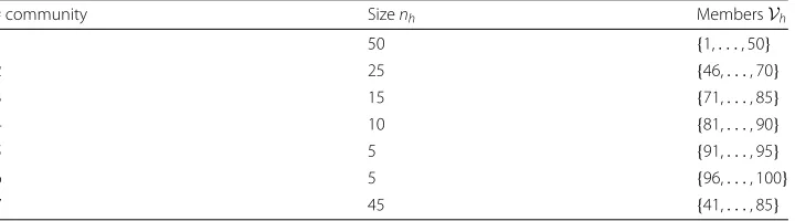
Finally, we consider a benchmark in which communities have an overlapping structure. Then=100 nodes are divided into 7 communities, as detailed in Table4.

The community structure presents several overlaps, notably between communities 2,3,4, and 7. The community strength matrixQ(illustrated in Fig. 10a), the backbone matrixR, as well as the two vectorsλandaare defined following the procedure presented in the previous benchmarks. Then, the system is simulated for a time-window of duration T =106, generating approximately 1,500,000 temporal connections, and our technique is used to identify the parameters from the weighted adjacency matrixW of the integrated network obtained from our simulations. Also in this scenario, as illustrated in Fig.10b and c, our method is able to identify the model parameters with high accuracy and is free of any bias due to the presence of overlaps between the communities. In fact, in Fig.10b we observe that the accuracy in the estimation of the entries of the community weight vectorλare not influenced on whether a node belongs to an overlapping community or not: the average mean square error for the nodes in overlapping communities is equal to 0.019, while for nodes not in overlapping communities is equal to 0.015, with no statisti-cally significant difference between the two quantities. Similarly, also the outcome of the estimation of the community strength matrixQis not influenced by the presence of over-laps between the communities, as can be observed in Fig.10c, by comparing nodes that belong to different communities. In fact, the mean square error of the estimated entries of matrixQvaries over the communities from 0.013 to 0.023 (in average, it is equal to 0.015 for the communities with no overlaps and 0.017 for the overlapping ones, with no statis-tically significant difference between the two quantities). Also in this case, the tradeoff parameter vectorγ can be set to a smaller value than the extremeγ¯to avoid overestima-tion ofλwhen little data is available, similarly to what discussed in the case of exclusive communities.

Case studies Enron email corpus

We use our method to enrich the results of community detection for a real-world case study: the Enron email corpus (Cohen). This is a dataset of more than 500,000 emails sent by the 158 employees of Enron company from 1979-12-31 to 2002-06-21, when the company failed. In order to deal with a uniform dataset, in which the community structure and the irreducible backbone can be assumed to be constant, we restrict the dataset to the portion of mails sent after 1998-11-13. We also remove self-sent emails and nodes that do not send or receive any email. After such a data cleaning procedure, we obtain a dataset

Table 4Benchmark with overlapping community structures

# community Sizenh MembersVh

1 50 _{1,_{. . .}, 50_}

2 25 _{46,_{. . .}, 70_}

3 15 {71,. . ., 85}

4 10 {81,. . ., 90}

5 5 {91,. . ., 95}

6 5 _{96,_{. . .}, 100_}

Fig. 10 Validation on a synthetic network with overlapping communities. In (a), matrixQis illustrated (color intensity is proportional to the value of the entry). Estimations of the vectorλand of the matrixQare shown in (b) and (c), respectively. Different colors in (c) indicate different communities

withn = 143 employees and 108,786 emails, which identify a temporal network where each employee is a node and each email determines a link from the sender to the receiver. We then use a community detection algorithm on the integrated network to identify the community structure. We observe that the application of different algorithms for com-munity detection may lead to the identification of different comcom-munity structures. As stated in the introduction, our method can be used to establish a criterion to discrim-inate among the outcome of different community detection algorithms. In fact, for any community structure obtained by means of a different community detection algorithm, we can identify the model parameters using our method, and then compare the average entry of the community weight vectorλover the nodes, namely

< λ >:= 1 n

i∈V

λi. (21)

This quantity measures the fraction of links that can be statistically explained by means of a community-based mechanism. Therefore, the community structure that is able to produce the highest value of< λ >is the one that is able to explain the largest part of the link formation process.

In our case study, we apply three different algorithms to detect the communities from the integrated network: Infomap (Rosvall and Bergstrom2008), Louvain (Blondel et al. 2008), and OSLOM (Lancichinetti et al.2011). Since the community detection algorithms are based on randomized techniques, we perform 100 runs of each algorithm. For each of these 300 outputs, we perform our parameter identification method. The community belief vectorγ is chosen within its confidence interval by using a bisection method to maximize the value of< λ >. Then, for each of the three community detection algo-rithms, we select the run that yields the largest value of< λ >. The estimated matrices Qfor the three different algorithms are illustrated and compared in Fig.11. We observe that the three outputs are significantly dissimilar, since a different number of communi-ties is originally detected. Specifically, we observe that the largest community identified by Louvain is split into two or more small communities by the other algorithms. Despite these differences, we can identify some common patterns. For instance, there is a first group of 17 nodes that belong to a “strong” community, where members have high ten-dency of generating inter-community links. This feature of the system emerges from all of the three outputs, as can be observed by comparing the different panels of Fig.11.

Fig. 11 Results of our parameter identification method on the Enron email corpus case study. MatrixQis estimated, starting from the community structure detected by using (a) Infomap, (b) Louvain, and (c) OSLOM

in fact, in each of the runs it always retrieves the same community partition. Louvain, instead, identifies 6 different outcomes in the 100 runs, whereas OSLOM produces a different outcome in each run. In Fig.12a, we plot the overlapping normalized mutual information (ONMI) evaluated between each pair of partitions produced by the same method (McDaid et al.2011). This figure supports our claim that the output of OSLOM is strongly unstable, since each run produces a different outcome. In fact, the correla-tion between two different outputs can be small, as seen in the box-plot. Instead, the six different outputs of Louvain algorithm are strongly correlated. In Fig.12b, the distribu-tion of the value of< λ >in different runs of the algorithm is illustrated. We observe that Infomap outperforms the other two algorithms, while OSLOM and Louvain seem to have a similar performance. Finally, in Fig.12c we plot the ONMI of an OSLOM partition with the Infomap partition as a function of the quantity< λ >. From this figure, we can observe a significant positive correlation between the two quantities, which supports our intuition that< λ >might be used as a performance index of the community detection algorithm.

Primary school

We apply our algorithm to a second real-world case study: the SocioPattern primary school dataset (SocioPatterns). This dataset consists of a temporal network of face-to-face interactions between students and teachers in a French primary school, recorded via proximity sensors. The dataset comprises 77,602 interactions (sampled with a time reso-lution of 20s) betweenn=242 individuals over a time-window of durationT =2 days.

Fig. 12 Comparison between different community detection algorithms for the Enron email corpus case

In this dataset, individuals are naturally partitioned: 232 of them are students, divided into 10 classes, and 10 are teachers (Stehlé et al.2011; Gemmetto et al.2014). These metadata provide a ground truth for the community structure. The main limitation of this dataset is that the direction of the interactions is not known, since it cannot be registered by the proximity sensors. In order to apply our method, in the absence of exact information on the link direction, we assume it to be homogeneously distributed. Hence, we perform a Monte Carlo parameter identification over 100 runs in which we randomize over the direction of each link in the dataset. Specifically, for each undirected link{i,j}, we inter-pret it as a directed link fromitojwith probability 1/2, and as a directed link fromjtoi, otherwise, each one independent of the others. Since classes provide an evidence on the ground truth of the community structure and the number of interactions in the dataset is sufficiently large, we set the largest value of belief parameter within its confidence inter-val, i.e.,γi = ¯γi, for alli ∈ V. Then, we evaluate the average vectorλˆ and the average matricesQˆ andRˆover the multiple realizations.

The results illustrated in Fig.13show that our model is able to capture the community structure of the system, supporting the hypothesis that comes from the natural partition of students into their classes. In fact, the distribution ofλˆillustrated in Fig.13a shows that the class-based community structure is able to describe a large part of the observed links for most of the nodes. This can also be observed by the large involvement of members in their communities, illustrated in Fig.13b. Notably, the teachers, corresponding to the last row of Fig.13b, make an exception: they have small values ofQˆ within their community (last column), while they have a large involvement in the all-to-all community. This seems to reflect the reality, since a teacher often interacts more with students (of several classes) than with other teachers. It is worth noticing that this is an information that a traditional community detection algorithm can hardly reveal. In addition, a more detailed structure of dyadic relationships, both within and outside the classes, is revealed in the backbone matrixRˆ represented in Fig.13c. From its structure, one can infer the presence of strong relationships between students, mostly classmates. From these interactions one can infer the presence of subcommunities within each class and use this information to reconstruct a hierarchical community structure. It also worth noticing that, for last-years students (the last rows before teachers), the dyadic relationships in the backbone are not limited to

Fig. 13 Monte Carlo parameter identification (over 100 random link orientations) for the primary school case

the classmates, but also inter-classes nonzero entries are present. This is consistent with other analyses performed on the same dataset, which show that last-years students are more active in generating out-of-class relationships (Stehlé et al.2011; Gemmetto et al. 2014).

Conclusion

In this paper, we deal with the problem of modeling and characterizing the complex network structure of real-world systems. First, we present a mathematical model for tem-poral networks that generalizes the ADN paradigm, by including link directionality, the presence of a heterogeneous, hierarchical, and overlapping community structure, and the existence of an irreducible backbone of connections. Then, based on this model, we pro-pose a technique to estimate the model parameters from empirical data and assess the effect of communities and the irreducible backbone on the link generation process into an intelligible form, providing a mesoscopic description of the system at the communities level. The proposed technique is based on the introduction of a free parameter that can be calibrated within a confidence interval. This parameter models our belief in the role of communities in the link formation mechanism. We validate our method on three differ-ent synthetic networks and on a real-world case study, with satisfactory results. We also apply our method to two different real-world case studies. In the first one, the ground truth about the community structure is unknown and our method is used to establish a criterion to assess the performance of different community detection algorithms. In the second scenario, a ground truth about the community structure is instead provided by the partition of students and teachers in classes. In this case, we are able toi)retrieve the actual partition in classes andii)reveal the different role of students and teachers in their classes.

The presented method is characterized by a reasonable computational effort. This prop-erty, together with the possibility of analytical treatment exhibited by ADNs, is essential to tackle real-world problems. For example, the possibility to detect the role of nodes and communities in interactions between individuals allows for the design of accurate tar-geted immunization strategies for the case of disease spreading (Masuda2009; Salathè and Jones2010; Gong et al.2013), or for the detection of closed communities that drive the spread of misinformation and fake news, named echo chambers (Del Vicario et al. 2016). For these reasons, we believe that the possibility of unveiling the architecture of a complex system, through the characterization of its community structure, may play a fun-damental role in the development of effective techniques to address real-world problems, with potential invaluable benefits to the society.

Abbreviations

ADN: activity driven network; LR: likelihood ratio; ONMI: overlapping normalized mutual information; OSLOM: order statistics local optimization method; rADN: routed activity driven network

Acknowledgment

The authors acknowledge the SocioPatterns collaboration.

Funding

Availability of data and materials

The datasets generated during the current study are available upon request. The source code used to perform the parameter identification is avaialble athttps://github.com/cbongiorno/RADNFIT. The datasets analyzed in the case study is available in the Enron Email Dataset (https://www.cs.cmu.edu/~./enron/) and in the SocioPatterns Primary School Temporal Network Data (http://www.sociopatterns.org/datasets/primary-school-temporal-network-data/), respectively.

Authors’ contributions

AR coordinated the research; CB performed the numerical studies and conceived the parameter identification method; LZ designed the model and wrote the initial draft; all authors contributed to data analysis and writing the final manuscript. All authors read and approved the final manuscript.

Competing interests

The authors declare that they have no competing interests.

Publisher’s Note

Springer Nature remains neutral with regard to jurisdictional claims in published maps and institutional affiliations.

Author details

1_{Department of Electronics and Telecommunications, Politecnico di Torino, Corso Duca degli Abruzzi, 24, 10129 Torino,} Italy.2_{Department of Mathematical Sciences “G.L. Lagrange”, Politecnico di Torino, Corso Duca degli Abruzzi, 24, 10129} Torino, Italy.3_{Office of Innovation, New York University Tandon School of Engineering, 11201 Brooklyn NY, US.}

Received: 6 December 2018 Accepted: 6 March 2019

References

Alessandretti L, Sun K, Baronchelli A, Perra N (2017) Random walks on activity-driven networks with attractiveness. Phys Rev E 95(5):052318

Bailey NTJ (1990) The Elements of Stochastic Processes with Applications to the Natural Sciences. Wiley, New York Ballerini M, Cabibbo N, Candelier R, Cavagna A, Cisbani E, Giardina I, Lecomte V, Orlandi A, Parisi G, Procaccini A, Viale M,

Zdravkovic V (2008) Interaction ruling animal collective behavior depends on topological rather than metric distance: Evidence from a field study. Proc Natl Acad Sci USA 105(4):1232–1237

Bao W, Michailidis G (2018) Core community structure recovery and phase transition detection in temporally evolving networks. Sci Rep 8(1):12938

Benson AR, Gleich DF, Leskovec J (2016) Higher-order organization of complex networks. Science 353(6295):163–166 Bishop C (2006) Pattern Recognition and Machine Learning. Springer, New York

Blondel VD, Guillaume J-L, Lambiotte R, Lefebvre E (2008) Fast unfolding of communities in large networks. J Stat Mech Theory Exp 2008(10):10008

Bongiorno C, Zino L, Rizzo A (2018) On unveiling the community structure of temporal networks. In: Proceedings of the 57th IEEE Conference on Decision and Control (CDC). pp 6210–6215

Boyd S, Vandenberghe L (2004) Convex Optimization. Cambridge University Press, New York Casella G, Berger RL (2002) Statistical Inference, vol. 2. Duxbury, Pacific Grove

Cohen WW Enron Email Dataset.https://www.cs.cmu.edu/~./enron/. Accessed 27 Feb 2019

Del Vicario M, Bessi A, Zollo F, Petroni F, Scala A, Caldarelli G, Stanley HE, Quattrociocchi W (2016) The spreading of misinformation online. Proc Natl Acad Sci USA 113(3):554–559

Erd ˝os P, Rényi A (1959) On random graphs. Publ Math Debrecen 6:290–297

Estrada E (2011) The Structure of Complex Networks: Theory and Applications. Oxford University Press, Oxford Fortunato S, Hric D (2016) Community detection in networks: A user guide. Phys Rep 659:1–44. Community detection in

networks: A user guide

Gemmetto V, Cardillo A, Garlaschelli D (2017) Irreducible network backbones: unbiased graph filtering via maximum entropy. arXiv preprint arXiv:1706.00230

Gemmetto V, Barrat A, Cattuto C (2014) Mitigation of infectious disease at school: targeted class closure vs school closure,. BMC Infect Dis 14(1):695

Girvan M, Newman MEJ (2002) Community structure in social and biological networks. Proc Natl Acad Sci USA 99(12):7821–7826

Gong K, Tang M, Hui PM, Zhang HF, Younghae D, Lai Y-C (2013) An efficient immunization strategy for community networks. PLoS ONE 8(12):1–11

Hammings R (1973) Numerical Methods for Scientists and Engineers, 2nd edition. Dover Publications, New York Holme P, Saramäki J (2012) Temporal networks. Phys Rep 519(3):97–125

Karsai M, Perra N, Vespignani A (2014) Time varying networks and the weakness of strong ties. Sci Rep 4:4001 Khan BS, Niazi MA (2017) Network community detection: A review and visual survey. arXiv preprint arXiv:1708.00977 Lancichinetti A, Fortunato S, Kertész J (2009) Detecting the overlapping and hierarchical community structure in complex

networks. New J Phys 11(3):033015

Lancichinetti A, Radicchi F, Ramasco JJ, Fortunato S (2011) Finding statistically significant communities in networks. PLoS ONE 6(4):1–18

Latapy M, Viard T, Magnien C (2018) Stream graphs and link streams for the modeling of interactions over time. Soc Netw Anal Min 8(1):61

Lei Y, Jiang X, Guo Q, Ma Y, Li M, Zheng Z (2016) Contagion processes on the static and activity-driven coupling networks. Phys Rev E 93(3):032308