A learned sparseness and IGMRF-based regularization framework for dense disparity estimation using unsupervised feature learning

(1)

R E S E A R C H P A P E R

Open Access

A learned sparseness and IGMRF-based

regularization framework for dense disparity

estimation using unsupervised feature

learning

Sonam Nahar

1*

and Manjunath V. Joshi

2

Abstract

In this work, we propose a new approach for dense disparity estimation in a global energy minimization framework. We propose to use a feature matching cost which is defined using the learned hierarchical features of given left and right stereo images and we combine it with the pixel-based intensity matching cost in our energy function. Hierarchical features are learned using thedeep deconvolutional networkwhich is trained in an unsupervised way using a database consisting of large number of stereo images. In order to perform the regularization, we propose to use the inhomogeneous Gaussian Markov random field (IGMRF) and sparsity priors in our energy function. Asparse autoencoder-based approach is proposed for learning and inferring the sparse representation of disparities. The IGMRF prior captures the smoothness as well as preserves sharp discontinuities while the sparsity prior captures the

sparseness in the disparity map. Finally, an iterative two-phase algorithm is proposed to estimate the dense disparity map where in phase one, sparse representation of disparities are inferred from the trained sparse autoencoder, and IGMRF parameters are computed, keeping the disparity map fixed and in phase two, the disparity map is refined by minimizing the energy function using graph cuts, with other parameters fixed. Experimental results on the

Middlebury stereo benchmarks demonstrate the effectiveness of the proposed approach.

Keywords: Stereo, Disparity, IGMRF, Sparsity, Unsupervised feature learning

1 Introduction

Stereo vision has been an active research area in the field of computer vision for more than three decades. It aims to find the 3D information of a scene by using two or more 2D images captured from different viewpoints. Stereo vision has a wide range of applications, including 3D reconstruction, video coding, view synthesis, object recognition, and safe navigation in spatial environments. The main goal of binocular stereo vision is to find corre-sponding pixels, i.e., pixels resulting from the projection of the same 3D point onto the two image planes. The displacement between corresponding pixels is called dis-parity, and obtaining disparity at each pixel location forms a dense disparity map. For simplicity, the stereo images are

*Correspondence: [email protected]

i_{The LNM Institute of Information Technology, Jaipur, India}

Full list of author information is available at the end of the article

rectified so that the corresponding points lie on the same horizontal epipolar line and this reduces the correspon-dence search to 1D.

In general, disparities are found by comparing pixel intensities or their features in the two images. However, estimation of disparities is an ill-posed problem due to depth discontinuities, photometric variation, lack of tex-ture, occlusions etc., and a variety of approaches have been proposed for the same [1]. A comparison of current dense stereo algorithms is given in the Middlebury website [2]. Dense stereo matching algorithms can be classified into local and global methods. Local approaches aggregate the matching cost within a finite window and find the dispar-ity by selecting the lowest aggregated cost. These methods assume that the disparity is the same over the entire win-dow and hence produces unreliable matches in textureless regions and near depth discontinuities. Use of adaptive windows [3], multiple windows [4], adaptive weights [5],

(2)

or bilateral filtering [6] in local methods reduce these effects but cannot avoid it completely. Global approaches tackle such problems by incorporating regularization such as explicit smoothness assumption and estimate the dense disparity map by minimizing an energy function. The most prominent stereo algorithms for minimizing the global energy function are based on graph cuts [7] and belief propagation [8] optimization methods. In general, the energy function represents a combination of a data term and a regularization term that restricts the solution space. Global approaches perform well in textured and textureless areas as well as at depth discontinuities. In this paper, we solve the dense disparity estimation problem in a global energy minimization framework.

1.1 Motivation and related work

Global stereo methods mainly focus on minimizing energy functions efficiently to improve performance. However, solutions with lower energy do not always corre-spond to better performance [9]. Therefore, it is important to define a proper energy function than to search for opti-mization techniques in order to improve the performance. Hence, in our work, we propose a new and a suitable energy function for estimating the dense disparity map in an energy minimization framework.

In the global stereo methods, the data term is generally defined by using the pixel-based matching cost between the corresponding pixels in the left and right images [1]. A pixel-based cost function determines the matching cost for disparity on the basis of a descriptor that is defined for one single pixel. Pixel-based cost function can be extended to patch (window)-based matching cost by inte-grating pixel-based costs within a certain neighborhood and such cost are based on census transform, normalized cross correlation, etc. [10]. Most of the pixel-based match-ing costs are built on the brightness constancy assumption and include absolute differences (AD), squared differences (SD), sampling insensitive absolute differences of Birch-field and Tomasi (BT), or truncated costs [10]. They rely on raw pixel values, and are less robust to illumination changes, view point variation, noise, occlusion, etc. One can represent stereo images in a better way by using a feature space where they are robust, distinct, and transfor-mation invariant [11, 12]. Feature-based stereo methods use the features such as edges, gradients, corners, seg-ments, or hand-crafted features such as scale-invariant feature transform (SIFT) [13, 14]. In order to obtain dense disparities, feature matching has been used in the global stereo framework. In [15] and [16], nonoverlapping seg-ments of stereo images are used as features, and the dense stereo matching problem is cast as an energy minimiza-tion in segment domain instead of pixel domain where the disparity plane is assigned to each segment via graph cuts or belief propagation. These approaches assume that the

disparities in a segment vary smoothly which is not true in practice due to the depth discontinuities. Also, the solu-tion here relies on the accuracy of segmentasolu-tion which is itself a non trivial task. In [17], the sparse correspon-dences are found by feature points and then the dense correspondences are obtained from these sparse matches using the propagation and seed growing methods. In such approaches, the accuracy depends on the initial support points. In [18], the mutual information (MI)-based fea-ture matching is used in a Markov random field (MRF) framework for estimating the dense disparities. However, matching with basic image features still results in ambigu-ities in correspondence search, especially for textureless areas and wide baseline stereo. Hence, to reduce these ambiguities, one needs to use more descriptive features. Recently in [19], authors proposed a SIFT flow algorithm for finding the dense correspondences by matching the SIFT descriptors while preserving spatial discontinuities using MRF regularization. In [20], a deformable spatial pyramid model is proposed in a regularization framework for estimating dense disparities using multiple SIFT fea-tures. Hand-crafted features of stereo images are designed and then embedded in an MRF model in [21]. The draw-back of these approaches is that designing such features is computationally expensive, time consuming, and requires domain knowledge of the data.

(3)

that the features are learned from a set of image patches and do not consider the entire image, i.e., global contex-tual constraint is not taken into account while learning the features. Also, higher level features are not learned, instead, they are estimated using a simple max pooling operation from the layer beneath. Here, the higher layer correspondence matches are used to initialize the lower layer matching and hence the accuracy depends on the higher layer matches only. Recently, unsupervised feature learning and deep learning methods have shown superior performance in learning efficient representation of images at multiple layers [24, 28–33].

In this paper, we propose to use a feature matching cost which is defined using the learned hierarchical features of stereo image pair. In order to learn these hierarchi-cal features, we propose to use a deep deconvolutional network [31], an unsupervised feature learning method. The deep deconvolutional network is trained over a large set of stereo images in an unsupervised way, which in turn results in a diverse set of filters. These learned fil-ters capture image information at a different levels in the form of low-level edges, mid-level edge junctions, and high-level object parts. Features at each layer of decon-volutional network are learned in a hierarchy using the features in the previous layer. The deep deconvolutional network is quite different to the deep convolutional neu-ral networks (CNN). Deep CNN is a bottom-up approach where an input image is subjected to multiple layers of convolutions, nonlinearities, and subsampling whereas deep deconvolutional network is a top-down appraoch where an input image is generated by a sum over convolu-tions of the feature maps with learned filters. Unlike deep CNN [33], the deep deconvolutional network does not spatially pool features at successive layers and hence pre-serves the mid-level cues emerging from the data such as edge intersections, parallelism, and symmetry. They scale well to complete images and hence learn the features for the entire input image instead of small size patches. It makes them to consider global contextual constraint while learning. In order to estimate the dense disparity map, we combine our learning-based multilayer feature match-ing cost with the pixel-based intensity matchmatch-ing cost and hence our data term has the sum of these costs.

Since the disparity estimation is an ill-posed problem, use of global stereo matching makes it better posed by incorporating a regularization prior in the energy func-tion. Selection of the appropriate prior leads to a better solution. One common feature of the disparities is that they are piecewise smooth, i.e., they vary smoothly except at discontinuities, thus making them inhmogeneous. This spatial correlation among disparities can be captured by MRF-based models. It is well known that MRFs are the most general models used as priors during regulariza-tion when solving ill-posed problems [34]. Hence, many of

the current better-performing global stereo methods are based on the MRF formulations as noted in [1]. Homo-geneous MRF models tend to oversmooth the disparity map and fail to preserve the discontinuities [35]. Hence, a better model would be one that reconstructs the smooth disparities while preserving the sharp discontinuities. In order to achieve this, variety of discontinuity preserving MRF priors are used in global stereo methods as proposed in [36–40]. Many of these techniques use single or a set of global MRF parameters which are either manually tuned or estimated. These global parameters may not adapt to the local structure of the disparity map and hence fail to better capture the spatial dependence among disparities. We need a prior that considers the spatial variation among disparities locally. This motivates us to use an inhomo-geneous Gaussian markov random field (IGMRF) prior in our energy function which was first proposed in [41] for solving the satellite image deblurring problem. IGMRF can handle smooth as well as sharp changes in disparity map because the local variation among disparities is cap-tured using IGMRF parameters at each pixel location. In our approach, the IGMRF parameters are not known and are estimated.

(4)

solution can be improved by using inhomogeneous MRF prior. Also, their method is complex and computationally intensive.

A practical problem with dictionary learning techniques is that they are computationally expensive because the dic-tionaries are learned by iteratively recovering sparse vec-tors and updating the dictionary atoms [45, 46]. Though these methods perform well in practice, they use a linear structure. Recent research suggests that non-linear, neu-ral networks can achieve superior performance in learning efficient representation of images [22, 24, 28, 29]. One example of these networks is a sparse autoencoder. It encodes the input data with a sparse representation in hidden layer and is trained using a large database of unla-beled images [29]. Sparse autoencoders are very efficient and they can be easily generalized to represent compli-cated models. In this paper, we propose to use the sparse autoencoder for learning and inferring the sparse rep-resentation of disparity map. The sparse autoencoder is trained using a large set of true disparities. We define a sparsity prior using the learned sparseness of disparities and incorporate this prior in addition to IGMRF prior in our energy function. Such sparsity priors capture higher order dependencies in the disparity map and complement the IGMRF prior.

In order to obtain the dense disparity map, we propose an iterative two-phase algorithm. In phase one, sparse-ness is inferred using the learned weights of the sparse autoencoder, and IGMRF parameters are computed based on the current estimate of disparity map, while in the second phase, the disparity map is refined by minimizing the energy function with other parameters fixed. We use graph cuts [7] as an optimization technique for mini-mizing our proposed energy function. Our experimental results demonstrate the effectiveness of our learning-based feature matching cost, IGMRF prior, and sparsity prior when used in an energy minimization framework. The experiments indicate that our method generates the art result and can compete the state-of-the-art global stereo methods.

The outline of the paper is as follows. In the “Problem formulation” section, we formulate our problem of dense disparity estimation in an energy minimization framework. In the “Deep deconvolutional network for extracting hierarchical features” section, we present the deep deconvolutional network model for learning the hierarchical features of stereo images and then discuss the formation of our learning-based multilayer feature matching cost. The IGMRF prior model and estimation of IGMRF parameters are addressed in the “IGMRF model for disparity” section. In “Sparse model for disparity” section, we discuss the sparse autoencoder for learn-ing and inferrlearn-ing the sparse representation of disparities and then discuss the formation of sparsity prior. The

formation of final energy function and the proposed algo-rithm for dense disparity estimation are discussed in the “Dense disparity estimation”. The experimental results and the performance of the proposed approach are dealt in the “Experimental results” section, and concluding remarks are drawn in the “Conclusion” section.

2 Problem formulation

In this paper, our main goal is to find the disparity map

d ∈RM×N for a given rectified pair of stereo images, left imageIL ∈ RM×N and right imageIR ∈ RM×N. In other words, we wish to compute the disparityd(x,y)at every pixel location(x,y)in the reference image such that pix-els inILproject to their corresponding pixels in the right image IR when the correct disparity is selected. In the framework of global approach, the dense stereo matching problem is formulated in terms of energy minimization where the objective is to estimate the disparity mapdby minimizing the following energy function:

E(d)=ED(d)+EP(d), (1) where the data term ED(d) measures how well thed to be estimated agrees with IL andIRof a scene. The prior termEP(d)measures how good it matches with the prior knowledge about the disparity map. For finding the cor-respondences, we consider search from left to right as well as from right to left and hence relax the traditional ordering constraint used in disparity estimation.

In our work, the data term is defined as a sum of the intensity and feature matching costs i.e.,

ED(d)=EI(d)+μEF(d), (2) where μcontrols the weightage ofEF(d). For a givend, the intensity matching costEI(d)measures the dissimilar-ity between the corresponding pixel intensities ofILand

IR, while the feature matching costEF(d) measures the dissimilarity between the corresponding learned features ofIL andIR. In order to defineEI(d), we use the robust and sampling insensitive measure proposed by Birchfield and Tomasi (BT) in [47]. At pixel location (x,y) having disparity d(x,y), it is given as minimum absolute inten-sity difference betweenIL(x,y)andIR(x+d(x,y),y)in the real valued range of disparities along the epipolar line and hence can be written as:

EI(d)=

(x,y)

min

d(x,y)±1₂|

IL(x,y)−IR(x+d(x,y),y)|

,τI

,

(3)

(5)

of deep deconvolutional network and is discussed in the next section.

In order to perform the regularization, we modeldusing its prior characteristics and form the energy termEP(d). We defineEP(d)as a sum of IGMRF and sparsity priors, and it is given as:

EP(d)=EIGMRF(d)+γEsparse(d), (4) whereEIGMRF(d)andEsparse(d)represent the IGMRF and sparsity prior terms, respectively. Here, γ controls the weightage of the termEsparse(d).

3 Deep deconvolutional network for extracting

hierarchical features

In this section, we first describe the method of learning the hierarchical features of a given stereo pair and then describe how these features are used to define our feature matching costEF(d).

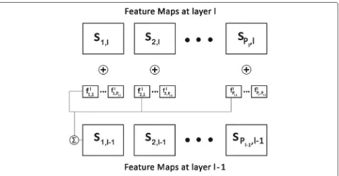
Deconvolutional network [31] is an unsupervised fea-ture learning model that is based on the convolutional decomposition of images under sparsity constraint and generates sparse, overcomplete features. Stacking such network in a hierarchy results in a deep deconvolutional network. Layers of such network learn both the filters and features as done in an image deconvolution problem in which given a degraded image, the task is to estimate both the blur kernel and the restored image. In order to explain how deep deconvolutional network extract hierar-chical features, we first consider a deep deconvolutional network consisting of a single layer. To train this network for extracting features, a training set consisting of large number of stereo imagesI={I1,. . .,Ims}_{are used where} each imageIi is considered as an input to the network. Here, ms is the number of images in the training setI, and we consider only left images of different scenes for training the network. Note that one may use right stereo images as well. LetP1be the number of 2Dfeature maps in a first layer. Considering the input at layer 0, we can write each imageIias composed ofP0channels{I₁i,. . .,I_Pi₀}. For example, if we consider a color image, then we haveP0=3. Each channelcof input imageIican be represented as a linear sum ofP1feature mapssipconvolved with filtersfp,c i.e.,

P1

p=1

si_p⊕fp,c=Ici, (5)

where ⊕ represents the 2D convolution operator. Note that in this work, we use gray scale stereo images only and henceP0= 1. Equation (5) represents an underdetermined system since both the features and filters are unknown and hence to obtain a unique solution, a regularization term is also added that encourages sparsity in the latent feature

maps. This gives us an overall cost function for training a single-layer deconvolutional network as:

C1(I)=

ms

i=1

⎡ ⎢ ⎣α 2 P0

c=1

P1

p=1

si_p⊕fp,c−Ici 2 2 + P1

p=1 |si_p|1

⎤ ⎥

⎦.

(6)

Here,|si_p|1is theL1-norm on the vectorized version of

si_p. The relative weighting of the reconstruction error of eachIiand sparsity of their feature mapssi_pis controlled by the parameterα. This network is learned by minimiz-ingC1(I)with respect tosi_ps andfp,cs when the input to network isI. Note that the set of filtersfp,care the param-eters of the network, common to all images in the training set while each image has its own set of feature mapssi

p. The single-layer network described above can be stacked to form a deep deconvolutional network consist-ing of multiple layers. Let the deep network is formed by

NL number of layers, (l = 1. . .NL). This hierarchy is achieved by considering the feature maps of layerl−1 as the input to layerl, l > 0. LetPl−1 andPl the number of feature maps at layerl−1 andl, respectively. The cost function for training the lth layer of a deep deconvolu-tional network can be written as a generalization of Eq. (6) as:

Cl(I)= ms

i=1

⎡ ⎢ ⎣α₂

Pl−1

c=1

Pl

p=1

g_pl_,_c(si_p_,_l⊕f_pl_,_c)−si_c_,_l₋₁ 2 2 + Pl

p=1 |si_p_,_l|1

⎤ ⎥ ⎦,

(7)

where si_c_,_l₋₁ andsi_p_,_l are the feature maps of imageIi at layer l − 1 and l, respectively, and thus, it shows that layerlhas as its input coming fromPl−1channels.fpl,care the filters at layerl and g_pl_,_c are the elements of a fixed binary matrix that determine the connectivity between the feature maps at successive layers, i.e., whethersi_p_,_l is connected to si_c_,_l₋₁ or not. For l = 1, we assume that

g_pl_,_cis always 1, but forl > 1, we make this connectivity as sparse. Since Pl > 1, the model learns overcomplete sparse, feature feature maps. This structure is illustrated in Fig. 1.

(6)

Fig. 1A deep deconvolutional network illustrating learning oflth layer

3.1 Feature encoding

Once the deep deconvolutional network is trained, we can use it to infer the multilayer features of a given leftILand rightIRstereo images for which we want to estimate the dense disparity map. The network described above is top-down in nature, i.e., given the latent feature maps, one can synthesize an image but there is no direct mechanism for inferring the feature maps of a given image without mini-mizing the cost function given in Eq. (7). Hence, once the network is learned/trained, we apply givenILandIR sepa-rately as input image to the trained deep deconvolutional network with the fixed set of learned filters and infer the feature mapssIL

p,l and s IR

p,l ofIL andIR at layerl, respec-tively, by minimizing the cost functionsCl(IL)andCl(IR), respectively. Once, they are learned, we create a feature vector at each pixel location in IL andIR separately. In order to obtain the features ofILat a layerl, we stack the

Pl number of inferred feature mapssI_pL_,_l and obtain a sin-gle feature mapZIL

l where at each pixel location(x,y)in

ZIL

l , we get a feature vector of dimensionPl×1. Similarly, using the same process we obtain the features ofIR. Thus,

ZIL l andZ

IR

l represents thelth layer features ofILandIR, respectively.

3.2 DefiningEF(d)

Once the multi-layer features ofILandIRare obtained, we can define our feature matching costEF(d)as:

EF(d)= NL

l=1

(x,y)

min

|ZIL

l (x,y)−Z IR

l (x+d(x,y),y)|,τ F_.

(8)

At each pixel location(x,y) having disparityd(x,y), it measures the absolute distance between the feature vec-torZIL

l (x,y) and corresponding matched featureZ IR l (x+

d(x,y),y). Here,τF _{is the truncation threshold which is} used to make feature matching cost more robust against outliers and NLis the number of layers in the network. These multiple layers feature matching technique highly constrains the solution space and hence results in unam-biguous and accurate disparities.

(7)

4 IGMRF model for disparity

Object distances from the camera, i.e., depths are inversely proportional to disparities and hence are made up of various textures, sharp discontinuities as well as smooth areas making them inhomogeneous. In our work, we use an IGMRF prior model which can adapt to the local structure of the disparity map, i.e., enforces the smooth-ness in disparities while preserving the discontinuities. IGMRF-based prior model has been successfully used in solving satellite image debluring problem [41], multireso-lution fusion of satellite images [48], and super-resomultireso-lution of images [49]. For modeling IGMRF,EIGMRF(d)is cho-sen as the square of finite difference approximation to the first-order derivative of disparities. Considering the differ-entiation in horizontal and vertical directions at each pixel location, one can writeEIGMRF(d)as [41]:

EIGMRF(d) =

(x,y)

bX₍_x_,_y₎(d(x−1,y)−d(x,y))2

+bY₍_x_,_y₎(d(x,y−1)−d(x,y))2. (9) Here, bX and bY are the spatially adaptive IGMRF parameters in horizontal and vertical directions, respec-tively. Thus,{bX₍_x_,_y₎,bY₍_x_,_y₎}forms a 2D parameter vector of IGMRF at each pixel location(x,y)in the disparity map. A low value ofbindicates the presence of an edge between two neighboring disparities. These parameters help us to obtain a solution which is less noisy in smooth areas and preserve the depth discontinuities in other areas. The IGMRF parameters at each pixel location(x,y) are esti-mated using the maximum likelihood estimation (MLE) and are computed as [41]:

bX₍_x_,_y₎= 1

max(4(d(x−1,y)−d(x,y))2, 4). (10)

bY₍_x_,_y₎= 1

max(4(d(x,y)−d(x,y−1))2, 4). (11) In order to avoid computational difficulty, we set an upper boundb = 1/4 whenever gradient becomes zero, i.e., whenever the neighboring disparities are the same.

In order to estimate IGMRF parameters, we need the true disparity map which is unknown and has to be esti-mated. Therefore, to start the regularization process, we use an initial estimate of disparity map obtained using a suitable approach and compute these parameters which are then used to estimate the d. In our proposed algo-rithm, these parameters and d are refined alternatively and iteratively for obtaining the betterd.

5 Sparse model for disparity

In order to model the higher order dependencies in the disparity map, we model the disparity map in our energy

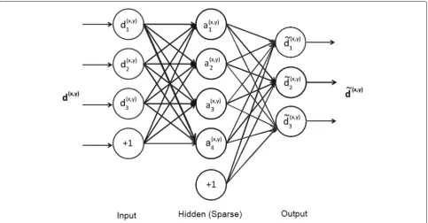
function by another prior called sparsity priorEsparse(d). The sparsity prior regularizes the solution by modeling the sparseness in d. In this work, we present a novel method for learning and inferring the sparse representa-tion of disparities using sparse autoencoder, which is then used to define the sparsity prior. An autoencoder is an artificial neural network (ANN) which sets the desired output same as the input and has one hidden layer [29]. It comprises of an encoder that maps an input vector to a hidden representation and a decoder that maps this hidden representation back to a reconstructed input. In reality, finding the sparse representation of a disparity map is computationally expensive, and therefore, a bet-ter choice would be to find the sparse representation of disparity patches of small size individually and average the resultant sparse patches at the end in order to get complete sparse representation of disparity map.

Let the input to an autoencoder be a disparity patch of size√n×√npixels, extracted at location(x,y)indand it is ordered lexicographically as column vectord(x,y) ∈Rn. Also, let the corresponding hidden representation ofd(x,y)

at hidden layer bea(x,y) ∈RK and the reconstructed out-put be d˜(x,y) ∈ Rn. Thus, the number of units at input, hidden, and output layers aren,K, andn, respectively. The autoencoder has weights(W,U,r,s), whereW ∈Rn×K is the encoder weight matrix between the input and hidden layers,U ∈ RK×nis the decoder weight matrix between the hidden and output layers, andr ∈ RK ands ∈ Rn

are the bias weight vectors for hidden and output lay-ers, respectively. For a fixed set of weights(W,U,r,s), the

a(x,y)_and_d˜(x,y)_{can be computed as follows:}

a(x,y)=f

WTd(x,y)+r

, (12)

˜

d(x,y)=f

UTa(x,y)+s

, (13)

wheref is an activation function and we use sigmoid for this. An autoencoder is called as sparse autoencoder when the sparsity constraint is imposed on its hidden layer. Sparse autoencoder learns an overcomplete sparse repre-sentation of data in the hidden layer when the number of hidden unitsK are greater than the number of input unitsn, i.e.,K>n. An example of a sparse autoencoder is shown in Fig. 2.

(8)

Fig. 2A sparse autoencoder withn=3 andK=4. Here +1 represents a bias unit

for each jth hidden unit is enforced by a penalty term which penalizesρˆjdeviating significantly fromρas:

K

j=1

KL(ρ|| ˆρj)= K

j=1 ρlogρ

ˆ ρj+(

1−ρ)log 1−ρ 1− ˆρj

, (14)

whereKL(ρ|| ˆρj)is the Kullback-Leilbler (KL) divergence. This term has a value 0, ifρˆj=ρ; otherwise, it increases monotonically asρˆjdiverges fromρ.

Consider a training set consisting of large number of disparity patchesG={d(1),d(2),. . .,d(md)}_{, with each patch}

d(i) ∈ Rn. One can extract these disparity patches from the available ground truth disparity maps. Using the known disparity patches, we can train the sparse autoen-coder to learn the weights (W,U,r,s). To do this, the following objective function is formed using Eqs. (12), (13), and (14) as:

1

m

md

i=1

1 2

d(i)−fUTf WTd(i)+r+s2

2

+λ

2 ⎛

⎝n

i=1 K

j=1

(Wij)2+ K

i=1 n

j=1 (Uij)2

⎞ ⎠

+β K

j=1

KL(ρ|| ˆρj). (15)

Here, the first term represents the average reconstruc-tion error over all training inputs. The second term is a

regularization term on the weights to prevent the over-fitting by making them smaller in magnitude, andλ con-trols the relative importance of this term.β controls the weightage of the third term which corresponds to sparsity penalty term. We minimize this Eq. (15) w.r.t.W,U,r,s

using well known back propagation algorithm [50]. Once the autoencoder is trained,dcan be modeled by the sparsity priorEsparse(d)as follows:

Esparse(d)=

(x,y)

d(x,y)−fUTa(x,y)+s2

2. (16)

Esparse(d) measures how well each disparity patch at location (x,y) in d agrees with its sparse representa-tions. In our proposed approach, the disparity map and its sparse representation are inferred alternatively.

6 Dense disparity estimation

E(d)=

(x,y)

min

d(x,y)±1 2

IL(x,y)−IR(x+d(x,y),y)

,τI

+μ NL

l=1

(x,y)

minZIL

l (x,y)−Z IR

l (x+d(x,y),y),τF

+

(x,y)

bX₍_x_,_y₎(d(x−1,y)−d(x,y))2+bY₍_x_,_y₎(d(x,y−1)

−d(x,y))2+γ

(x,y)

d(x,y)−fUTa(x,y)+s2 2.

(9)

Our main goal is to estimate the dense disparity map using a given pair of stereo images in an energy mini-mization framework. Our data term defined in Eq. (2) is formed by adding intensity and feature matching costs using Eqs. (3) and (8), respectively. Similarly, our prior energy term defined in Eq. (4) is formed by adding the IGMRF and sparsity priors using Eqs. (9) and (16), respec-tively. Finally, our proposed energy function defined in Eq. (1) can be rewritten as given in Eq. (17) and we minimize it using graph cuts optimization based on α-β swap moves [7]. We do not consider the occlu-sions explicitly but they are handled by clipping match-ing costs usmatch-ing thresholds τ = {τI_,_τF_} _{that prevents} the outliers from disturbing the estimation (see Eqs. (3) and (8)).

In order to estimate the dense disparity map, we pro-pose an iterative two-phase algorithm. It proceeds with the use of an initial estimate of disparity map and iter-ates and alterniter-ates between two phases until conver-gence as given in Algorithm 1. We use a classical local stereo method [1] for obtaining the initial disparity map in which the absolute intensity differences (AD) with truncation, aggregated over a fixed window is used as matching cost. In order to reduce computation time, we optimize this cost by graph cuts instead of the clas-sic winner take all (WTA) optimization. Postprocessing operations such as left-right consistency check, interpo-lation, and median filtering [1] are applied in order to obtain a better initial estimate for faster convergence while regularizing. However, any other suitable disparity esti-mation method can also be used in obtaining the initial estimate.

Algorithm 1:Proposed algorithm

Input: Stereo image pairILandIR, a set of ground truth

disparity patchesG={d(1),d(2),. . .,d(md)}_{, and a set} of stereo imagesI={I1,. . .,Ims}_.

1 Train a sparse autoencoder usingGby minimizing Eq.(15) and obtain weights(W,U,r,s);

2 Train a deep deconvolutional network consisting ofNL number of layers, by minimizing Eq.(7) for each layerland learn a set of filters;

3 Infer the multi-layer featuresZI_lLandZ_lIRofILandIR,

respectively (l=1. . .NL); 4 Obtain an initial disparity mapd0;

5 Initialization:d=d0;

6 repeat

7 Phase 1:Withdbeing fixed, infer the sparse vector

a(x,y)_{for each disparity patch}_d(x,y)_in_d_{using Eq.(12).}

Compute IGMRF parametersbX₍_x_,_y₎andbY₍_x_,_y₎using Eqs.(10) and (11), at each pixel location;

8 Phase 2: With{a(x,y)},{b₍X_x_,_y₎,bY₍_x_,_y₎}fixed as obtained in phase 1, minimize the Eq.(17) fordusing graph cuts; 9 untilconvergence;

In general, for nonconvex energy functions, graph cuts result in a local minimum that is within a known factor of global minimum. In order to ensure global minimum, we use an iterative optimization with proper settings of parameters. At every iteration, the IGMRF parameters and sparseness are refined in order to obtain better dis-parity estimates (converging towards global optima). The number of iterations may vary for different stereo pairs and the choice of initial estimate.

7 Experimental results

In this section, we demonstrate the efficacy of the pro-posed method by conducting various experiments and evaluating our results on the Middlebury stereo bench-mark images [2]. In order to perform the quantitative evaluation, we use the percentage of bad matching pixels (B%) as the error measure with a disparity error tolerance δ. The error measure is computed over the entire image as well as in the nonoccluded regions. For an estimated disparity mapd, theB%is computed with respect to the ground truth disparity mapgas follows [1]:

B= 1 M∗N

(x,y)

|d(x,y)−g(x,y)|> δ, (18)

In this work, all the experiments were conducted on a computer with Core i7-3632QM, 2.20 GHz processor and 8.00 GB RAM.

7.1 Parameter settings

We first provide the details of various parameters used in training the deep deconvolutional network. A two-layer deep deconvolutional network was trained overms=75 left stereo images obtained from the Middlebury 2005 and 2006 datasets and Middlebury 2014 training dataset [2]. Considering NL = 2 i.e., for a two-layer deep architec-ture, we set the number of feature maps as P1 = 9 and

(10)

Fig. 3Filters learned at first and second layers of deep deconvolutional network.aNumber of filters learned at first layer are 9.bNumber of filters learned at second layer are 81 where 36 filters in pair are shown in color and remaining 9 filters are shown asgrayscale

We now provide the parameters used while training the sparse autoencoder. We trained the sparse autoencoder using a set of md = 5 × 105 true disparity patches of the stereo images used during the training of deep decon-volutional network. The size of each disparity patch was chosen as 8×8, i.e.,n= 64. In order to achieve the over-completeness in hidden layer, we set K=4 ∗n, i.e., the number of hidden units wereK= 256. The parameters in Eq. (15) were empirically chosen asλ = 10−4_,_β ₌ _0.1, andρ = 0.01. With these parameter settings, the sparse autoencoder was trained to obtain the weights(W,U,r,s). The learned weightsWbetween the input and the hidden layers are shown in Fig. 4.

Fig. 4Learned weightsWbetween the input and the hidden layer in the trained sparse autoencoder. Here, each square block is of size 8_×8 which shows the weights between a hidden unit and each input unit. Note that there are 256 hidden and 64 input units

Note that the training of deep deconvolutional network and the autoencoder is an offline operation, and hence, they do not add to the computational complexity. In order to estimate the dense disparity map, we experimented on the Venus, Cones, and Teddystereo pairs, belonging to Middlebury stereo 2001 and 2003 datasets [2] which were different from the training datasets used earlier. We also performed the experiments using the recently released Middlebury stereo 2014 (version 3) dataset. Our algo-rithm was initialized with the initial estimate of disparity map and the algorithm converged with in five iterations for all the stereo pairs used in our experiments. While minimizing Eq. (17), the data cost thresholds{τI,τF}were set as 0.08 and 0.04, respectively, and the parameter μ was chosen as 1. The parameter γ was initially set to 10−4and exponentially increased at each iteration from 10−4 to 10−1. We used the same parameters for all the experiments, and this demonstrates the robustness of our method.

7.2 Performance evaluation using different data terms

ED(d)with IGMRF prior

As discussed earlier, the data term ED(d) in our energy function is defined using a combination of EI(d) and

EF(d). In order to demonstrate the effectiveness of our proposed data term, we consider the energy functions consisting of different data termsED(d)and IGMRF prior only. Note that we do not consider the sparsity prior here. We then compare the performance using the proposed

(11)

Table 1Performance evaluation in terms of percentage of bad matching pixels computed over the whole image withδ= 1. Here, the optimization of energy function is carried out using different data termsED(d)with IGMRF as prior termEP(d)

ED(d) Venus Teddy Cones

AD 1.90 16.49 12.14

BT 0.95 15.67 11.89

BT+gradient 0.89 14.9 11.32

EI(d)+EF(d) 0.40 11.41 9.98

of the other methods are also used with truncation on their costs. The results of these experiments are summa-rized in Table 1. The results show that the approach using proposedED(d)outperforms those with traditional pixel-basedED(d). These results show the effectiveness of using the learning-based multilayer feature matching costEF(d) in our approach. In other words, when the intensity and the learning-based feature matching are combined, the estimated disparities are more robust and accurate. The results also show that data term defined using the deep-learned features gives better disparities as compared to the one which uses basic gradient features.

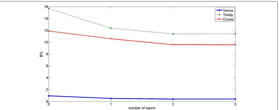
We now demonstrate the performance of our approach by varying the number of layers in the feature match-ing costEF(d). Once again, we consider the same energy function consisting of data termED(d)and IGMRF prior where ED(d) is defined using EI(d) andEF(d). We first obtained the disparity map whenEF(d)is defined using the learned features of first layer only. Next, the results are obtained whenEF(d)is defined using the learned features of both first and second layers. In other words, we con-sider NL = 1 and NL = 2 in Eq. (8) for these two cases. Figure 5 shows that the performance improves when we

use two-layer feature matching. We also experimented with the use of three layers but we did not find significant improvement when the number of layers NL is greater than 2 (see Fig. 5). Based on these observations, we used only two-layer deep deconvolutional network in our work. This shows the effectiveness of the use of deep learning with limited number of layers.

7.3 Performance evaluation using different prior terms

EP(d)with proposedED(d)

As discussed earlier, the prior termEP(d)in our energy function is defined using the combination of IGMRF and sparsity priors. We consider the energy function con-sists of proposed data termED(d)andEP(d)and evaluate the performance of our approach using different choices of EP(d). For doing the same, we first chooseEP(d) as

EIGMRF(d)and compare by choosing other discontinuity preserving MRF priors such as truncated quadratic, trun-cated linear, and Potts models. The results in Table 2 show that the approach using the IGMRF prior combined with proposedED(d)performs significantly better when com-pared to the use of other discontinuity preserving priors. This shows the effectiveness of using IGMRF prior since it better captures the spatial variation among disparities. We then evaluate the performance by choosingEP(d)as a combination ofEIGMRF(d) andEsparse(d). For this, we consider three cases. In the first case, the Esparse(d) is obtained using the fixed DCT bases, in the second case, it is learned using the K-SVD dictionary learning method, and in the last case, we define the Esparse(d) using the proposed sparse autoencoder. As seen from the Table 2, the results are significantly improved when the sparsity prior is combined with the IGMRF prior and the proposed data term. This is expected because IGMRF and spar-sity priors together capture the disparity characteristics

(12)

Table 2Performance evaluation using different prior termsEP(d) with proposedED(d). The errors are shown in terms of bad matching pixels and these are computed over the whole image withδ=1

EP(d) Venus Teddy Cones

Truncated quadratic 1.95 15.38 11.62

Truncated linear 0.91 12.86 10.96

Potts 1.11 13.93 11.01

EIGMRF(d) 0.40 11.41 9.64

EIGMRF(d)+Esparse(d)using DCT 0.38 11.1 9.36

EIGMRF(d)+Esparse(d)using K-SVD 0.30 10.60 9.12

EIGMRF(d)+Esparse(d)using autoencoder 0.20 9.76 8.46

in different ways and their combination serves as a better regularizer. The results also show that the use of spar-sity prior obtained using proposed sparse autoencoder perform better when compared to those obtained using K-SVD or fixed basis. This is because the sparseness is better captured by the learned weights of autoencoder.

7.4 Qualitative and quantitative assessment and comparison with state of the art methods

Here, we first show the qualitative and quantitative perfor-mances of our algorithm experimented using Middlebury stereo 2001 and 2003 datasets [2]. Figure 6 shows the estimated disparity maps of the proposed approach using these datasets. One can see that the final disparity maps

are piecewise smooth and visually plausible. We also dis-play the error maps associated with the final disparity maps as shown in the last column of Fig. 6. The error maps show the regions where the estimated disparities differ from the ground truth (black and gray regions cor-respond to errors in occluded and non occluded regions, respectively and white indicates no error). We can see that the proposed method has higher accuracy in discontinu-ous as well as nonoccluded regions. This is because the IGMRF prior preserves the discontinuities and the spar-sity prior learns the edge-like sparse features in disparity map, and using these two with the proposed data term produces accurate disparities. As can be seen from Fig. 6, our method not only preserves geometrical details near depth discontinuities but performs better in textureless regions as well. We mention here that although we do not consider occlusions in our problem formulation, our method works well in these regions as well. Performance improvement in occluded regions is due to the presence of data term truncation thresholds, i.e.,τ ={τI,τF}.

The quantitative assessment of our algorithm experi-mented using Middlebury stereo 2001 and 2003 datasets [2] is shown in Table 3. In order to validate the results of our method, we compare it with state-of-the-art global dense stereo methods in terms of percentage of bad matching pixels (B%). The compared approaches include feature based [16–18] and regularization based such as MRF priors [36–39], Mumford Shah regularization [51], ground control points [52], learned conditional random field (CRF) [53], and sparsity prior [42, 46] methods.

Fig. 6Experimental results for the Middlebury stereo 2001 and 2003 datasets [2],Venus(first row),Teddy(second row), andCones(third row). The left imageILand the ground truth disparity map are shown infirst and second columns, respectively. Thethird columnshows the initial disparity map

(13)

Table 3Quantitative evaluation on Middlebury stereo 2001 and 2003 datasets [2] and comparison with state-of-the-art global dense stereo methods in terms of bad matching pixels over entire image as well as non occluded regions withδ= 1

Method Venus Teddy Cones

All Nonocc All Nonocc All Nonocc

Initial 3.47 2.00 19.65 5.61 16.43 7.15

Proposed 0.20 0.10 9.76 3.44 8.46 2.36

AdaptBP [16] 0.21 0.10 7.06 4.22 7.92 2.48

DoubleBP [38] 0.45 0.13 8.30 3.53 8.78 2.90

GCP [52] 0.53 0.16 11.5 6.44 9.49 3.59

TwoStep [17] 0.45 0.27 12.6 7.42 10.1 4.09

SemiGlob [18] 1.57 1.00 12.2 6.02 9.75 3.06

2OP [39] 0.49 0.24 15.4 10.9 10.8 5.42

CompSens [42] 0.68 0.31 13.30 7.88 9.79 3.97

MultiGC [37] 3.13 2.79 17.6 12.0 11.8 4.89

Mumford [51] 0.76 0.28 14.3 9.34 9.91 4.14

GC [36] 3.44 1.79 25.0 16.5 18.2 7.70

CRF [53] 1.3 – 11.1 – 10.8 –

Sparse [46] – – 11.98 – 8.14 –

Here,en dashindicates the result not reported. First row shows the results using initial estimate

These results are compared without using any post pro-cessing operations. We do not compare our method with global stereo methods based on handcrafted and learned features [19–21, 27] since their results are not available for the Middlebury datasets. As seen from the Table 3, our method performs best among all the other methods in nonoccluded regions. It also gives least bad match-ing pixels over entire image as well as in nonoccluded regions for the Venus stereo pair. We see that the over-all performance of the proposed method is comparable

to state-of-the-art global stereo methods. The results also indicate the effectiveness of the proposed energy function in the global energy minimization framework for dense disparity estimation.

Finally, we show the qualitative and quantitative per-formance of our algorithm experimented on Middlebury stereo 2014 datasets [2] that consists of 15 training and 15 test stereo pairs. Figure 7 shows the estimated dis-parity maps of the proposed approach using some of these datasets. In order to validate and compare the

(14)

performance of our method with other latest stereo meth-ods listed on [2], we submitted these estimated disparity maps online to the server available on Middlebury website [2] which in turn returned the overall evaluation and com-parison chart. Since the test dataset does not have ground truth, evaluation is only done by submitting the estimated disparity maps on this online server. We mention here that one cannot adjust the parameters for test datasets because the submission can be done only once. The quali-tative and quantiquali-tative results and the comparisons can be seen on Middlebury stereo evaluation page. We achieve a ranking of 43 for training set and ranking of 48 on test set. Our method does not rank among the top methods because the accuracy of our method is sensitive to the parameters of the model. One can enhance the results by carefully choosing the parameters. Experimental results indicate that our method is better than the state-of-the-art regularization-based methods and comparable to other latest stereo methods.

8 Conclusion

We have presented a new approach for dense disparity map estimation based on inhomogeneous MRF and spar-sity priors in an energy minimization framework. The data term is defined using the combination of intensity and the learning-based multilayer feature matching costs. The feature matching cost is defined over the deep learned features of given stereo pair, and we have used deep deconvolutional network for learning these hierarchical features. The IGMRF prior captures the smoothness in disparities and preserves the discontinuities in terms of IGMRF parameters. The sparsity prior is defined over the learned sparseness of disparities where the sparse rep-resentation of disparities are learned using the sparse autoencoder. We have presented an iterative two-phase algorithm for disparity estimation where in phase one, the disparity map is estimated by minimizing our energy function using graph cuts and in phase two, the IGMRF parameters and sparse representation of disparity maps are obtained. Experiments conducted on various datasets of Middlebury site verify the effectiveness of the pro-posed data term, IGMRF, and sparsity priors when used in an energy minimization framework. Performance of the proposed method is comparable to many of the better performing and latest dense stereo methods.

Authors’ contributions

Both authors have equally contributed to the manuscript. Both authors read and approved the final manuscript.

Authors’ information

Sonam Nahar received the B.E. degree in Information Technology from Manikya Lal Verma Textile Enginerring College, Bhilwara, India, in 2008, and M.Tech. degree in Information and Communication Technology from Dhirubhai Ambani Institute of Information and Technology (DA-IICT), Gandhinagar, India, in 2010. She is currently pursuing the Ph.D degree from DA-IICT, Gandhinagar, India, and serving as an Assistant Professor with The

Laxmi Niwas Mittal Institute of Information Technology (LNMIIT), Jaipur, India, in Computer Science and Engineering Department. Her research interests include computer vision, image processing, and deep learning. Manjunath V. Joshi received the B.E. degree from the University of Mysore, Mysore, India, and the M.Tech. and Ph.D. degrees from the Indian Institute of Technology Bombay (IIT Bombay), Mumbai, India. Currently, he is serving as a Professor with the Dhirubhai Ambani Institute of Information and Communication Technology, Gandhinagar, India. He has been involved in active research in the areas of signal processing, image processing, and computer vision. He has coauthored two books entitled Motion-Free Super Resolution (Springer, New York) and Digital Heritage Reconstruction Using Super resolution and Inpainting (Morgan and Claypool). Dr. Joshi was a recipient of the Outstanding Researcher Award in Engineering Section by the Research Scholars Forum of IIT Bombay. He was also a recipient of the Best Ph.D. Thesis Award by Infineon India and the Dr. Vikram Sarabhai Award in the field of information technology constituted by the Government of Gujarat, India.

Competing interests

The authors declare that they have no competing interests.

Author details

1_{The LNM Institute of Information Technology, Jaipur, India.}2_Dhirubhai

Ambani Institute of Information Technology, Gandhinagar, India.

Received: 15 April 2016 Accepted: 27 December 2016

References

1. Scharstein D, Szeliski R, Zabih R (2002) A taxonomy and evaluation of dense two-frame stereo correspondence algorithms. Int J Comput Vis 47(1/2/3):7–42

2. Scharstein D, Szeliski R, Zabih R (1987) Middlebury Stereo. http://vision. middlebury.edu/stereo

3. Kanade T, Okutomi M (1994) A stereo matching algorithm with an adaptive window: theory and experiment. Pattern Anal Mach Intell IEEE Trans 16(9):920–932

4. Fusiello A, Roberto V, Trucco E (1997) Efficient stereo with multiple windowing. In: Proceedings of IEEE Computer Society Conference on Computer Vision and Pattern Recognition. pp 858–863.

doi:10.1109/CVPR.1997.609428

5. Yoon KJ, Kweon IS (2006) Adaptive support-weight approach for correspondence search. Pattern Anal Mach Intell IEEE Trans 28(4):650–656 6. Hosni A, Rhemann C, Bleyer M, Rother C, Gelautz M (2013) Fast

cost-volume filtering for visual correspondence and beyond. Pattern Anal Mach Intell IEEE Trans 35(2):504–511

7. Kolmogorov V, Zabih R (2004) What energy functions can be minimized via graph cuts? Pattern Anal Mach Intell IEEE Trans 26(2):147–159 8. Sun J, Zheng NN, Shum HY (2003) Stereo matching using belief

propagation. Pattern Anal Mach Intell IEEE Trans 25(7):787–800 9. Tappen MF, Freeman WT (2003) Comparison of graph cuts with belief

propagation for stereo, using identical MRF parameters, vol.2. In: Proceedings Ninth IEEE International Conference on Computer Vision Vol. 2. pp 900–906. doi:10.1109/ICCV.2003.1238444

10. Hirschmuller H, Scharstein D (2007) Evaluation of cost functions for stereo matching. In: 2007 IEEE Conference on Computer Vision and Pattern Recognition. pp 1–8. doi:10.1109/CVPR.2007.383248

11. Tola E, Lepetit V, Fua P (2010) Daisy: An efficient dense descriptor applied to wide-baseline stereo. Pattern Anal Mach Intell IEEE Trans 32(5):815–830 12. Joglekar J, Gedam SS, Mohan BK (2014) Image matching using sift

features and relaxation labeling technique:a constraint initializing method for dense stereo matching. Geosci Remote Sensing, IEEE Trans 52(9):5643–5652

13. Grimson WEL (1985) Computational experiments with a feature based stereo algorithm. Pattern Anal Mach Intell IEEE Trans 7(1):17–34 14. Ayache N, Faverjon B Efficient registration of stereo images by matching

graph descriptions of edge segments. International Journal of Computer Vision:107–131

(15)

16. Klaus A, Sormann M, Karner K (2006) Segment-based stereo matching using belief propagation and a self-adapting dissimilarity measure, vol.3. In: 18th International Conference on Pattern Recognition (ICPR’06). pp 15–18. doi:10.1109/ICPR.2006.1033

17. L. Wang ZL, Zhang Z (2014) Feature based stereo matching using two-step expansion. Math Probl Eng 14:14

18. Hirschmüller H (2008) Stereo processing by semi-global matching and mutual information. Pattern Anal Mach Intell IEEE Trans 30(2):328–341 19. Liu C, Yuen J, Torralba A (2011) Sift flow: dense correspondence across

scenes and its applications. Pattern Anal Mach Intell IEEE Trans 33(5):978–994 20. Kim J, Liu C, Sha F, Grauman K (2013) Deformable spatial pyramid

matching for fast dense correspondences. In: 2013 IEEE Conference on Computer Vision and Pattern Recognition. pp 2307–2314.

doi:10.1109/CVPR.2013.299

21. Saxena A, Chung SH, Ng AY (2007) 3-D depth reconstruction from a single still image. Int J Comput Vis 76:2007

22. Vincent P, Larochelle H, Lajoie I, Bengio Y, Manzagol P (2010) Stacked denoising autoencoders: learning useful representations in a deep network with a local denoising criterion. J Mach Learn Res 11:3371–3408 23. Krizhevsky A, Sutskever I, Hinton GE (2012) Imagenet classification with

deep convolutional neural networks. In: Advances in Neural Information Processing Systems 25. pp 1097–1105

24. Bengio Y (2009) Learning deep architectures for AI. Foundations Trends Mach Learn 2(1):1–127

25. Dong C, Loy CC, He K, Tang X (2015) Image super-resolution using deep convolutional networks. CoRR abs/1501.00092

26. Zbontar J, LeCun Y (2014) Computing the stereo matching cost with a convolutional neural network. CoRR abs/1409.4326

27. Zhang C, Shen C (2015) Unsupervised feature learning for dense correspondences across scenes. CoRR abs/1501.00642 28. Poultney C, Chopra S, Lecun Y (2006) Efficient learning of sparse

representations with an energy-based model. In: Advances in Neural Information Processing Systems

29. Lee H, Ekanadham C, Ng AY (2007) Sparse deep belief net model for visual area v2. In: Neural Information Processing Systems. pp 873–880 30. Hinton GE, Osindero S (2006) A fast learning algorithm for deep belief

nets. Neural Comput 18:2006

31. Zeiler MD, Krishnan D, Taylor GW, Fergus R (2010) Deconvolutional networks. In: 2010 IEEE Computer Society Conference on Computer Vision and Pattern Recognition. pp 2528–2535. doi:10.1109/CVPR.2010.5539957 32. Zeiler MD, Taylor GW, Fergus R (2011) Adaptive deconvolutional networks

for mid and high level feature learning. In: Computer Vision, IEEE International Conference On. pp 2018–2025

33. Jarrett K, Kavukcuoglu K, Ranzato MA, Lecun Y (2009) What is the best multi-stage architecture for object recognition? In: 2009 IEEE 12th International Conference on Computer Vision. pp 2146–2153. doi:10.1109/ICCV.2009.5459469

34. Li SZ (1995) Markov random field modeling in computer vision. Springer, New York

35. Roy S (1999) Stereo without epipolar lines: a maximum-flow formulation. Int J Comput Vis 34(2–3):147–161

36. Boykov Y, Veksler O, Zabih R (2001) Fast approximate energy minimization via graph cuts. Pattern Anal Mach Intell IEEE Trans 23(11):1222–1239 37. Kolmogorov V, Zabih R (2002) Multi-camera scene reconstruction via

graph cuts. In: Computer Vision, European Conference On. pp 82–96 38. Yang Q, Wang L, Yang R, Stewenius H, Nister D (2009) Stereo matching

with color-weighted correlation, hierarchical belief propagation, and occlusion handling. Pattern Anal Mach Intell IEEE Trans 31(3):492–504 39. Woodford O, Torr P, Reid I, Fitzgibbon A (2008) Global stereo

reconstruction under second order smoothness priors. In: Computer Vision and Pattern Recognition, IEEE Conference On. pp 1–8 40. Zhang L, Seitz SM (2005) Parameter estimation for MRF stereo, vol.2. In:

2005 IEEE Computer Society Conference on Computer Vision and Pattern Recognition (CVPR’05), Vol. 2. pp 288–295. doi:10.1109/CVPR.2005.269 41. Jalobeanu A, Blanc-Feraud L, Zerubia J (2004) An adaptive gaussian model

for satellite image deblurring. Image Process IEEE Trans 13(4):613–621 42. Hawe S, Kleinsteuber M, Diepold K (2011) Dense disparity maps from

sparse disparity measurements. In: 2011 International Conference on Computer Vision. pp 2126–2133. doi:10.1109/ICCV.2011.6126488

43. Elad M, Aharon M (2006) Image denoising via sparse and redundant representations over learned dictionaries. Image Process IEEE Trans 15(12):3736–3745

44. Xie J, Xu L, Chen E (2012) Image denoising and inpainting with deep neural networks. In: Advances in Neural Information Processing Systems 25. pp 350–358

45. Aharon M, Elad M, Bruckstein A (2006) K -SVD: An algorithm for designing overcomplete dictionaries for sparse representation. Signal Process IEEE Trans 54(11):4311–4322

46. Tosic I, Olshausen BA, Culpepper BJ (2011) Learning sparse representations of depth. Selected Topics Signal Process IEEE J 5(5):941–952

47. Birchfield S, Tomasi C (1998) A pixel dissimilarity measure that is insensitive to image sampling. Pattern Anal Mach Intell IEEE Trans 20(4):401–406 48. Joshi M, Jalobeanu A (2010) Map estimation for multiresolution fusion in

remotely sensed images using an IGMRF prior model. Geosci Remote Sensing IEEE Trans 48(3):1245–1255

49. Gajjar PP, Joshi MV (2010) New learning based super-resolution: use of DWT and IGMRF prior. Image Process IEEE Trans 19(5):1201–1213 50. Mitchell TM (1997) Machine learning. McGraw-Hill, New York, USA 51. Ben-Ari R, Sochen N (2010) Stereo matching with Mumford-Shah

regularization and occlusion handling. Pattern Anal Mach Intell IEEE Trans 32(11):2071–2084

52. Wang L, Yang R (2011) Global stereo matching leveraged by sparse ground control points. In: CVPR 2011. pp 3033–3040.

doi:10.1109/CVPR.2011.5995480

53. Scharstein D, Pal C (2007) Learning conditional random fields for stereo. In: Computer Vision and Pattern Recognition, IEEE Conference On. pp 1–8