R E S E A R C H
Open Access
A resource management technique for
processing deadline-constrained
multi-stage workflows
Norman Lim
1*, Shikharesh Majumdar
1and Peter Ashwood-Smith
2Abstract
The use of cloud computing that provides resources on demand to various types of users, including enterprises as well as engineering and scientific institutions, is growing rapidly. An effective resource management middleware is necessary to harness the power of the underlying distributed hardware in a cloud. Two of the key operations provided by a resource manager are resource allocation (matchmaking) and scheduling. This paper concerns the problem of matchmaking and scheduling an open stream ofmulti-stage jobs(orworkflows) with Service Level Agreements (SLAs) on a cloud or cluster. Multi-stage jobs require service from multiple system resources and are characterized by multiple phases of execution. This paper presents a resource allocation and scheduling technique called RM-DCWF: Resource Management Technique for Deadline-constrained Workflows that can efficiently matchmake and schedule an open stream of multi-stage jobs with SLAs, where each SLA is characterized by an earliest start time, an execution time, and a deadline. A rigorous simulation-based performance evaluation of RM-DCWF is conducted using synthetic workloads derived from real scientific workflows. In addition, the impact of various system and workload parameters on system performance is investigated. The results of this performance evaluation demonstrate the effectiveness of RM-DCWF as captured in a low number of jobs missing their deadlines.
Keywords:Resource allocation and scheduling on clouds, Multi-stage jobs with SLAs, Workflows with SLAs, Jobs with deadlines
Introduction
Over the past few years, distributed computing para-digms such as cluster computing and cloud computing have been generating a lot of interest among consumers and service providers as well as researchers and system builders. For example, a number of reputable financial institutions and market research organizations have predicted a multi-billion-dollar market for the cloud computing industry [1, 2]. An important feature of cloud computing is that it allows users to acquire resources on demand and pay only for the time the resources are used. Investigating and devising effectiveresource management techniquesfor clouds and clusters is necessary to harness the power of the underlying distributed hardware and to achieve the performance objectives of a system [3], which
can include generating high job throughput and low job response times, meeting the quality of service (QoS) re-quirements of jobs that are often captured by a service level agreement (SLA), and maintaining a high resource utilization to generate adequate revenue for the cloud service provider. As in the case of grids, a predecessor of cloud computing that also supported resources on de-mand, QoS and satisfying SLAs remain an important issue for cloud computing [3, 4]. Handling of jobs with a SLA often leads to an advance reservation request [5] that is characterized by an earliest start time, a required execu-tion time, and adeadlinefor completion. This is of critical importance for latency-sensitive business and scientific applications that can include live business intelligence and sensor-based applications which rely on a timely process-ing of the collected data. Two of the key operations that a resource manager needs to provide areresource allocation (matchmaking) and scheduling. Note that the matchmak-ing and schedulmatchmak-ing operations are jointly referred to as * Correspondence:[email protected]
1Department of Systems and Computer Engineering, Carleton University,
Ottawa, ON, Canada
Full list of author information is available at the end of the article
mapping operation [6]. Given a pool of resources, the matchmaking algorithm chooses the resource(s) to be allocated to an incoming job. Once a number of jobs are allocated to a specific resource, a scheduling algorithm determines the order in which jobs allocated to the re-source should be executed for achieving the desired system objectives. Performing effective matchmaking and scheduling is difficult because the SLA of the jobs need to be satisfied, while also considering system ob-jectives, which can include minimizing the number of jobs that miss their deadlines as well as generating ad-equate revenue for the service provider.
Due to cloud computing becoming more prevalent, a variety of applications are being run on clouds, includ-ing those that are characterized by multiple phases of execution and require processing from multiple system resources (referred to asmulti-stage jobs). Scientific ap-plications and workflows that are used in various fields of study, such as physics and biology, are examples of multi-stage jobs that are run on clouds. Moreover, an-other example of a popular multi-stage application that is typically run on clouds is MapReduce [7], which is a programming model (proposed by Google) for simplifying the processing of very large and complex data sets in a parallel manner. MapReduce is used by many companies and institutions, typically in conjunction with cloud or cluster computing, for facilitating Big Data analytics [8–10]. The focus of this paper is to devise an efficient matchmaking and scheduling technique for processing an open stream of multi-stage jobs (workflows) with SLAs on a distributed computing environment with a fixed number of resources (e.g. a private cluster or a set of resources acquired a priori from a public cloud). Most existing research focuses on meeting the SLA for jobs that require processing from only a single resource or handling of a fixed number of multi-stage jobs exe-cuting on the system. There is comparatively less work available in the literature focusing on resource manage-ment for a workload comprising and open stream of multi-stage jobs with SLAs. Handling of an open stream of multi-stage jobs increases the complexity of the resource allocation and scheduling problem due to a continuous stream of jobs arriving on the system. Thus, the novel matchmaking and scheduling tech-niques described in this paper are expected to make a significant contribution to the state of the art.
This paper presents a novel resource allocation and scheduling technique, referred to as RM-DCWF: Resource Management Technique for Deadline-constrained Work-flows, that can effectively perform matchmaking and sched-uling for an open stream of multi-stage jobs with SLAs, where each SLA comprises an earliest start time, an execu-tion time, and an end-to-end deadline. RM-DCWF decom-poses the end-to-end deadline of a job into components
(i.e. sub-deadlines), each of which is associated with a task in the job. The individual tasks of the job are then mapped on to the resources where the objective is to satisfy the job’s SLA and minimize the number of jobs that miss their deadlines. In our preliminary work [11], a resource allocation and scheduling technique for pro-cessing deadline-constrained MapReduce [7] jobs (com-prising of only two phases of execution) is described. The algorithm described in [11] can only handle MapReduce jobs. The algorithm presented in this paper is new as it focuses on a more complex resource man-agement problem that considers jobs and workflows characterized by multiple (two or more) phases of exe-cution as present in scientific workflows, for example. Furthermore, the jobs handled by the algorithm intro-duced in this paper can have various structures charac-terized by different precedence relationships among the respective constituent tasks that are not considered in [11]. To the best of our knowledge, none of the existing work focuses on all aspects of the resource manage-ment problem that this paper focuses on: devising a re-source allocation and scheduling algorithm for multi-stage jobs with SLAs on a system subjected to an open stream of job arrivals. The main contributions of this paper include:
A novel resource allocation and scheduling technique, RM-DCWF, for handling an open stream of multi-stage jobs with SLAs. Two task scheduling policies are devised.
Two algorithms devised to decompose the end-to-end deadline of a multi-stage job to assign each task of the job a sub-deadline.
Insights gained into system behavior and performance from a rigorous simulation-based performance evaluation of RM-DCWF using a variety of system and workload parameters. The synthetic workloads used in the experiments are based on real scientific workflows described in the literature.
A comparison of the performance of the proposed technique with that of a conventional first-in-first-out (FIFO) scheduler as well as a technique from the literature [29] that has objectives similar to RM-DCWF is presented.
and scheduling algorithms are presented. The results of the performance evaluation of RM-DCWF and the insights gained into system behavior are discussed in Section "Per-formance Evaluation of RM-DCWF". Lastly, Section "Con-clusions and Future Work" presents the con"Con-clusions and offers directions for future work.
Related work
The use of distributed computing environments for pro-cessing multi-stage jobs (workflows) has received signifi-cant attention from researchers in the past few years. A representative set of existing work related to resource management on distributed systems for processing multi-stage jobs, including workflows (see Section "Resource management on distributed systems for processing work-flows") and MapReduce jobs (see Section "Resource man-agement techniques on distributed systems for processing MapReduce jobs"), is presented next.
Resource management on distributed systems for processing workflows
A representative set of existing work related to resource management on clouds for processing workflows is pre-sented next. A workflow is usually modelled using a directed acyclic graph (DAG) where each node in the graph represents a task in the workflow and the edges of the graph represent the precedence relationships among the tasks.
The focus of [12, 13] is on describing workflow schedul-ing algorithms for grids. More specifically, in [12], the au-thors propose a workflow scheduling algorithm using a Markov decision process based approach that aims to op-timally schedule the tasks of the workflows such that the number of workflows that miss their deadlines is mini-mized. The authors of [13] present a heuristic-based work-flow scheduling algorithm, called Partial Critical Paths (PCP), whose objective is to generate a schedule that satis-fies a workflow’s deadline, while minimizing the financial cost of executing the workflow on a service-oriented grid.
The following papers present various techniques to schedule workflows on a cloud environment. In [14], a heuristic scheduling algorithm for clouds to process work-flows where users can specify QoS requirements, such as a deadline or financial budget constraint, is presented. The objective is to ensure that the workflow meets its deadline, while the financial budget constraint is not violated. The technique described in [15] uses a particle swarm optimization (PSO) methodology to develop a heuristic-based scheduling algorithm to minimize the total financial cost of executing a workflow in the cloud. PSO is a stochas-tic optimization technique that is frequently used in com-putational intelligence. The authors of [16] also present a PSO-based technique (set-based PSO) for scheduling work-flows with QoS requirements, including deadlines, on clouds. In [17], a Cat Swarm Optimization (CSO)-based
workflow scheduling algorithm for a cloud computing en-vironment is presented. The proposed algorithm considers both data transmission cost and execution cost of the workflow, and its objective is to minimize the total cost for executing the workflow.
The research described in [18] devises a resource manage-ment technique for workflows with deadlines executing on hybrid clouds. Initially, the algorithm attempts to only use the resources of the private cloud to execute the workflow. However, if the deadline of the workflow cannot be met, the algorithm decides the type and number of resources to allo-cate from a public cloud so as to satisfy the deadline of the workflow. The framework presented in [19] focuses on the virtual machine (VM) provisioning problem. It uses an ex-tensible cost model and heuristic algorithms to determine the number of VMs that should be provisioned in order to execute a workflow, while considering requirements such as the completion time of the workflow. The framework uses both single and multi-objective evolutionary algorithms to perform resource allocation and scheduling for the work-flows. In [20], the authors present an evolutionary multi-objective optimization-based workflow scheduling algo-rithm, specifically designed for an infrastructure-as-a-service platform, that optimizes both the workflow completion time and cost of executing the workflow.
In [21], the authors present a resource allocation technique based on force-directed search for processing multi-tier Web applications where each tier provides a service to the next tier and uses services from the pre-vious tier. The focus of [22] is on scheduling multiple workflows, each one with their own QoS requirements. The authors present a scheduling strategy that con-siders the overall performance of the system and not just the completion time of a single workflow. In [23], the authors describe a workflow scheduling technique for clouds that considers workflows with deadlines and the availability of cloud resources at various time intervals (time slots). The motivation is that public cloud service providers do not have unlimited resources and their re-sources must be shared among multiple users. Thus, the scheduling algorithm has to consider the available time slots for executing the user’s requests and not assume that resources are unlimited and can be used at any time.
Resource management techniques on distributed systems for processing MapReduce jobs
This section presents a representative set of work that focuses on describing resource management techniques for platforms processing MapReduce jobs with deadlines, which have become important for latency-sensitive business or scientific applications, such as live business intelligence and real-time analysis of event logs [24].
Work-Conserving Scheduling (MinEDF-WC) for processing MapReduce jobs characterized by deadlines. MinEDF-WC allocates the minimum number of task slots required for completing a job before its deadline and has the ability to dynamically allocate and deallocate resources (task slots) from active jobs when required.
A policy for dynamic provisioning of public cloud re-sources to schedule MapReduce jobs with deadlines is described in [25]. Initially, jobs are executed on a local cluster and if required, resources from a public cloud are dynamically provisioned to meet the job’s deadline. The authors of [26] devise algorithms for minimizing the cost of allocating virtual machines to execute MapReduce jobs with deadlines. For example, the authors present a Deadline-aware Tasks Packing (DTP) approach where the idea is to assign the map tasks and reduce tasks of jobs to execute on existing VMs as much as possible until a job cannot meet its deadline, in which case a new VM is provisioned to execute the job.
In [27], the authors focus on the joint considerations of workload balancing and meeting deadlines for MapReduce jobs. Scheduling algorithms are proposed that are based on integer linear programming and solved with a linear programming solver using a rounding approach. A new MapReduce scheduler for processing MapReduce jobs with deadlines based on bipartite graph modelling, called the Bi-partite Graph Modeling MapReduce Scheduler (BGMRS), is presented in [28]. BGMRS considers nodes with varying performance (e.g., those present in a heterogeneous cloud computing environment) and is able to obtain the optimal solution of the scheduling problem for a batch workload by transforming the problem into a well-known graph problem: minimum weighted bipartite matching.
In [29], a MapReduce Constraint Programming based Resource Management technique (MRCP-RM) is pre-sented for processing an open stream of MapReduce jobs with SLAs, where each SLA comprises an earliest start time, an execution time, and a deadline. The objective of MRCP-RM is to minimize the number of jobs that miss their deadlines. Furthermore in [30], the authors adapt the MRCP-RM algorithm and implement it on Hadoop [31], which is a popular open-source framework that imple-ments the MapReduce programming model. Experiimple-ments are conducted on a Hadoop cluster deployed on Amazon EC2 that demonstrate the effectiveness of the resource management technique.
Comparison with related work
The related works described in this section consider multi-stage jobs (workflows) with deadlines; however, most of the works focus on scheduling a single workflow or a fixed number of workflows (i.e. a batch workload on a closed system). To the best of our knowledge, none of the existing work focuses on all aspects of the resource
management problem that this paper focuses on: match-making and scheduling anopen streamof multi-stage jobs (that includes both scientific workflows and MapReduce jobs) with SLAs, where each SLA is characterized by an earliest start time, an execution time and an end-to-end deadline, on a distributed computing environment, such as a set of resources acquired a priori from a public cloud.
Problem description and resource management model
This section describes how the problem of matchmaking and scheduling an open stream of multi-stage jobs with SLAs on a distributed computing environment is mod-elled (see Fig. 1). Such an environment can correspond to a private cluster or a set of nodes acquired a priori from a cloud (e.g., Amazon EC2) for processing the jobs. The distributed environment is modelled as a set of resources, R= {r1,r2,…,rm} where m is the number of resources in the system. Each resource r in R has a capacity (cr), which specifies the number of tasks that re-source r can execute in parallel at any point in time. Note that other researchers have modelled resources in a similar manner (see [12, 14, 16, 18], for example).
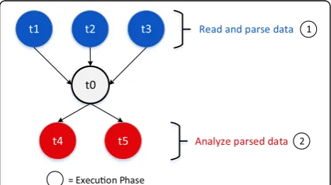
The system is subject to an open stream of multi-stage jobs. Each multi-stage jobj that arrives on the system is characterized by an earliest start time (sj) and an end-to-end deadline (dj) by which the jobjshould complete exe-cuting. In addition, each jobjalso comprises a set of tasks, where each taskthas an execution time (et) and can have one or more precedence relationships. The multi-stage job and the precedence relationships between its tasks can be modelled using a directed acyclic graph (DAG) (see Fig. 2, for example). The nodes (vertices) of the DAG rep-resent the tasks of the job, and the edges of the DAG show the precedence relationships between the tasks of the job.
start executing until task t0 finishes, which in turn cannot start executing until tasks t1, t2, and t3 finish executing. Note that some workflows are modelled using a DAG with special tasks, referred to as dummy tasks, whose only purpose is to enforce precedence relation-ships between tasks in the DAG, and thus, dummy tasks have an execution time equal to 0. For example, in Fig. 2, task t0 is a dummy task that ensures tasks in the second phase of execution start to execute only after all the tasks in the first phase have completed.
As shown in Fig. 1, jobs that arrive on the system are placed in a job queue, where jobs are sorted by non-decreasing order of their deadlines (i.e., jobs that have earlier deadlines are placed in front of jobs with later deadlines). The resource manager uses RM-DCWF, pre-sented in this paper, to perform matchmaking and sched-uling. More specifically, when the resource manager is available (i.e., not busy mapping another job) and the job queue is not empty, it removes the first job in the job queue to map onto the resources of the system,R. The re-quirements for mapping the jobs on to R are described
next. The tasks of each jobjcan only execute aftersjand after their parent tasks have completed executing. In addition, each task of jobjshould complete its execution before the deadline of the job (dj); otherwise, job j will miss its deadline. Note thatdjis a soft deadline, meaning that although jobs are permitted to miss their deadlines, the desired system objective is to minimize the number of late jobs. At any point in time, the number of tasks that a resource rin Rcan execute in parallel must be less than or equal to its capacity, cr. A resource will execute the tasks it has been assigned in the order generated by RM-DCWF. However, a task that has been scheduled but has not started executing can be rescheduled or assigned to another resource, if required.
Deadline budgeting algorithm for workflows Algorithm 1 presents the Deadline Budgeting Algorithm for Workflows (DBW algorithm), which is used by RM-DCWF to decompose the end-to-end deadline of a multi-stage job into components and to assign each task of the job a sub-deadline. The input required by the DBW algo-rithm is a multi-stage job j and two integer arguments: setOpt to indicate the approach used to calculate the sam-ple execution time of the jobj (SETj) and laxDistOpt to specify how thelaxity(orslack time) of the jobj(Lj) is to be distributed among its constituent tasks.SETjis an esti-mate of the execution time of job j that is calculated by the DBW algorithm andLjis the extra time that jobjhas for meeting its deadline, if it starts executing at its earliest start time.Ljis calculated as follows:
Lj¼dj−sj−SETj ð1Þ
The first step of the DBW algorithm is to calculate SETj(line 1).SETjis calculated using the user-estimated
task execution times of the job and can be calculated in one of two ways, depending on the supplied setOpt argument. The first approach (setOpt = 1) is to calculate the execution time of job j when it ex-ecutes at its maximum degree of parallelism on the set of resources R with m resources, while not con-sidering any contention for resources (denoted SETjR). Recall from the previous section, the definition of R, which is a set of resources that models the distrib-uted system job j will execute on. The approach used by the algorithm for matchmaking and scheduling the tasks of job j onto the m resources and computing SETjR is briefly described. The tasks of job j are allo-cated in non-increasing order of their execution times: the ready task with the highest required task execution time is allocated first; the task with the next highest execution time is considered next and so on. Tasks are considered ready when all of their par-ent tasks, as captured in the precedence graph that characterizes the workflow, have completed executing. A best-fit technique is used for allocating the tasks of the job to the resources. Each task of the job is allo-cated on that resource that can execute the task at its earliest possible time. Thus, the algorithm attempts to complete each task and the job at its earliest possible finish time. The second approach (setOpt = 2) is to calculate the execution time of the job when it exe-cutes on R, while considering the current processing load of the resources (i.e., considering the other jobs already executing or scheduled on R) (denoted SETjR_PL). This is accomplished by scheduling the job on the system’s resources to retrieve its expected completion time and then removing the job from the system. Next, the algorithm calculates the laxity of the job (Lj) using Eq. 1 (line 2). Note that when Lj is calculated using SETj equal to SETjR, the laxity of the job is referred to as the sample laxity (SL) because the job execution time is calculated on R without considering the current processing load of the re-sources in R. When Lj is calculated using SETj equal to SETj
R_PL
, the laxity of the job is referred to as thetrue laxity (TL) because the job execution time is calculated onRwhile considering the current processing load of the resources inR. The final steps of the algorithm are to dis-tribute the laxity of the job to each of its constituent tasks and to calculate a sub-deadline for each of the tasks (line 3) by invoking one of two algorithms devised: (1) the Pro-portional Distribution of Job Laxity (PD) Algorithm, which is described in Section "Proportional Distribution of Job Laxity Algorithm", and (2) the Even Distribution of Job Laxity (ED) Algorithm, which is discussed in Section "Even Distribution of Job Laxity Algorithm". The algorithm that is used depends on the supplied laxDistOpt input argument.
Proportional distribution of job laxity algorithm
The PD algorithm (shown in Algorithm 2) distributes the laxity of the job to its constituent tasks according to the length of the task’s execution time. This means that a task with a longer execution time is assigned a larger portion of the job’s laxity, resulting in the task having a higher sub-deadline. The input required by the algorithm in-cludes a job j to process and an integer argument, setOpt, to indicate how SETj is calculated. Recall from the discussion earlier thatSETjcan be calculated in one of two ways: setOpt = 1 corresponds to SETj
R and setOpt = 2 corresponds toSETjR_PL. A walkthrough of the algorithm is provided next.
The first step of Algorithm 2 is to calculate the sample completion time of jobj(denotedSCTj) as:
SCTj¼sjþSETj
where sj is the earliest start time of job j (line 1). The second and third steps involve retrievingsjandLj, respect-ively, of the supplied job j and saving them in local variables (lines 2–3). Next, the PD algorithm performs the following operations on each task t in the job j (line 4). The first operation is to calculate thecumulative laxityof the taskt(denotedCLt) (line 5) as:
CLt ¼
SCTt−sj
SCTj−sj
Lj
where SCTt is the sample completion time of task t. Note that the sample completion time of each task is determined during the calculation of SETj (line 1 in Algorithm 1) as follows:
SCTt¼stþet
wherestis the scheduled start time of taskt(determined by the scheduling algorithm) and etis the execution time of task t. The cumulative laxity of a task tis the maximum laxity that tasktcan have (i.e. the laxity that taskthas given that none oft’s preceding tasks, direct or indirect, use any of their laxities). After calculatingCLt, the sub-deadline of the taskt(sdt) is then calculated (line 6) as follows:
sdt ¼SCTtþCLt ð2Þ
method (lines 8–10). The objective of this method is to set the sub-deadline of all of t’s parent tasks to the sub-deadline of the task among all oft’s parent tasks that has the highest sub-deadline. The reason for performing this operation is that a tasktcannot start executing until all of its parent tasks finish executing, and thus, all the parent tasks of task tshould have the same sub-deadline. Note that after adjusting the sub-deadlines of the parents of task t, the sub-deadlines of the grandparents of tasktare not altered as they do not need to be adjusted. The PD algo-rithm ends after processing all the tasks in the jobj.
Even distribution of job laxity algorithm
The ED algorithm (see Algorithm 3) does not consider the length of the task’s execution time and instead distrib-utes the laxity of the job evenly among the execution phases of the job. Recall from Section "Problem Descrip-tion and Resource Management Model" that an execuDescrip-tion phase in a multi-stage job is a collection of tasks that perform a specific function in the job. The ED algorithm requires each task in a job to have an execution phase attribute, which is an integer (1, 2, 3,…) that indicates the phase of execution that the task belongs to. A walk-through of the ED algorithm is provided next.
The input required by the algorithm is a jobjto process. The first step is to retrieve the laxity of the job and save the value in a local variable (line 1). Next, the algorithm
retrieves the number of execution phases in jobjand stores the value in a variable named executionPhases (line 2). This is accomplished by checking the execution phase attribute of each tasktin jobj. The laxity that each execution phase should be assigned is then calculated as follows:
Lepj ¼Lj=nepj
where njep is the number of execution phases in job j (line 3). The cumulative laxity for each execution phase, which is the maximum amount of laxity that an execution phase can have, is then calculated as shown in lines 4–8. More specifically, the cumulative laxity of each execution phasephfor a jobjis calculated as:
CLphj ¼phLepj
wherephis an integer in the set {1, 2, 3,…,nj ep
} that rep-resents the execution phase. A map data structure named
cumulativeLaxitiesis used to store the cumulative laxity for each execution phase, where thekeyis the exe-cution phase and the value is the cumulative laxity. The last phase of the algorithm (lines 9–17) uses the cumula-tive laxity values to calculate and assign a sub-deadline for each of job j’s tasks. The following operations are per-formed on each tasktof jobj. First, the execution phase of the tasktis retrieved as shown in line 10. The cumula-tive laxity of the task is then retrieved from the cumulati-veLaxitiesmap using the value of the execution phase as the key (line 11). Next, the sub-deadline of the task is cal-culated using Eq.2and assigned to the task (lines 12–13). Similar to the PD algorithm, the ED algorithm invokes
setParentTasksSubDeadlines() if the task t has more than 1 parent task. After all the tasks of job jare processed the algorithm ends.
RM-DCWF’s matchmaking and scheduling algorithm This section describes RM-DCWF’s matchmaking and scheduling algorithm (also referred to as the mapping al-gorithm), which is composed of two sub-algorithms: (1) the Job Mapping algorithm (discussed in Section "Job Mapping Algorithm") and (2) the Job Remapping algo-rithm(described in Section "Job Remapping Algorithm"). When there is a job j available to be mapped, the Job Mapping algorithm is invoked. If the Job Mapping algo-rithm is unable to schedule jobjto meet its deadline, the Job Remapping algorithm is invoked to remap jobjand a set of jobs that may have caused jobjto miss its deadline.
Job mapping algorithm
instead of being local variables. A walkthrough of map-Job()is provided first, followed by a description of map-JobHelper(). The input required bymapJob()comprises the following: a job to mapj, an integersetOpt, an integer laxDistOpt, and an integer tsp. Note that except for the argument tsp, which specifies the task scheduling policy, these are the same input arguments used by the DBW algo-rithm. The method returns true if the jobjis scheduled to meet its deadline; otherwise, false is returned.
The first step ofmapJob()is to invoke the DBW algo-rithm to decompose the end-to-end deadline of the job j and assign each of jobj’s tasks a sub-deadline (line 1). Next, RM-DCWF’srootJobfield is set toj(line 2). The root-Job field stores the current job that is being mapped by RM-DCWF. The third step is to clear RM-DCWF’s pre-vRemapAttempts list (line 3), which stores the various sets of jobs that a job remapping attempt has previously processed. RM-DCWF’s jobComparator field, which specifies how jobs that need to be remapped are sorted, is then set to the Job Deadline Comparator (line 4) to sort jobs by non-decreasing order of their respective deadlines. A more detailed discussion of the purpose of these fields, which are used by the Job Remapping algorithm, is pro-vided in the next section. In line 5, RM-DCWF’s taskSchedulingPolicy field, which specifies how tasks are scheduled, is initialized. Two task scheduling pol-icies are devised.TSP1schedules tasks to execute at their earliest possible times, andTSP2schedules tasks to execute at their latest possible times such that the tasks meet their respective sub-deadlines. The last step is to invoke Al-gorithm 5:mapJobHelper()(line 6).
A walkthrough ofmapJobHelper(), which performs the allocation and scheduling of jobjonto the set of sources in the system, is provided next. The input re-quired by mapJobHelper() includes the following: a jobjto map, a BooleanisRootJob, which is set to true if this is the first time jobjis being mapped; otherwise, it is set to false, and a BooleancheckDeadline, which is set to true if the method should try to map job j to meet its deadline; otherwise, it is set to false and the method has to map jobjon the system, but it does not have to schedule job j to meet its deadline. The map-JobHelper() method starts by initializing the local variableisJobMapped to true (line 1). Next, all of job j’s tasks that need to be mapped are sorted in
non-increasing order of their respective execution times (line 2), where ties are broken in favour of the task with the earlier sub-deadline. If the tasks also have the same sub-deadline, the task with the smaller task id (a unique value) is placed ahead of the task with the larger id. The method then attempts to map each of jobj’s tasks (lines 3– 4) by performing the following operations for each tasktin jobj. First, the startTime variable is initialized by invoking the taskt’sgetEarliestStartTime()method (line 5), which returns the time that tasktcan start to execute while considering any precedence relationships that t has. If getEarliestStartTime() returns −1, it means that an earliest start time for tasktcannot be determined as yet because not all of taskt’s parent tasks have been scheduled. In this case,mapJobHelper()stops processing tasktfor the moment and attempts to map the next task in job j (line 6). On the other hand, if startTime is not−1, the pro-cessing of tasktcontinues. If RM-DCWF’s taskSchedu-lingPolicy field is set to TSP2 (line 7), the expected start time of the task is updated and set as shown in line 8. The expected completion time of the task is then calculated using the expected start time of the task (line 9).
After calculating the expected start time and completion time of taskt, the method checks whetherthas an execu-tion time equal to 0 (i.e., checks if tasktis a dummy task, defined in Section "Problem Description and Resource Management Model") (line 10). If tasktis a dummy task, it does not need to be scheduled on a resource because it has an execution time equal to 0 and only the task’s scheduled start time and completion time need to be set (line 11). The task t is also added to the RM-DCWF’s mapped-Tasks list (line 12), which stores all the tasks that have been successfully mapped for job j. On the other hand, if task thas an execution time greater than 0 (line 13), the method attempts to find a resourcerinRthat can execute tat its expected start time. Iftcannot be scheduled to exe-cute at its expected start time, the task is scheduled at the next best time depending on the value of the taskSche-dulingPolicy field (line 14). If taskScheduling-Policyis set to TSP1, the method schedules tasktat its next earliest possible time. On the other hand, if taskSchedulingPolicy is set to TSP2, the method schedules the task at its next latest possible time, while en-suring the task’s sub-deadline is satisfied.
(described in more detail in the next section) is then invoked and the return value is saved in a variable called isJob-Mapped(line 17). The next step (line 18) is then to go to line 27 to check the value of isJobMapped. If isJob-Mappedis set to true, meaning the job has been successfully scheduled to meet its deadline, the mappedTasks list is cleared, job j is added to RM-DCWF’s mappedJobs list (line 28), and true is returned (line 29). Otherwise, isJob-Mapped is set to false, meaning jobjcannot be scheduled to meet its deadline (line 30). This leads tomapJobHelper() being re-invoked, but this time with thecheckDeadline argument set to false, which will map jobjeven if it misses its deadline (line 31). False is then returned (line 32) to indi-cate jobjwill not meet its deadline.
If either of the conditions shown in line 15 are not true (i.e., a resource is found that can complete executing taskt before jobj’s deadline or the input argument checkDead-lineis false), it means that tasktcan be scheduled to exe-cute on resource r (line 20) and t is then added to the mappedTaskslist (line 21). The next task of jobjis then processed by repeating lines 3–26. This sequence of opera-tions continues until all of jobj’s tasks are mapped on the system. After all of job j’s tasks have been mapped, lines 27–29 are executed (as described earlier), and then the method returns.
Job remapping algorithm
The Job Remapping algorithm is comprised of two methods: (1)remapJob()presented in Algorithm 6 and (2)remapJobHelper()outlined in Algorithm 7. A dis-cussion of remapJob() is provided first, followed by a discussion on remapJobHelper(). The input argu-ments required byremapJob()include a jobjto remap and a BooleanisRootJob. TheisRootJobargument is set to true if it is the first invocation of remapJob() for attempting to remap jobjin this iteration; otherwise, isRootJobis set to false. If jobjand the set of jobs that may have prevented jobjfrom meeting its deadline are re-mapped and scheduled to meet their deadlines, the method returns true; otherwise, false is returned.
The first step of remapJob() is to set RM-DCWF’s taskSchedulingPolicyfield to TSP1 so the tasks that are remapped are scheduled to execute at their earliest pos-sible times (line 1). The second step is to invoke Algo-rithm 7:remapJobHelper()(line 2). Recall from line 4 of Algorithm 4 ((mapJob()) that the jobComparator field, which specifies how the jobs that need to be re-mapped are sorted, is initially set to theJob Deadline Com-parator. The Job Deadline Comparator sorts jobs in non-decreasing order of their respective deadlines with ties broken in favour of the job with the smaller laxity (i.e., tighter deadline). If remapJobHelper() returns true, remapJob() also returns true (line 3). On the other hand, if remapJobHelper() returns false, remap-Job() continues by checking the supplied isRootJob argument (line 4). IfisRootJobis false (line 5), meaning that this invocation of remapJob() is not for the ori-ginal attempt for mapping jobj, the method returns false to stop this particular remapping attempt from continuing (line 5). Otherwise, the method continues and RM-DCWF’s jobComparator field is changed to the Job Laxity Comparator (line 6) andremapJobHelper() is invoked again to check if remapping the jobs in a different order can generate a schedule in which all the jobs to re-map can meet their deadlines (line 7).
given priority. The normalized laxity of a jobj (denoted NLj) is calculated as follows:
NLj¼
Lj
SETj ð
3Þ
whereLjis the laxity of jobjandSETjis the sample execu-tion time of jobj(recall Section "Deadline Budgeting Al-gorithm for Workflows"). The reason for using NLj instead ofLjfor sorting the jobs is becauseLjis not always a good indicator of how stringent the deadline of a job is. A job can have a large laxity value, but still have a very tight deadline if the job has a high execution time. For ex-ample, given two jobs: (1) job j1 has sj1 equal to 0, dj1 equal to 6000, andSETj1equal to 5000, and (2) jobj2has
sj2 equal to 5500, dj2 equal to 6000, and SETj2 equal to 100. Using this information along with Eq. 1 and Eq. 3, the following values can be calculated:Lj1is equal to 1000,
Lj2is equal to 400,NLj1is equal to 0.2, andNLj2is equal to 4. As can be observed, job j1 has a higher laxity com-pared to jobj2(i.e.,Lj1>Lj2); however,j1’s normalized laxity is much smaller compared to j2’s normalized laxity (NLj1<NLj2), meaning jobj1has a more stringent deadline.
A walkthrough of remapJobHelper()(shown in Al-gorithm 7) is provided next. The input arguments and out-put value returned byremapJobHelper()are the same as those described forremapJob(). The first step of the method is to retrieve a subset of the jobs already scheduled on the system that may have caused jobjto miss its dead-line and store these jobs in thejobsToRemaplist (line 1). This includes all the jobs in RM-DCWF’smappedJobslist that execute within the interval [sj,dj]. Next, the supplied job j is added to the jobsToRemap list (line 2) and then the jobsToRemap list is sorted using RM-DCWF’s jobComparator(line 3). Since it is possible to have mul-tiple (nested) invocations ofremapJobHelper(), lines 4– 6 determine when an invocation of remapJobHelper() (referred to as a remapping attempt) should be rejected. More specifically, before a remapping attempt is started, the method checks if RM-DCWF’sprevRemapAttemptslist, which stores the various sets of jobs that previous invoca-tions ofremapJobHelper()have processed, contains the same jobs (in the same order) as thejobsToRemaplist (line 4). If this is true, the method returns false to stop the remap-ping attempt (line 5). On the other hand, if the remapremap-ping at-tempt is allowed to continue, the jobsToRemap list is added to RM-DCWF’s prevRemapAttempts list (line 7). Next, the method checks if the supplied argument isRootJobis true (line 8), and if so, the current state of the system is saved to a set of variables (line 9). This in-volves saving the scheduled tasks of each resource in the system and making a copy of RM-DCWF’smappedJobs list. Furthermore, the scheduled start time and assigned resource for each task currently mapped on the system is
saved. The reason for saving this information is because it may be changed during the job remapping attempt, and if the remapping attempt is not successful, the original state of the system has to be restored.
Time complexity analysis of the RM-DCWF matchmaking and scheduling algorithm
As discussed in this section, the worst-case time com-plexity of the RM-DCWF matchmaking and scheduling algorithm is O(n2) where n is the number of jobs (or workflows) that arrive on the system. In the worst-case scenario, the algorithm will have to reschedule all the jobs in the system each time a new job arrives. For ex-ample, given n = 100, we have the following scenario. First, a job j1 arrives on the system and is scheduled. Sometime later, a new jobj2(with a deadline that is earl-ier than j1’s deadline) arrives before jobj1 is completed and the algorithm schedules j2 and reschedules j1. Be-fore jobsj1andj2complete, a new jobj3with a deadline that is earlier than the deadlines ofj1and j2arrives. The algorithm schedules j3 and then reschedules j1 and j2. This process continues for the remaining 97 jobs that ar-rive on the system. The total number of jobs that the al-gorithm schedules in this worst case is then equal to:
1þ2þ3þ…þn¼n
ðnþ1Þ
2 ¼
n2þn 2
Thus, the worst-case time complexity of the algorithm is O(n2). Note that in practice, the time complexity of the al-gorithm will be lower because not all jobs will need to be rescheduled when a new job arrives on the system. For ex-ample, some jobs will have completed executing and other jobs will not need to be rescheduled because they do not contend with the same time slots as the newly arriving job. Moreover, if scheduling a job is deemed to take too long be-cause of the large number of jobs that need to be resched-uled, it is possible to limit the number of jobs to reschedule. For example, this can be accomplished by modifying line 1 of Algorithm 7 to restrict the size of the jobsToRemap list. Such a modification will limit the number of jobs that can be added to the list, thus limiting the number of jobs that can be rescheduled at a given point in time.
Furthermore, an in-depth and rigorous empirical per-formance evaluation of the algorithms using various workloads and workload and system parameters is pre-sented in Section "Performance Evaluation of RM-DCWF". The results of the performance evaluation (dis-cussed in more detail in Section "Results of the Factor-at-a-Time Experiments") demonstrate that the algorithm leads to a reasonably small system overhead. For ex-ample, in experiments with a very high contention for resources, leading to an average resource utilization of 0.9, the average matchmaking and scheduling time of the algorithm was measured to be less than 0.05 s.
Performance evaluation of RM-DCWF
This section describes the two types of simulation experiments conducted to evaluate the performance of
RM-DCWF. The first type of experiments (presented in Section "Results of the Factor-at-a-Time Experiments" and Section "Investigation of Using a Small Number of Re-sources") investigate the effect of various system and workload parameters on the performance of RM-DCWF. More specifically, factor-at-a-time experiments are con-ducted where one parameter is varied and the other pa-rameters are kept at their default values. The second type of experiments (presented in Section "Comparison with a First-in-first-out (FIFO) Scheduler" and Section "Compari-son with MCRP-RM") compare the performance of RM-DCWF with that of a FIFO Scheduler and the MapReduce Constraint Programming based Resource Management technique (MRCP-RM) described in [29], respectively. MRCP-RM has objectives that are similar to that of RM-DCWF: perform matchmaking and scheduling for an open stream of multi-stage jobs with SLAs, where each job’s SLA is characterized by an earliest start time, an exe-cution time, and an end-to-end deadline.
The rest of this section is organized as follows. The ex-perimental setup and the metrics used in the performance evaluation are described in Section "Experimental Setup". Following this, a description of the system and workload parameters used in the factor-at-a-time experiments is pro-vided in Section "System and Workload Parameters for the Factor-at-a-Time Experiments". The results of the experi-ments are then presented and discussed.
Experimental setup
The experiments are executed on a PC running Windows 10 (64-bit) with an Intel Core i5–4670 CPU (3.40 GHz) and 16 GB of RAM. Note that in the experiments, only the execution of the workload on the system is simulated. RM-DCWF and its associated algorithms are executed on the PC that was described at the beginning of this section. RM-DCWF is evaluated in terms of the following per-formance metrics in each simulation run:
Proportion of Late Jobs(P) =N/nwhereNis the number of late jobs in a simulation run andnis the total number of jobs processed during the simulation.
Average Job Turnaround Time(T). The turnaround
time of a jobj(tatj) isCTj–sjwhereCTjis jobj’s
completion time andsjisj’s earliest start time,
respectively. Thus,T=∑j∈J(tatj)/n.
Average Job Matchmaking and Scheduling Time(O)
is the average processing time required by RM-DCWF to partition a job’s deadline among its tasks and matchmake and schedule a job.O=∑j∈J(oj)/nwhere ojis the processing time required for mapping jobjon
the system.
produced as outputs of the simulation. TheO-by-T ratio (denoted O/T) is used as an indicator of the processing overhead of RM-DCWF. This is an appropriate indication of the processing overhead because it puts the measured values of the algorithm runtimes (O) into context by con-sidering the value of O relative to the mean job turn-around time (T).
System and workload parameters for the factor-at-a-time experiments
The workloads used in the factor-at-a-time experiments are based on real scientific applications (workflows) that have been described in the literature. More specif-ically, the three scientific applications that are used in the experiments are named CyberShake, LIGO, and Epigenomics. A brief discussion of each application that includes presenting the DAG of the workflow is pro-vided next. A more detailed description of all three applications can be found in [33].
CyberShake is a seismology application that is created by the Southern California Earthquake Center to predict earth-quake hazards in a region. The DAG of a sample Cyber-Shake workflow is presented in Fig. 3. As shown, the workflow has five phases of execution. Recall from Section "Problem Description and Resource Management Model" that the numberiin the small circle indicates theith execu-tion phase. The first, second, and fourth execuexecu-tion phases each contain multiple tasks to execute whereas the third and fifth execution phase each only have one task to execute.
The Laser Interferometer Gravitational Wave Observatory (LIGO) Inspiral Analysis workflow is used to search for and analyze gravitational waveforms in data collected by large-scale interferometers. The input data is parti-tioned into multiple blocks so that the data can be ana-lyzed in parallel. Fig. 4 shows the DAG of a sample LIGO workflow, which has 6 phases of execution. In this
sample LIGO workflow there are two blocks of data be-ing processed in parallel, where each block of data has multiple waveform data (i.e. TmptlBank tasks) to process.
The Epigenomics (Genome) workflow is used for auto-mating several commonly used operations in genome se-quence processing. Fig. 5 shows a DAG of a sample Genome workflow, which is characterized by one or morelanes, each of which starts with the execution of a fastQSplit task. If there is more than one lane in the workflow, as shown in the example in Fig. 5, there are two mapMerge stages. The first mapMerge stage is for merging the results within a particular lane (execution phase 6), and the second mapMerge stage (referred to as the global mapMerge stage) is for merging the results of all the lanes in the workflow (execution phase 7).
Table 1 outlines the system and workload parameters used in the factor-at-a-time experiments. These experi-ments investigate the effect of the following parameters on system performance: job arrival rate, earliest start time of jobs, job deadlines, and the number of resources. A walkthrough of Table 1 is provided next. Note that the distributions used to generate the parameters of the work-load, including the job arrival rate, earliest start time of jobs, and job deadlines are adopted from [11, 29]. The first component of the table describes the workload. For a given workflow type (CyberShake, LIGO, or Genome), there are three job sizes, each of which has an equal prob-ability of being submitted to the system: small, medium, andlarge, comprising 30 tasks, 50 tasks, and 100 tasks, re-spectively. The distributions used for generating the exe-cution times of the tasks for each workload are described in [33]. The open stream of job arrivals is generated using a Poisson process. The arrival rates used in the experi-ments of a given workload type are different since each of the workloads is characterized by jobs with different exe-cution times. The average exeexe-cution time of a CyberShake
job, LIGO job, and Genome job on a single resource is equal to 1551 s, 13,300 s, and 160,213 s, respectively. The parametersλCS,λLG, andλGNspecify the job arrival rates used for the CyberShake, LIGO, and Genome workloads, respectively. The arrival rates for each workflow are chosen such that resource utilization ranging from moder-ate (~50%) to modermoder-ately-high (~70%) to high (~90%) is generated on the system when using the default number
of resources (50 resources, where each resource has a cap-acity equal to 2). The earliest start time of a jobj(sj) can be its arrival time (atj) or at a time in the future afteratj. A random variable x, which follows a Bernoulli distribu-tion with parameterp, is defined. The parameter pis the probability that a job jhassj greater thanatj. Ifxis 0, sj equalsatj; otherwise,sjequals the sum ofatjand a value generated from a discrete uniform (DU) distribution with a lower-bound equal to 1 and an upper-bound equal to a parametersmax. The deadlines of the jobs are generated by multiplyingSETj
R
(recall Section "Deadline Budgeting Al-gorithm for Workflows") with anexecution time multiplier (em) and adding the resulting value tosj. The parameter emis used to determine the laxity (or slack time) of a job and is generated using a uniform distribution (U) where 1 is the lower-bound and emmaxis the upper-bound of the distribution.
The remaining components of Table 1 describe the sys-tem used to execute the jobs and the configuration of RM-DCWF. The number of resources (m), which repre-sents the number of nodes in the distributed system for processing the jobs, is varied from 40 to 50 to 60, where each resource has a capacity (cr) equal to 2. Recall from Section "Problem Description and Resource Management Model",crspecifies the number of tasks that a resourcer can execute in parallel at any given point in time. RM-DCWF’s Job Mapping algorithm can handle resources with different values of cr as the algorithm performs re-source allocation and scheduling by considering the set of all the resource slots provided by all the resources in R. Note that how the capacity of the resources, as reflected by their number of resource slots, is distributed among the individual resources in the system does not affect performance because matchmaking and scheduling are performed on the resource slots, each of which has an equal speed of execution. As a result, system performance does not change ifcris different for the different resources inRas long as the sum of the number of resource slots in all the resources in R remains the same. Thus, the total resource capacityof the system, the sum of the number of resource slots for all the resources in R, is an important parameter that can affect system performance. This par-ameter is varied by varying the value ofmin the experi-ments described in Section "Effect of the Number of Resources".
The configuration of RM-DCWF is defined as x-y-z where x specifies the laxity distribution algorithm (i.e., PD or ED, described in Section "Deadline Budgeting Al-gorithm for Workflows"), y specifies the approach to calculate the laxity of the job (i.e., SL or TL, described in Section "Deadline Budgeting Algorithm for Work-flows"), and z specifies the task scheduling policy (i.e., TSP1 or TSP2, described in Section "Job Mapping Al-gorithm"). In total, there are 8 different RM-DCWF
Fig. 4DAG of a sample LIGO application (based on [33])
configurations, and thus, for each workload type, the factor-at-a-time experiments are conducted 8 times. This is performed to determine which configuration provides the best performance for a given workload.
Results of the factor-at-a-time experiments
The results of the factor-at-a-time experiments are pre-sented in this section. Each simulation run was executed long enough to ensure that the system was operating at a steady state. Furthermore, each factor-at-a-time experi-ment is repeated a sufficient number of times such that the desired trade-off between simulation run length and accuracy of results was achieved. The confidence inter-vals for T and O at a confidence level of 95% are ob-served to remain less than ±5% of the respective average values in most cases. For P, the confidence intervals are observed to be in most cases less than ±10% of the aver-age value. Such an accuracy of the simulation results is deemed adequate for the nature of the investigation: the focus of which is investigating the trend in the variation of a given performance metric in response to changes in the system and workload parameters and to compare the performance of the various RM-DCWF configura-tions. The values averaged over the simulation runs and the confidence intervals are shown in the figures and ta-bles presented in this section. In the figures, the confi-dence intervals are shown as bars originating from the mean values; however, some of the bars are difficult to see since the confidence intervals are small. Note that the confidence intervals are considered while deriving a conclusion regarding the relative performance of the re-spective RM-DCWF configurations.
To conserve space and provide clarity of presentation, only the results of the two RM-DCWF configurations, one using PD and the other one using ED, that demon-strated the best overall performance in terms of P are presented in the following sub-sections. A more detailed discussion of the results of the performance evaluation can be found in [34]. More specifically, the two RM-DCWF configurations that are compared for each work-load type are summarized:
PD-SL-TSP1 vs ED-SL-TSP2 for the CyberShake workload
PD-SL-TSP1 vs ED-SL-TSP1 for the LIGO workload PD-SL-TSP1 vs ED-SL-TSP1 for the Genome
workload
Note that in the following sub-sections, the results of the experiments using the CyberShake workload are shown in figures, wherePis displayed in its own figure and T and O are graphed in the same figure with T being displayed as a bar graph that uses the scale on the left Y-axis and O being displayed as a sequence of points that uses the scale on the right Y-axis. To main-tain a reasonable number of figures, the results of each of the experiments using the LIGO and Genome work-loads are shown in their own tables where the values of P,T, andOcan be presented concisely.
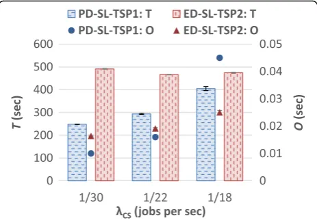
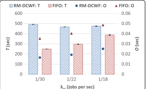
Effect of job arrival rate
The impact of the job arrival rate on system perform-ance is discussed in this section. The results of the experiments using the CyberShake workload are
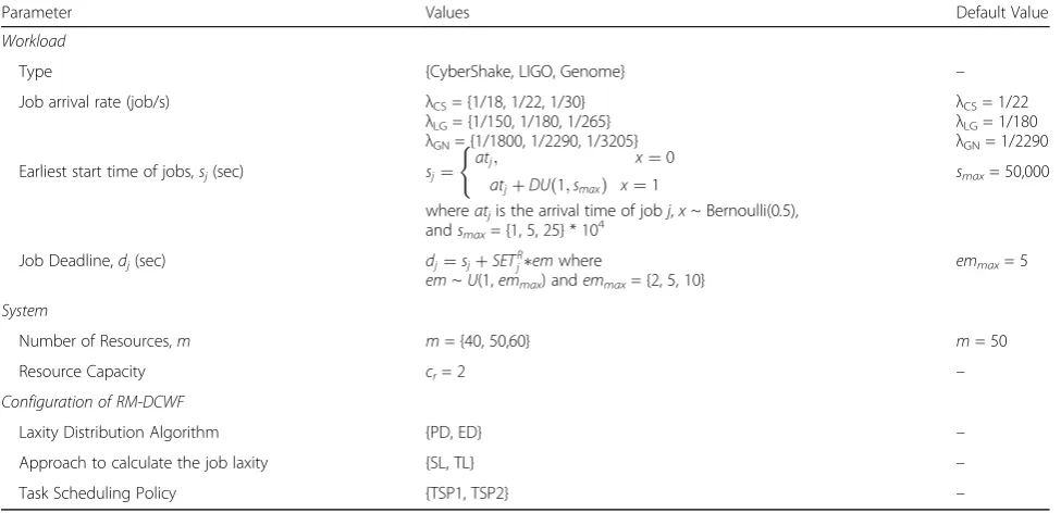
Table 1System and Workload Parameters for the Factor-at-a-Time Experiments
Parameter Values Default Value
Workload
Type {CyberShake, LIGO, Genome} –
Job arrival rate (job/s) λCS= {1/18, 1/22, 1/30}
λLG= {1/150, 1/180, 1/265}
λGN= {1/1800, 1/2290, 1/3205}
λCS= 1/22
λLG= 1/180
λGN= 1/2290
Earliest start time of jobs,sj(sec) sj¼
atj; x¼0
atjþDUð1;smaxÞ x¼1 (
whereatjis the arrival time of jobj,x~ Bernoulli(0.5), andsmax= {1, 5, 25} * 104
smax= 50,000
Job Deadline,dj(sec) dj¼sjþSETRjemwhere
em~U(1,emmax) andemmax= {2, 5, 10}
emmax= 5
System
Number of Resources,m m= {40, 50,60} m= 50
Resource Capacity cr= 2 –
Configuration of RM-DCWF
Laxity Distribution Algorithm {PD, ED} –
Approach to calculate the job laxity {SL, TL} –
presented in Fig. 6 and Fig. 7. The figures show that for PD-SL-TSP1, P,T, and O increase with λCS. When λCS is high, jobs arrive on the system at a faster rate, which leads to more jobs being present in the system at a given point in time and an increased contention for re-sources. This in turn prevents some jobs from execut-ing at their earliest start times, resultexecut-ing inTincreasing and some jobs to miss their deadlines (which increases P). The increased contention for resources also causes O to increase because RM-DCWF takes more time to find a resource to map the tasks of the job such that the job does not miss its deadline. Furthermore, since jobs are more prone to miss their deadlines at high values of λCS, RM-DCWF’s Job Remapping algorithm, which is a source of overhead, is invoked more often, contributing to the increase inO.
It is observed that for ED-SL-TSP2,P and Oincrease with λCS, and T tends to remain relatively stable. In addition, when λCS is 1/22 jobs per sec or lower, both systems achieve comparable values ofP; however, when
λCS is 1/18 jobs per sec, ED-SL-TSP2 is observed to achieve a lowerP. This can be attributed to ED-SL-TSP2 efficiently using the laxity of jobs to delay the execution of jobs with a later deadline to execute jobs with an earlier deadline, which in turn reduces the contention for resources at certain points in time and leads to a lower P. Although, as shown in Fig. 7, by delaying the execution of jobs, ED-SL-TSP2 achieves a higher T compared to PD-SL-TSP1. The O of ED-SL-TSP2 is higher compared to that of PD-SL-TSP1 whenλCSis 1/ 22 jobs per sec or smaller. This is because more time is required by TSP2 to search for a resource that can exe-cute a task at its latest possible time such that its sub-deadline is satisfied, compared to the time required by TSP1 to find a resource to execute tasks at their earliest possible times. However, whenλCS is 1/18 jobs per sec,
PD-SL-TSP1 has a higherO, which can be attributed to the Job Remapping algorithm being invoked more often when using PD-SL-TSP1 compared to when using ED-SL-TSP2.
Table 2 and Table 3 present the results of the experi-ments when using the LIGO workload and the Genome workload, respectively. Unlike the CyberShake work-load, when using the LIGO and Genome workloads, configuring RM-DCWF to use ED with TSP2 did not produce a better performance in comparison to using ED with TSP1. This demonstrates that TSP2 is only ef-fective for certain workflows and the average job execu-tion time and the structure of the job (e.g., precedence relationships between the tasks of the job) can affect the performance of TSP2. As shown in the tables, the trend in performance ofP,T, andOare identical to that of the CyberShake workload when using PD-SL-TSP1. Furthermore, the results also show that both PD-SL-TSP1 and ED-SL-PD-SL-TSP1 achieve very similar results be-cause TSP1 schedules tasks to start executing at their earliest possible times, regardless of their respective sub-deadlines. Over all the experiments performed to investigate the effect of the job arrival rate, the results demonstrate that RM-DCWF can achieve low values of P(less than 2% even at high arrival rates) and has a low
Fig. 6Effect ofλCSonPwhen using the CyberShake workload
Fig. 7Effect ofλCSonTandOwhen using the CyberShake workload
Table 2LIGO workload: effect ofλLGonP,T, andO
λLG(jobs/s) P (%) T (sec) O (sec)
PD-SL-TSP1
ED-SL-TSP1
PD-SL-TSP1
ED-SL-TSP1
PD-SL-TSP1
ED-SL-TSP1 1/265 0.02 0.02 1346 1346 0.008 0.008
±0.01 ±0.01 ±0.6 ±0.6 ±0.00 ±0.00
1/180 0.11 0.11 1466 1466 0.009 0.009
±0.01 ±0.01 ±4.6 ±4.6 ±0.00 ±0.00
1/150 1.03 1.06 2005 2006 0.017 0.016
processing overhead as indicated by the small O (less than 0.025 s) and smallO/T(less than 0.005%).
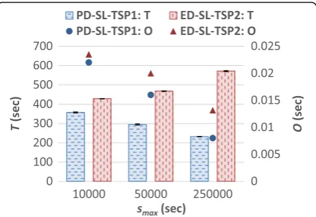
Effect of earliest start time of jobs
The impact of the earliest start time of jobs on system performance is described in this section. Fig. 8 and Fig. 9 present the results when using the CyberShake work-load. It is observed that for PD-SL-TSP1,P,T, and O de-crease with an inde-crease insmax. Whensmax is large, jobs have a wider range of earliest start times with some jobs having an earliest start time near their arrival times, while other jobs have their earliest start times further in the future. This leads to less contention for resources and allows more jobs to execute at or closer to their earliest start times, resulting in a lowerP,T,andO. Simi-lar to PD-SL-TSP1, it is observed that for ED-SL-TSP2, P and O decrease as smax increases. However,T is ob-served to increase withsmax. This is due to ED-SL-TSP2 scheduling tasks to execute at their latest possible times, while ensuring the respective sub-deadlines of the tasks are met. When the contention for resources is low (e.g., when smax is large), ED-SL-TSP2 can more readily schedule tasks to start executing at their latest possible start times since jobs are less prone to miss their dead-lines and the Job Remapping algorithm does not need to
be invoked as often. Overall, it is observed that similar to the results presented in the previous section, ED-SL-TSP2 tends to achieve a lowerP(35% lower on average), but this is accompanied by a higher T (75% higher on average) and higher O (32% higher on average) com-pared to PD-SL-TSP1.
The results of the experiments using the LIGO work-load are presented in Table 4. It is observed that for both systems,P,T, andOseem to be insensitive tosmax, which is different from the results of PD-SL-TSP1 shown in Fig. 8 and Fig. 9, where P, T, and O are observed to decrease assmaxincreases. The reason for this can be at-tributed to the LIGO workload comprising jobs with higher average execution times compared to those of the CyberShake workload, as well as the values ofsmax used not significantly reducing the amount of jobs that have overlapping execution times (i.e., not reducing the con-tention for resources). The average job execution time (on a single resource) of the CyberShake workload (equal to 1551 s) is much smaller compared to that of the LIGO workload (13,300 s).
Table 5 presents the results of the experiments using the Genome workload. It is observed that P and T tend to increase and O remains stable as smax increases. The increase in P could be attributed to the values of smax experimented with (e.g., 50,000 and 250,000 s) causing more jobs to have overlapping execution times and thus increasing the contention for resources. This did not hap-pen when using the other two workloads because the Genome workload comprises jobs with very high average execution times (~160,213 s on a single resource), which is significantly higher compared to those of the Cyber-Shake and LIGO workloads. Increasing the values ofsmax experimented with when using the Genome workload is expected to generate a similar trend in performance to the results of the CyberShake workload. This is because there will be less chance for the execution of jobs to overlap with one another.
Table 3Genome workload: effect ofλGNonP,T, andO
λGN(jobs/s) P (%) T (sec) O (sec)
PD-SL-TSP1
ED-SL-TSP1
PD-SL-TSP1
ED-SL-TSP1
PD-SL-TSP1
ED-SL-TSP1
1/3205 0.01 0.01 17,544 17,544 0.008 0.008
±0.00 ±0.00 ±927 ±927 ±0.000 ±0.000
1/2290 0.07 0.07 17,963 17,963 0.008 0.008
±0.01 ±0.01 ±1007 ±1007 ±0.000 ±0.000
1/1800 1.43 1.40 52,312 52,472 0.048 0.051
±0.45 ±0.44 ±12,915 ±13,003 ±0.015 ±0.016
Fig. 8Effect ofsmaxonPwhen using the CyberShake workload
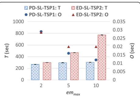
Effect of job deadlines
The impact of job deadlines on system performance is presented in this section. The results of the experiments using the CyberShake workload, as depicted in Fig. 10 and Fig. 11, show that for both systems, P decreases as emmax increases. This is because at a higheremmax jobs have more laxity and are thus less susceptible to miss their deadlines. Moreover, for ED-SL-TSP2, T is ob-served to increase asemmaxincreases. This can be attrib-uted to jobs not having to execute at or close to their sj to meet their deadlines when they have more slack time and the Job Remapping algorithm having to be executed less often. In addition, RM-DCWF may delay the execu-tion of some jobs to allow a job with an earlier deadline to execute first. On the other hand, whenemmaxis small, jobs need to execute closer to their earliest start times and the Job Remapping algorithm is invoked when a job cannot be scheduled to meet its deadline. Ois thus ob-served to increase for both systems, as emmax decreases because it leads to multiple invocations of the Job Remap-ping algorithm.
When comparing PD-SL-TSP1 and ED-SL-TSP2, it is observed that both systems perform comparably in terms ofPwhenemmaxis 5 or 10. However, whenemmax is 2, it is observed that PD-SL-TSP1 achieves a smallerP compared to ED-SL-TSP2. This is because when the deadlines of the jobs are more stringent, jobs need to execute closer to their earliest start times to meet their deadlines, which agrees with the objective of TSP1 and not with the objective of TSP2, which schedules jobs to
execute at their latest possible times. Similar to the re-sults described in the previous sections, PD-SL-TSP1 also achieves a lower Tand a lower or similar O com-pared to ED-SL-TSP2.
The results of the experiments using the LIGO work-load and Genome workwork-load are presented in Table 6 and Table 7, respectively. It is observed that the trend in per-formance observed for both systems when using the LIGO and Genome workloads are identical to that of the Cyber-Shake workload when using PD-SL-TSP1:P decreases,O decreases, andTremains approximately at the same level as emmax increases. Overall, it is observed that RM-DCWF can achieve a low P (less than 4.2%) even when jobs have tight deadlines (i.e.,emmaxis 2). In addition,Ois small (less than 0.03 s), and the processing overhead, as indicated byO/T,is less than 0.01% for all the experiments described in this sub-section.
Table 5Genome workload: effect ofsmaxonP,T, andO
smax(sec) P (%) T (sec) O (sec)
PD-SL-TSP1
ED-SL-TSP1
PD-SL-TSP1
ED-SL-TSP1
PD-SL-TSP1
ED-SL-TSP1
10,000 0.04 0.04 17,693 17,693 0.008 0.008
±0.01 ±0.01 ±959 ±959 ±0.000 ±0.000
50,000 0.07 0.07 17,963 17,963 0.008 0.008
±0.01 ±0.01 ±1007 ±1007 ±0.000 ±0.000
250,000 0.08 0.08 18,171 18,171 0.008 0.008
±0.01 ±0.02 ±1049 ±1049 ±0.000 ±0.000
Fig. 10Effect ofemmaxonPwhen using the CyberShake workload
Fig. 11Effect ofemmaxonTand Owhen using the CyberShake workload
Table 4LIGO workload: effect ofsmaxonP,T, andO
smax(sec) P (%) T (sec) O (sec)
PD-SL-TSP1
ED-SL-TSP1
PD-SL-TSP1
ED-SL-TSP1
PD-SL-TSP1
ED-SL-TSP1
10,000 0.10 0.10 1450 1450 0.009 0.009
±0.01 ±0.01 ±3.3 ±3.3 ±0.000 ±0.000
50,000 0.11 0.11 1466 1466 0.009 0.009
±0.01 ±0.01 ±4.6 ±4.6 ±0.000 ±0.000
250,000 0.09 0.08 1441 1427 0.009 0.009
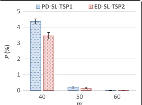
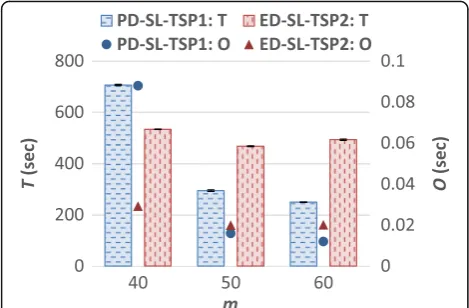
Effect of the number of resources
In this section, the impact of m, the number of re-sources, on system performance is discussed. From the results of the experiments using the CyberShake work-load (refer to Fig. 12 and Fig. 13), it is observed that for PD-SL-TSP1, P, T, andO decrease asm increases. This is because as m increases, there are more resources in the system to execute the jobs, leading to a lower con-tention for resources. The reason for the higher O when m is small can be attributed to the Job Mapping algorithm requiring more time to find a resource to map a task. When there are fewer resources in the sys-tem (smallm), there are more tasks scheduled on each resource, leading to more time being required to find the ideal resource to execute a task. In addition, the high contention for resources makes jobs susceptible to miss their deadlines and leads to RM-DCWF’s Job Remapping algorithm being invoked more often.
For ED-SL-TSP2,P, T, and Ofollow a similar trend in performance as observed for PD-TL-TSP1, except when mis 60. Whenmis 60,Tis slightly higher compared to the case when m is 50. This can be attributed to the availability of ten additional resources, resulting in a lower contention for resources and a smallerP, and thus leading to a lower number of invocations of the Job Remapping Algorithm, which remaps jobs to start exe-cuting at their earliest possible times. This in turn allows TSP2 to schedule more tasks to execute at their latest possible times, while satisfying their respective sub-deadlines.
When comparing the performance of PD-SL-TSP1 and ED-SL-TSP2 for the CyberShake workload, it is ob-served that ED-SL-TSP2 achieves a smaller P and the most significant reduction in P is observed when m is 40 (refer to Fig. 12). Similar to the results presented in the previous sections (see Fig. 6, for example), schedul-ing tasks to execute at their latest possible time, while satisfying their respective sub-deadlines (i.e., using TSP2) tends to give rise to a lower P but a higher T when processing the CyberShake workload. The lower Pcan be attributed to ED-SL-TSP2 efficiently using the laxity of jobs to delay the execution of jobs with a later
deadline to execute those with an earlier deadline. However, as shown in Fig. 13, it is observed that when m is 40, PD-SL-TSP1 achieves a higher Tcompared to ED-SL-TSP2. This can be attributed to PD-SL-TSP1 delaying the execution of multiple jobs that miss their deadlines for a long period of time for executing jobs that have not missed their deadlines. In the case of ED-SL-TSP2, fewer jobs need to be delayed because when mis 40, ED-SL-TSP2 achieves a smallerPcompared to PD-SL-TSP1 (refer to Fig. 12).
The results of the experiments using the LIGO work-load (see Table 8) and the Genome workwork-load (see Table 9) follow a similar trend in system performance to that of the CyberShake workload when using PD-SL-TSP1:P decreases,T decreases, and Otends to decrease asmincreases. It is observed once again that both PD-SL-TSP1 and ED-SL-PD-SL-TSP1 achieve similar results for both workloads. When m is 60, O is observed to be slightly higher compared to when mis 50. Even though, there is less contention for resources whenmis 60, the Job Map-ping algorithm may need to search through more re-sources to find the resource to schedule a task to start at its earliest possible time. This in turn leads to a slight in-crease inO.
Table 6LIGO workload: effect ofemmaxonP,T, andO
emmax P (%) T (sec) O (sec)
PD-S-TSP1
ED-SL-TSP1
PD-SL-TSP1
ED-SL-TSP1
PD-SL-TSP1
ED-SL-TSP1
2 2.44 2.43 1458 1457 0.012 0.011
±0.14 ±0.14 ±4.4 ±4.4 ±0.000 ±0.000
5 0.11 0.11 1466 1466 0.009 0.009
±0.01 ±0.01 ±4.6 ±4.6 ±0.000 ±0.000
10 0.04 0.04 1458 1463 0.009 0.008
±0.01 ±0.01 ±6.2 ±4.6 ±0.000 ±0.000
Table 7Genome workload: effect ofemmaxonP,T, andO
emmax P (%) T (sec) O (sec)
PD-SL-TSP1
ED-SL-TSP1
PD-SL-TSP1
ED-SL-TSP1
PD-SL-TSP1
ED-SL-TSP1
2 0.49 0.49 17,933 17,933 0.009 0.009
±0.12 ±0.12 ±1001 ±1001 ±0.000 ±0.000
5 0.07 0.07 17,963 17,963 0.008 0.008
±0.01 ±0.01 ±1007 ±1007 ±0.000 ±0.000
10 0.03 0.03 17,963 17,963 0.007 0.007
±0.01 ±0.01 ±1007 ±1007 ±0.000 ±0.000
![Fig. 3 DAG of a sample CyberShake application (based on [33])](https://thumb-us.123doks.com/thumbv2/123dok_us/850458.1582702/12.595.58.545.550.718/fig-dag-sample-cybershake-application-based.webp)
![Fig. 5 DAG of a sample Genome application (based on [33])](https://thumb-us.123doks.com/thumbv2/123dok_us/850458.1582702/13.595.56.291.87.305/fig-dag-sample-genome-application-based.webp)