AN EVALUATION OF SECURE ROUTING PROTOCOLS FOR MOBILE ADHOC NETWORKS

(1)

Chauhan. World Journal of Engineering Research and Technology

AN EVALUATION OF SECURE ROUTING PROTOCOLS FOR MOBILE

ADHOC NETWORKS

Alka Chauhan*

M.Tech Scholar, Department of Computer Science Engineering, Sachdeva Institute of Technology, Mathura, India. Dr. A. P. J. AKTU, Lucknow, India.

Article Received on 15/11/2017 Article Revised on 06/12/2017 Article Accepted on 27/12/2017

ABSTRACT

This paper presents Secure Routing Protocol (SRP), a new Routing strategy designed to improve load balancing and scalability in mobile ad hoc networks. SRP is a hop-by-hop routing protocol, which introduces flow-aware route discovery strategy to reduce the number of control overheads propagating through the network and distributes the flow of data through leastcon-gestednodes to balance the network traffic. SRP was implemented in Glomosim and compared with

AODV. To investigate the load distribution capability of FARP new performance metrics were introduced to measure the data packet flow distribution capability of the each routing protocol. The simulation results obtained illustrate that SRP achieves high levels of through - put, reduces the level of control overheads during route discovery and distributes the network load more evenly between nodes when compared to AODV. This paper also describes a number of Alter -native strategies and Improvements for the SRP.

KEYWORDS: Following the success of 2nd generation mobile (cellular) telephones.

INTRODUCTION

Following the success of 2nd generation mobile (cellular) telephones in the late 1990’s, the demand for wireless communication has continued to grow. Part of this success has been due to the growing demand in Internet type application over the wireless medium. This demand has partly been addressed through the introduction of 2.5G GPRS and more recently the 3G wjert, 2018, Vol. 4, Issue 1, 349-367.

World Journal of Engineering Research and Technology

WJERT

www.wjert.org

ISSN 2454-695X Original Article

SJIF Impact Factor: 4.326

*Corresponding Author Alka Chauhan

M.Tech Scholar, Department

of Computer Science

Engineering, Sachdeva

Institute of Technology,

Mathura, India. Dr. A.P.J.

(2)

(WCDMA1x) networks. Other solutions becoming widely popular are Wireless Local Area Networks (also known as Wi-Fi Hotspots), such networks are designed to extend the cover-age of wired networks by providing network access to mobile users. One shortcoming of the above technologies is their in-ability to provide a networking solution in environments where a networking infrastructure does not exists. Currently, infrastructured networks such as 2.5G, 3G and Wi-Fi Hotspots exist mainly in metropolitan areas, where consumer demand is high. To address this shortcoming a networking technology is required, which can be easily and cost effectively be configured without the need for a pre-existing infrastructure. One such solution is Ad hoc networking. In Ad hoc networks each end-user node is capable of sending, receiving and routing data packets in a distributed manner. Moreover, such networks can be con-figured to allow for mobility and perform routing over multiple hops. Such networks are commonly reffered to as Mobile Ad hoc Networks (or MANETs).

MANETs are still in their early development stage with the current areas of research spanning across all the levels of the traditional TCP/IP networking model. One interesting area of research in such networks is routing. Designing an efficient routing protocol for MANETs is a non-trivial task. This is primarily due to the dynamic nature of these networks, which requires intelligent strategies that can determine routes with minimum amount of overheads to ensure high levels of scalability. Consequently, researchers have proposed many different types of routing protocols for MANETs. These protocols can be categorised into three groups: proactive, reactive and hybrid routing. Proactive routing was the first attempt at designing routing protocols for MANETs. The early generation proactive protocols such as DSDV and GSR were based on the traditional distance vector and link state algorithm, which were originally proposed for wired networks. These protocols periodically maintain routes to all nodes with in the network the disadvantage of these strategies were the lack of their scalability due to exceedingly large amount of overhead they produced. More recent attempts at reducing control overhead in proactive routing can be seen in protocols such as OLSR.[8] and TBRPF.[3]

(3)

propagation of Route Request (RREQ) packets through the network. The second phase is initiated when a RREQ packet reaches a node, which has a route to the destination or the destination itself, in which case a Route Reply (RREP) packet is generated and transimited back to the source node. Reactive routing protocols produce significantly lower amount of routing overhead when compared proactive routing protocols when the number of flows in the network are low. However, for large number of flows reactive protocols experience a significant drop in data throughput. This is because routing control packets are usually flooded (globally) throughout the entire network to find a route to the destination. To reduce the global flooding in the network a number of different strategies have been proposed. In LAR and RDMAR the protocols attempt to use prior location knowledge of the destination to reduce the search zone during route discovery. In LPAR a combination of prior location knowledge and unicasting is used to reduce the number of rebroadcasting nodes within a search zone. In AODV the source nodes use Expanding Ring Search (ERS) to search nearby nodes first There-fore reducing the number of globally propagating control packets.

Hybrid routing protocols combine both reactive and proactive routing characteristics to achieve high levels of scalability. Generally in hybrid routing protocols, proactive routing is used within a limited region. These regions can be a cluster, a tree or a zone, which may contain a number of end-user nodes. Reactive routing is used to determine routes, which do not lie within a source node’s local region. The idea behind this approach to routing is to allow nearby nodes to collaborate and reduce the number of re-broadcasting nodes. Therefore, during a route discovery only a selected group of nodes within the entire network may rebroadcast packets.

While a great deal of attention has been paid to reducing routing overhead, not much attention has been paid in ensuring a fair distribution of traffic flow (or load) between the nodes. Most routing protocols proposed for MANETs select routes based on the shortest-path which is determined using hop count as the route selection metric. This can lead to congestion or the creation of traffic bottlenecks in the network, which can result s in higher levels of packets being dropped in the network and rapid depletion of resources in specific nodes.

(4)

a single route. In, a combination of a delay metric and hop count is used to select routes during the route discovery phase.

In this paper, we propose Flow-Aware Routing Protocol (FARP), a routing strategy which aims to reduce the amount of control overhead while ensuring a better distribution of traffic between the nodes. In FARP, a utility metric is introduced to restrict the propagation of Route Request (RREQ) packet over nodes with minimum number of active data flows from different source nodes Therefore, reducing congestion or the creation of bottleneck nodes. The rest of this paper is organised as follows. In section II, we present describe FARP section III describes the simulation environment, parameters and metrics used to investigate the performance of FARP with a number of routing protocols. Section IV presents a discussion for our simulation results. Section V presents a number of alternative strategies and improvements for FARP and section VI presents the conclusions of our paper.

II. Flow-Aware Routing Protocol

FARP employs the hop-by-hop routing strategy used in AODV. However, unlike AODV, FARP attempts to reduce the amount of control overhead while ensuring a better distribution of data traffic. This is achieved by introducing a flow-aware route discovery strategy, which select the nodes with the least number of traffic flows.

(5)

Algorithm FA

(∗The Flow-Add Algorithm ∗) 1. F lowt ← Flow expiration time

2. Flow ID ← Flow ID for the data packet 3. F lowT ← The flow table

4. F lowc ← Flow counter 5. F lowA ← Flow Update Flag 6. SID ← Source node ID 7. D ID ← Destination node ID

8. BID ← Previous forwarding node ID 9. Flow ID = SID|B ID|D ID

10.F ound ← F alse A flag used to fi nd Flow ID 11.for i ← 0, i < F lowc, i + +

12.if F lowT [i ].Flow ID = Flow ID 13.F ound ← T rue

14.break

15.if F ound = T rue 16.Set(F lowT [i ].F lowt) 17.else

18.F lowT [i ].Flow ID ← Flow ID 19.F lowT [i ].BID ← BID

20.Set(F lowT [i + 1].F lowt) 21.F lowc + +

22.if F lowc≥1 & F lowA! = Active 23.F lowA ← Active

24.Activate the Flow-Delete-Proactive function

(6)

The following algorithms illustrate the proactive (FDP) and Flow-Delete-reactive (FDR) strategies re-spectively.

Algorithm FDP

(∗The Flow-Delete-Proactive Algorithm ∗) 1. T imec ← Current time

2. F lowT ← The flow table 3. F lowc ← Flow counter

4. F lowt ← Flow expiration time 5. F lowA ← Flow Update Flag 6. T otalF lows ← F lowc 7. while (F lowc > 0)

8. for i ← 0, i < T otalF lows, i + + 9. if F lowT [i ].F lowt > T imec 10.Delete F lowT [i ]

11.F lowc − − 12.if F lowc = 0

13.F lowA ← InActive

Algorithm FDR

(∗The Flow-Delete-Reactive Algorithm ∗) 1. F lowT ← Flow Table

2. BID ← Intermediate Node ID in the broken link

1

The timeout value can be a constant or a it can be calculated dynamically from the rate at which a data packets are received from a particular source

3. F lowc ← flow counter 4. T otalF lows ← F lowc

5. for i ← 0, i < T otalF lows, i + + 6. if F lowT [i ].BID = BID

7. Delete F lowT [i] 8. F lowc − − 9. if F lowc = 0

(7)

The FDP algorithm is used to periodically scan the flow table for expired Flow IDs. This is achieved by comparing the flow expiration time (i.e. F lowt) for each Flow ID with the current time. If the F lowt is greater than Timec, then the Flow en-tries for that particular flow is removed and the Flowc is decremented. Note that the FDP Function will be deactivated when the F lowc is set to zero (i.e. when the flow table is empty).

The FDR algorithm is used to remove Flow ID’s of the data packets travelling over links which have become inactive. The invalid Flow IDs are removed by comparing the ID of the bro-ken link with the ID of the forwarding node (previous hop), then removing the entries in the flow table, which are associated with the broken link. Each time a route entry table is removed, the F lowc is also decremented. When the flow table scanning phase has been completed, if the flow counter has been set to zero, the flow update flag is then set to inactive. This is done to deactive the F DP function.

When a node has data to send and route to the required destination is not available, then route discovery is initiated. The flow-aware route discovery algorithm is outlined below.[2]

Algorithm FSF

(∗ The Flow-based Selective Flooding algorithm ∗)

1. RRE Qmax ← Maximum number of route request retries 2. F lowτ ← τ Data flow packet threshold

3. F lowF ← Flow metric

4. F lowN ← 0 (∗ No metric to be used ∗)

5. P ← {0.125, 0.25, 0.5, 0.75, 1.0} (∗ Maximum % of data flow allowed ∗) 6. RREQmax ← 4

7. for i ← 0, i =RREQmax, i + + 8. F lowF ← F lowτ.Pi

9. if F lowF = 0 10.F lowF ← 1

11.Forward RREQ(F lowF ) 12.wait for reply

13.if Route = found 14.Break loop

(8)

16.If Route = not found 17.Forward RREQ (F lowN ) 18.Wait for reply

19.If Route = found

20.Initiate data transmission 21.Else

22.Return route not found

In the FSF algorithm, the source node begins be calculating a Flow metric (F lowF), which states the maximum number of flows allowed for each node to be able to rebroadcast the RREQ packet. Therefore, each node only rebroadcast a RREQ packet if the number of flows it handles is less than the num-ber speficied in F lowF (i.e. when f lowc < F lowF). In the FSF algorithm four different levels (i.e. P) of data flow can be selected to calculate the flow metric. During each route re-quest retry this value is increased until i = RREQm a x. If the

2

we refer to this algorithm as Flow-based Selective Flooding (FSF)

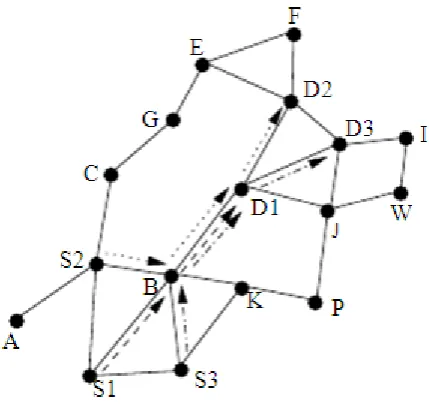
Fig. 1: Data packet flow using SP routing only.

(9)

number of flows and hops (which have also least number of flows and hops), then the preferred route is randomly selected.

When a source nodes has data to send, and a fresh (or active) route already exists or has been determined through a route discovery. Then a Flow ID is created and stored, and the data is forwarded to the next hop. Each forwarding node then creates their own flow IDs (as described previously) and continue for-warding the data packets. This process continues (including at the destination node) until the destination node is reached. Furthermore, each consequtive data packet are used to update the lifetime of each flow ID (if the flow ID already exists).

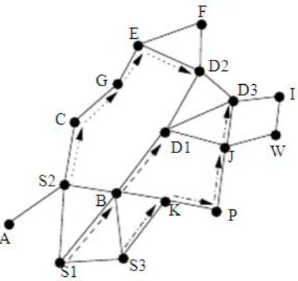
To illustrate how FSF algorithm works. Assume that F lowτ = 1 and S1, S2 and S3 (see Figure 1) want to send data to D1, D2 and D3. Using shortest path (SP) routing, all data packets travel through node B and D1 Thus creating possible performance bottlenecks at these nodes. In FSF (see Figure 2), the route discovery strategy uses a combination of data flows restriction and SP routing to distribute the packets through nodes C, B and K, instead of through node B only (as was the case in Figure 1). As a result, FARP ensures a better distribution of data traffic than using purely SP routing.

(10)

Fig. 2: Data packet flow using FSF.

Note in Xz, X represents the node ID and Z is the number of flows Fig. 3: Illustration of control overhead reduction in FARP.

Simulation Model

This section describes the scenarios and parameters used in simulation studies performed for FARP. It also describes the performance metrics used to compare FARP with a number of other existing routing strategies.

A. Simulation Environment and Scenarios

(11)

works. The simulations were performed for 10, 20 and 100 node networks, migrating in a 1000 m x 1000 m area IEEE 802 .11 DSSS (Direct Sequence Spread Spectrum) was used with maximum transmission power of 15dbm at a 2Mb/s data rate. In the MAC layer, IEEE 802.11 was used in DCF mode. The radio capture effects were also taken into account. Two - ray path loss characteristics was considered as the propagation model. The antenna hight was set to1.5m, the radio receiver threshold was set to -81 dbm and the receiver sensitivity was set to -91 dbm according to the Lucent wavelan card. Ran - dom way -point mobility model was used with the node mobility ranging from 0to20m/sandpausetimewassetto0seconds

Table I: FARP Simulation Parameters.

Flow Timeout 3s

Flow Expiration Time 2s Flow Threshold 8 RREQ Retry Times 6

For continuous mobility the simulations ran for 200s3 and each simulation was averaged over eight different simulation runs using different seed values.

Constant Bit Rate (CBR) traffic was used to establish communication between nodes. Each CBR packet was contained 512 Bytes and each packet were at 0.25s intervals The simulation was run for 5, 10, 20 and 40 different client/server pairs[4] and each session begin at different times and was set to last for the duration of the simulation.

The FARP routing protocols was implemented on the top of the AODV algorithm. Table I illustrates the simulation parameters used for FARP. Note that the Flow Timeout represents the timeout interval at which the flow table entries are updated. The Flow Expiration Time represents the lifetime of each flow. The Flow Threshold is used to assume a maximum number of flows at each node. This is used in the FSF algorithm. The RREQ Retry Times represents the number of times a source can initiate a route discovery before the destination is seen as unreachable.

B. Performance Metrics

The performance of each routing protocol is compared using the following performance metrics.

(12)

• End-to-End Delay

• Total Flows per Node (TFN)

PDR is the Ratio of the number of number of packets received by the destination to the number of packets sent by the source. Control overhead (O/H) presents the number of control packets transmitted through the network. The End-to-End Delay represents the average delay experienced by each packet when travelling from the source to the destination. The Total Flows per Node (AFN) represents the total number of data flows handled by each node in the network for the complete duration of the simulation. The above metrics where taken for different values of pause time.

RESULTS

This sections presents the results obtained for FARP and AODV, and provides a performance comparison between these protocols.

We kept the simulation time lower due to a very high execution time required for the 40 flow scenario.

Note that the terms Client/Server, src/dest and Flows are used interchange-ably.

(13)

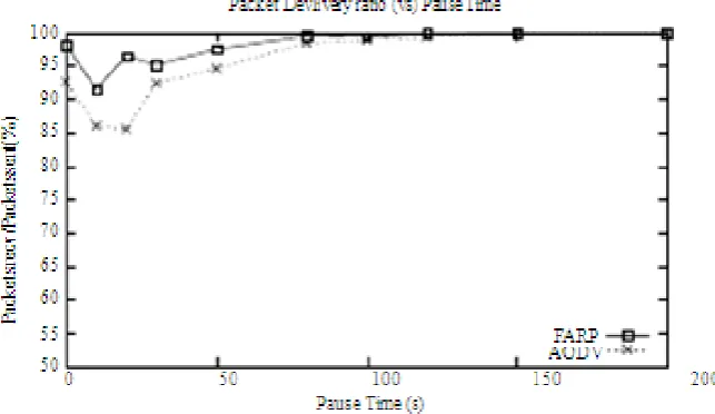
Fig. 5: PDR: 100 Nodes and 50 Flows.

(14)

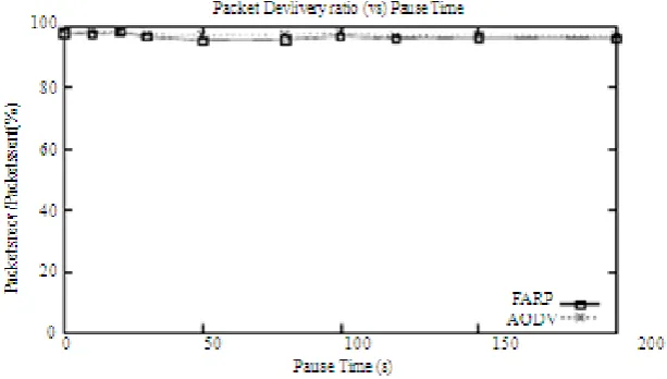
A. Packet Delivery Ratio

Figure 4 and 5 illustrate the PDR results obtained for the 20 and 100 node scenarios. These figures illustrate the packet de-livery performance of AODV and FARP in a small to medium sized mobile ad hoc network. In the 20 nodes scenarios both FARP and AODV achieve over 98% PDR. However, in the 100 node scenario it can be seen that FARP achieves a higher level of packet delivery than AODV when node mobility is high (i.e. for small pause times). This is because FARP reduces the probability of establishing routes over bottleneck (or saturated nodes). Therefore, the data packets would have a better chance of reaching the required destination in FARP than in AODV. Furthermore, FARP introduces a more selective approach to flooding than AODV. This means that not every node in the network would rebroadcast control packets. Hence, there is of-ten less channel contention between nodes and smaller chance of packets being lost due to interference and buffer overflows when compared to pure flooding.

B. Control Packets

Figure 6 and 7 illustrate the number of control packets introduced into the network for the 20 and 100 node scenarios respectively. In both scenarios it can be seen that FARP produces fewer control packets than AODV. This is more evident when mobility is high. This is because in high mobility both proto-cols initiate more route discoveries due to more frequent route failures. However, in FARP each route discovery may result in fewer number of control packet rebroadcasts than AODV, due to restriction of flooding over nodes which have fewer flows, which cuts down the number of rebroadcasting nodes when compared to AODV.

C. Delays

(15)

Fig. 8: Delays: 20 Nodes and 10 Flows.

Fig. 9: Delays: 100 Nodes and 50 Flows.

(16)

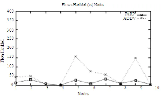
Fig. 11: TFN: 20 Nodes and 10 Flows.

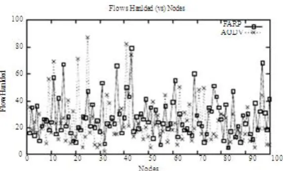
Fig. 12: TFN: 100 Nodes and 50 Flows.

D. Flow Distribution

(17)

node graph it can see that AODV still experiences the largest variation in flow distribution. For example, the smallest flow count experienced by a node in AODV is close to 0 and the largest is around 90, where as in FARP the smallest value is close to 8 and the largest is around 78 flows.

Alternative Strategies and Improvements Dynamic Flow Threshold Selection

In FSF algorithm, the flow threshold (The limit for the number of flows allowed at each node) was chosen as a simulation parameter. Therefore, each node in our simulations used a static value for the flow threshold. The disadvantage of a static flow threshold is that it may not always allow for the best flow distribution in the network. To make more accurate prediction of Flows Hanlded (vs) Nodes

Flow limits and better flows distribution each node must make these decisions dynamically based on the current conditions of the network. One way to calculate the flow threshold dynamically is through the use and exchange of neighbour flow information. In this strategy, each node exchange flow information with their neighbouring nodes (using hello packets) and calculates an average flow per neighbour and the maximum number of flows, which can be experienced by each node at each particular region. Using this information the first few RREQ propagations can be restricted to nodes, which are handling average or lower levels of flows.

B. Rate Adaptive Flow Timeout Selection

In our FARP simulations, the flows that are not refreshed every 2 seconds or less are deleted from the flow table. The disadvantage of this is different applications may be transmit-ting data at different rates. Therefore, by assigning a static Flow Timeout, the flow table may be storing each flow ID for a longer or shorter time than it is required. To overcome this, the Flow Timeout value can be set by observing the rate at which data packets arrive at each node and assigning a timeout value, which closely matches the expected arrival time.

CONCLUSIONS

(18)

nodes in the network. This is achieved by restricting the RREQ retransmission over the nodes, which have the least number of flows. We implemented FARP on the top of AODV and compared their performance by simulations. Our results show that FARP reduces the number of control packets transmitted through the network, while achieving better data flow distribution in the net-work. In the future, we plan to investigate the performance of FARP over large network with high levels of mobility.

REFERENCES

1. Mehran Abolhasan, Tadeusz Wysocki, and Eryk Dutkiewicz. LPAR: An Adaptive Routing Strategy for MANETs. In Journal of Telecommunication and Information Technology, 2003; 2: 28–37.

2. George Aggelou and Rahim Tafazolli. RDMAR: A bandwidth-efficient routing protocol for mobile ad hoc networks. In ACM International Work-shop on Wireless Mobile Multimedia (WoWMoM), 1999; 26–33.

3. B. Bellur, R.G. OGIER, and F.L Templin. Topology broadcast based on reverse-path forwarding routing protocol (TBRPF). In Internet Draft, draft-ietf-manet-tbrpf-06.txt, work in progress, 2003.

4. T-W. Chen and M. Gerla. Global State Routing: A New Routing Scheme for Ad-hoc Wireless Networks. Proc. IEEE ICC, 1998.

5. S. Das, C. Perkins, and E. Royer. Ad Hoc on Demand Distance Vector (AODV) Routing. In Internet Draft, draft-ietf-manet-aodv-11.txt, work in progress, 2002.

6. H. Hassanein and A. Zhou. Routing with load balancing in wireless ad hoc networks. In Proceedings of ACM MSWiM, Rome, Italy, july, 2001.

7. V. Wong J.-H. Song and V. Leung. Load-aware on-demand routing (laor) protocol for mobile ad hoc networks. In IEEE Vehicular Technology Conference (VTC-Spring), Jeju, Korea, 2003; 1753-1757.

8. P. Jacquet, P. Muhlethaler, T. Clausen, A. Laouiti, A. Qayyum, and L. Vi-ennot. Optimized link state routing protocol for ad hoc networks, ieee inmic Pakistan, 2001. 9. Yong-Bae Ko and Nitin H. Vaidya. Location-Aided Routing (LAR) in Mobile Ad Hoc

Networks. In Proceedings of the Fourth AnnualACM/IEEE International Conference on Mobile Computing and Networking (Mobicom’98), Dallas, TX, 1998.

(19)

11.S.J. Lee and M. Gerla. Dynamic load-aware routing in ad hoc networks. In Proceedings of ICC, Helsinki, Finland, June, 2001.

12.S.J. Lee and M. Gerla. Smr: Split multipath routing with maximally disjoint paths in ad hoc networks. In Proceedings of ICC, Helsinki, Finland, June, 2001.

13.Lucent. Orinoco pc card. In http://www.lucent.com/orinoco, 2003.

14.C.E. Perkins and T.J. Watson. Highly Dynamic Destination Sequenced Distance Vector Routing (DSDV) for Mobile Computers. In ACM SIG- COMM’94 Conference on Communications Architectures, London, UK, 1994.