Interactive Medical Image Registration With Multigrid Methods and Bounded Biharmonic Functions

University of Pennsylvania

ScholarlyCommons

Publicly Accessible Penn Dissertations

1-1-2014

Interactive Medical Image Registration With

Multigrid Methods and Bounded Biharmonic

Functions

Baohua Wu

University of Pennsylvania, [email protected]

Follow this and additional works at:

http://repository.upenn.edu/edissertations

Part of the

Computer Sciences Commons, and the

Radiology Commons

This paper is posted at ScholarlyCommons.http://repository.upenn.edu/edissertations/1502

For more information, please [email protected].

Recommended Citation

Wu, Baohua, "Interactive Medical Image Registration With Multigrid Methods and Bounded Biharmonic Functions" (2014).Publicly Accessible Penn Dissertations. 1502.

Interactive Medical Image Registration With Multigrid Methods and

Bounded Biharmonic Functions

Abstract

Interactive image registration is important in some medical applications since automatic image registration is

often slow and sometimes error-prone. We consider interactive registration methods that incorporate

user-specified local transforms around control handles. The deformation between handles is interpolated by some

smooth functions, minimizing some variational energies. Besides smoothness, we expect the impact of a

control handle to be local. Therefore we choose bounded biharmonic weight functions to blend local

transforms, a cutting-edge technique in computer graphics. However, medical images are usually huge, and

this technique takes a lot of time that makes itself impracticable for interactive image registration.

To expedite this process, we use a multigrid active set method to solve bounded biharmonic functions (BBF).

The multigrid approach is for two scenarios, refining the active set from coarse to fine resolutions, and solving

the linear systems constrained by working active sets. We've implemented both weighted Jacobi method and

successive over-relaxation (SOR) in the multigrid solver. Since the problem has box constraints, we cannot

directly use regular updates in Jacobi and SOR methods. Instead, we choose a descent step size and clamp the

update to satisfy the box constraints. We explore the ways to choose step sizes and discuss their relation to the

spectral radii of the iteration matrices. The relaxation factors, which are closely related to step sizes, are

estimated by analyzing the eigenvalues of the bilaplacian matrices. We give a proof about the termination of

our algorithm and provide some theoretical error bounds.

Another minor problem we address is to register big images on GPU with limited memory. We've

implemented an image registration algorithm with virtual image slices on GPU. An image slice is treated

similarly to a page in virtual memory. We execute a wavefront of subtasks together to reduce the number of

data transfers.

Our main contribution is a fast multigrid method for interactive medical image registration that uses bounded

biharmonic functions to blend local transforms. We report a novel multigrid approach to refine active set

quickly and use clamped updates based on weighted Jacobi and SOR. This multigrid method can be used to

efficiently solve other quadratic programs that have active sets distributed over continuous regions.

Degree Type

Dissertation

Degree Name

Doctor of Philosophy (PhD)

Graduate Group

Computer and Information Science

First Advisor

James C. Gee

Second Advisor

Norman I. Badler

Keywords

Active set, Bounded biharmonic functions, Graphics animation, Medical image registration, Multigrid

methods, Virtual GPU memory

Subject Categories

Computer Sciences | Radiology

INTERACTIVE MEDICAL IMAGE REGISTRATION WITH MULTIGRID METHODS AND

BOUNDED BIHARMONIC FUNCTIONS

Baohua Wu

A DISSERTATION

in

Computer and Information Science

Presented to the Faculties of the University of Pennsylvania

in

Partial Fulfillment of the Requirements for the

Degree of Doctor of Philosophy

2014

Supervisor of Dissertation

_________________________

James C. Gee

Associate Professor of Radiologic Science

Graduate Group Chairperson

_________________________

Val Tannen, Professor of Computer and Information Science

Dissertation Committee

Norman I. Badler, Professor of Computer and Information Science

Camillo J. Taylor, Professor of Computer and Information Science

Ladislav Kavan, Assistant Professor of Computer and Information Science

INTERACTIVE MEDICAL IMAGE REGISTRATION WITH MULTIGRID METHODS AND

BOUNDED BIHARMONIC FUNCTIONS

COPYRIGHT

2014

iii

iv

ACKNOWLEDGMENT

First I would like to express my sincere gratitude to my supervisor, Dr. James Gee for his

insightful guidance, continuous care, and precious support. It is a privilege for me to receive

numerous instructions from him and to contribute on the exciting areas identified by him.

I would like to extend my heartfelt gratitude to my co-advisor, Dr. Camillo Taylor, who

introduced me to this area and gave me a lot of advice. I am also grateful to Dr. Norman Badler

for being the chair of my dissertation committee, Dr. Ladislav Kavan and Dr. Dimitris Metaxas for

serving on my committee and offering insightful directions.

I would like to express my sincere thanks to Dr. Brian Avants, Dr. Alec Jacobson and Dr.

Gang Song who greatly inspired me in research. In addition, I would also like to thank Profs.

Honghui Lu, Insup Lee, Sampath Kannan, Linda Zhao, Lawrence Brown, Zhijie Li, Shoko Nioka,

Britton Chance, Jianbo Shi, Jean Gallier, Gary Zhang, Yuanjie Zheng, Paul Yushkevich and other

faculty who helped me in the past few years.

In addition, I would like to express my great thanks to my close friends, Y. Wen, J. Chen, H.

Xu, J. Yan, C. Kuo, Z. Yang, L. Ma, X. Zhang, W. Wu, T. Li, and many others for their continuous

care and help.

Also I would like to express my heartfelt gratitude to my wife, for her tremendous help,

precious love and continuous support, to my mother for her everlasting care and

encouragements, and to my father for intriguing my interest in mathematics during my childhood.

Finally I would like to dedicate this dissertation to Dr. Yan. I am deeply grateful for his

v

ABSTRACT

INTERACTIVE MEDICAL IMAGE REGISTRATION WITH MULTIGRID METHODS AND

BOUNDED BIHARMONIC FUNCTIONS

Baohua Wu

James Gee

Interactive image registration is required in some medical applications since automatic image

registration is often slow and sometimes error-prone. We consider interactive registration

methods that incorporate user-specified local transforms around control handles. The deformation

between handles is interpolated by some smooth functions, minimizing some variational energies.

Besides smoothness, we expect the impact of a control handle to be local. Therefore we choose

bounded biharmonic weight functions to blend local transforms, a cutting-edge technique in

computer graphics. However, medical images are usually huge, and this technique takes a lot of

time that makes itself impracticable for interactive image registration.

To expedite this process, we use a multigrid active set method to solve bounded biharmonic

functions (BBF). The multigrid approach is for two scenarios, refining the active set from coarse to

fine resolutions, and solving the linear systems constrained by working active sets. We've

implemented both weighted Jacobi scheme and successive over-relaxation (SOR) in the multigrid

active set method. Since the problem has box constraints, we cannot directly use regular updates

as in classic Jacobi and SOR methods. Instead, we choose a descent step size and clamp the

update to satisfy the box constraints. We explore the ways to choose step sizes and discuss their

relation to the spectral radii of the iteration matrices. The relaxation factors, which are closely

related to step sizes, are estimated by analyzing the eigenvalues of the bilaplacian matrices. We

give a proof about the termination of our algorithm and provide some theoretical error bounds.

Another minor problem we address is to register big images on GPU with limited memory.

vi

slice is treated similarly to a page in virtual memory. We execute a wavefront of subtasks together

to reduce the number of data transfers.

Our main contribution is a novel numerical method named multigrid active set to efficiently

solve bounded biharmonic functions, which are quadratic programs with inequality functions. The

bounded biharmonic functions are used to blend local transforms for interactive medical image

registration. We report an original multigrid approach to refine active set quickly and use clamped

updates based on weighted Jacobi and SOR. The multigrid active set method can be used to

efficiently solve other quadratic programs that have active sets distributed over continuous

vii

TABLE OF CONTENTS

ACKNOWLEDGMENT

... IV

ABSTRACT

... V

LIST OF TABLES ... X

LIST OF ILLUSTRATIONS ... XI

CHAPTER 1

INTRODUCTION ... 1

1.1 Image Registration ... 2

1.2 Interactive Image Registration ... 3

1.3 Linear Blend Skinning with Bounded Biharmonic Weights ... 4

1.4 Contributions ... 6

1.5 Dissertation Organization ... 8

CHAPTER 2

BACKGROUND ON DIFFERENTIAL GEOMETRY ... 9

2.1 Curves and Surfaces ... 9

2.2 Euler-Lagrange Equation ... 13

2.3 Variational Deformation Energies ... 15

2.4 Thin-plate Splines ... 16

2.5 Discrete Beltrami-Laplace Operator ... 18

2.5.1 Discrete Beltrami-Laplace Operator by Finite Elements ... 19

2.5.2 Discrete Beltrami-Laplace Operator by Finite Differences ... 24

2.6 Bounded Biharmonic Functions ... 26

CHAPTER 3

EXISTING METHODS SOLVING BOUNDED BIHARMONIC

FUNCTIONS 28

3.1.1 Lagrange Multiplier Method ... 28

viii

3.1.3 Karush–Kuhn–Tucker Conditions ... 30

3.1.4 Convex Optimization and Slater's Condition ... 31

3.2 Active Set Method for Convex Quadratic Programming... 33

3.2.1 Relation between Negative Lagrange Multipliers and Descent Directions ... 33

3.2.2 Active Set Method ... 35

3.2.3 Convex Quadratic Program of Bounded Biharmonic Functions ... 38

3.3 Linear Systems for the Bounded Biharmonic Functions ... 39

3.3.1 Methods Solving the Linear Systems ... 41

3.3.2 Cholesky Decomposition... 41

3.3.3 Minimum Degree Algorithms ... 42

3.4 Interior Point Method... 45

3.5 Summary ... 47

CHAPTER 4

MULTIGRID ACTIVE SET METHOD WITH GRADIENT DESCENT 49

4.2 The Aggressive Active Set Algorithm ... 51

4.2.1 Lagrange Multipliers of Bounded Biharmonic Functions ... 51

4.2.2 Eigenvalue Ranges of Principle Minors ... 53

4.2.3 Aggressive Active Set Method with Clamped Descent Steps ... 55

4.2.4 Termination of the Aggressive Active Set Algorithm ... 58

4.3 Summary ... 64

CHAPTER 5

MULTIGRID ACTIVE METHODS WITH JACOBI AND SOR SCHEMES

66

5.1.1 Weighted Jacobi Scheme ... 66

5.1.2 Multigrid Iterative Methods ... 70

5.2 Eigenvalues of Discrete Laplacian Matrices... 72

5.3 Weights of the Jacobi Scheme for Bounded Biharmonic Functions ... 73

5.4 Relation between Jacobi Scheme and Gradient Descent ... 75

5.5 Clamped Jacobi Scheme on Triangular Meshes ... 76

5.6 Clamped SOR Scheme on Triangular Meshes ... 81

5.7 Error Bounds and Computational Complexity ... 82

ix

CHAPTER 6

IMPLEMENTATION AND EXPERIMENTAL RESULTS ... 87

6.1 Implementation ... 87

6.1.1 Matlab Prototype on Cartesian and Triangular Meshes of 2D ... 87

6.1.2 C++ Prototype on Cartesian Meshes of 2D and 3D ... 87

6.1.3 Memory Usage ... 88

6.1.4 Adjacent Handles ... 89

6.2 Use Cases with Medical Images ... 90

6.2.1 Interactive Registration of an MR image and an histological image... 90

6.2.2 Interactive Registration of 3D MR Brain Images ... 92

6.2.3 Interactive Registration of Histology Images with Tears ... 94

6.3 Comparison to Existing Methods ... 95

6.4 Further Expeditions ... 99

6.4.1 Skip Updates on Mesh Vertices inside Regions of Active Sets ... 99

6.4.2 Adaptive Subdivision According to Curvatures and Approximation Errors ... 102

6.5 Summary ... 104

CHAPTER 7

GPU MEMORY MANAGEMENT FOR IMAGE REGISTRATION ... 105

7.1 GPU Memory Hierarchy ... 105

7.2 Virtual Image Slices on GPU ... 107

7.3 Demons Image Registration with Virtual Image Slices ... 108

7.4 Wavefront Execution for Multiple Iterations ... 112

7.5 Experimental Results ... 114

7.6 Discussion ... 116

CHAPTER 8

CONCLUSION ... 118

8.1 List of Contributions ... 119

8.2 Future work ... 120

A

APPENDIX... 122

A.1 Error Bounds of Multigrid Relaxation on Cartesian Meshes ... 122

x

LIST OF TABLES

xi

LIST OF ILLUSTRATIONS

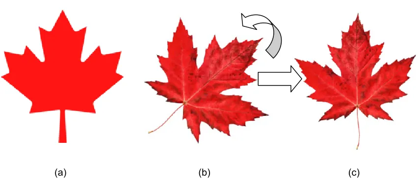
Figure 1.1: (a) a template of maple leaves. (b) a maple leaf before registration. (c) after a 45º

anticlockwise rotation, the maple leaf is registered to the template. ... 1

Figure 2.1: Left: vertex

wi

and its neighboring shaded region for Laplacian integral. Middle:

Laplacian integral over the shaded triangle is zero since the gradient is constant. Right: Laplacian

integral over the reduced shaded region. ... 19

Figure 2.2: Linear basis function B

shown as the slope with value 1 at w

, and 0 at w

and w

... 20

Figure 2.3: Left: a triangular mesh in a two dimensional domain. Right: A tent function

ϕi

defined

at a mesh vertex near the center of the domain. ... 23

Figure 2.4: Left: a thin-plate spline that has value 1 at one handle and value 0 at other handles.

Right: a bounded biharmonic function (BBF) with the same values at handles. BBF is favored

since it decreases over distance to the peak handle and has a local support. ... 27

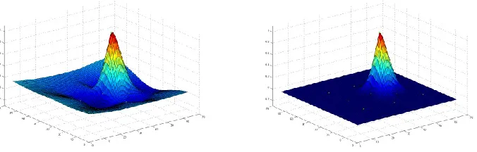
Figure 4.1: Active set regions at different resolutions are similar except minor differences at

region boundaries. The blue regions are active sets with values 0, and the dark red dots are

active set with values 1. Left: mesh spacing

h=1/32

; right:

h=1/64

. ... 50

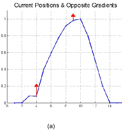
Figure 4.2: Solid curves are the current position, and dashed curves are the updated position. (a)

the current function values and opposite gradients showed in arrows. (b) regular update with

uniformly scaled gradients. (c) aggressive update with non-uniformly scaled gradients. ... 56

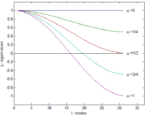
Figure 5.1: The eigenvalues of the weighted Jacobi iteration matrix.

: the weights.

-axis: the

indices of the modes.

-axis: the eigenvalues. ... 70

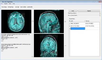
Figure 6.1: A snapshot of the interactive registration prototype with two 3D MR images of brains

being loaded. The purple markers are the locations of user-defined landmarks. ... 88

Figure 6.2: A histological image is warped to align with a MR image. In the bottom image, the +

signs are the locations of control handles. The deformation field is blended from local

xii

1

Chapter 1

Introduction

Image registration is a process to align multiple images. The images may be taken from different

subjects, at different times, from different perspectives, or with different imaging methods. With

image registration, we discover the spatial correspondences between pixels in one image and

pixels in another.

Figure 1.1 shows an example of image registration. The left image is a template of maple

leaves and the middle image is a skewed maple leaf that doesn't overlap well with the template.

With an anticlockwise rotation of 45º, we get a maple leaf standing up straight in the right image.

After rotation, the left and right images are well aligned, and the correspondences between the

pixels in the two images are established.

(a) (b) (c)

Figure 1.1: (a) a template of maple leaves. (b) a maple leaf before registration. (c) after a 45º

anticlockwise rotation, the maple leaf is registered to the template.

Image registration has been widely used in medical image analysis, such as voxel-based

morphometry, atlas-based segmentation, neuronal connectivity analysis, image guided therapy,

2

automatic registration methods are often time-consuming and sometimes error-prone. In some

situations, it is more desirable to use interactive image registration that is guided by interactive

directions from human being.

1.1

Image Registration

We will give a formal definition of image registration. Given a fixed image and a moving image

defined over a spatial domain , an image registration process tries to find an optimal

transform that satisfies some regularization conditions [1] and warps into

such that is similar to . The similarity is measured by some distance function

, and the regularization by another function . In other words, an image registration

solves the following optimization problem [1-3]:

(1.1)

where is a constant for the weight of regularization. In some references, the fixed image is

called the reference image, and the moving image is called the template image.

Generally speaking transforms can be categorized into affine transforms and non-affine

transforms. Specific affine transforms include translation, rotation, scaling and shearing. When

only translation and rotation are considered, it is called rigid transform. Non-affine transforms can

model complex deformations, including free-form deformations [1, 4], pixel-wise displacement

fields [5, 6], landmark-based splines, etc. In practice, an image registration process often finds an

affine transform first for global alignment, and after that, it looks for non-affine transforms to align

local details.

The similarity term can be defined in many ways, such as Sum of Squared Differences of

intensities (SSD), Correlation Coefficient (CC) [7], Normalized Cross Correlation (NCC), Gradient

Correlation (GC), Mutual Information (MI), Normalized Mutual Information (NMI), etc [2, 8]. SSD is

3

are used when the intensities of two images have some linear correlation. MI-based methods

works well for images with very different intensity distributions, for example, when they are

acquired from different modalities, such as CT and MRI [9].

The regularization term usually promotes the smoothness of the transform that may be

defined with some differential operators. Depending on the order of derivatives, we have

stretching energy (1st order), bending energy (2nd order), curvature variation energy (3rd order),

etc [10, 11]. Examples of bending energy are thin plate energy [1] and Laplacian energy [6].

1.2

Interactive Image Registration

Interactive image registration has been used in some clinical applications, such as minimally

invasive surgeries [8] and image guided radiotherapy (IGRT) [12, 13]. Before a surgery, a

preoperative image is acquired with by CT or MRI, and a surgical region of interest (ROI) is drawn

based on some expert knowledge. During the surgery, some intraoperative images are acquired,

for example, by ultrasound, and then registered to the preoperative image to track the location of

ROI dynamically.

Automatic image registration usually takes minutes to hours with the current multi-core CPUs

since medical images are often of large volumes. Even worse, the volumes have been increasing

due to the development of medical imaging devices with higher resolutions. Such processing time

is acceptable for some offline image analysis, but is far from being satisfactory for interactive

applications since a surgeon can't wait for ten minutes to find out the new position of an organ

after a body movement.

For performance, we choose landmark-based registration where a user can specify the

correspondences of landmarks between the fixed and moving images. We interpolate the

deformation between landmarks to produce a displacement field. Afterwards, this field is used as

the initial parameters for automatic registration that will move image pixels locally for small scale

4

Landmark-based registration can improve the quality of automatic registration as well. It

remains a challenge to find a global optimum solution for image registration, even with affine

transforms. When the affine registration gets stuck with a local optimum solution, it will be

extremely difficult for a follow-up non-affine registration to produce a good alignment.

In medical images, landmarks are usually feature points that are meaningful in biology or

geometry, for example, anterior commissure (AC) and posterior commissure (PC) in brain MR

images. When landmarks are specified in a pair of images under registration, their

correspondences define the displacements from the fixed landmarks to the moving landmarks.

We can infer the displacements over the whole image domain with a method called scattered

data interpolation [14-17].

The task of scattered data interpolation is to find a smooth function that has given function

values at a set of control handles , that is,

(1.2)

This function is often represented as a weighted sum of radial basis functions centered at control

handles [14, 18], in the following form

(1.3)

where φ is a radially symmetric function, and is the weight for the -th handle. A radial basis

function is often called a kernel. Some common kernels include Gaussian function, multiquadratic

functions, and thin plate splines.

With interactive image registration, some expected affine transforms, instread of function

values, are defined at the scattered handles. Our task is to interpolate the deformation at the

locations other than the handles. To accomplish this task, we use linear blend skinning (LBS), a

well-known method in computer graphics [19, 20].

5

In graphic animation, skinning is a process to attach a skin to a moving skeleton that has joints

and bones. The movement of a joint is usually defined by an affine transform. A skin vertex is

attached to one or multiple joints, and the movement of a skin vertex is derived by the movement

of joints to which it attaches.

As a popular skinning method, linear blend skinning (LBS) blends affine transforms defined

on joints with some weight functions. Assume that we are given affine transforms around

control handles , for . The impact of each control handle is specified by some weight

functions . Linear blend skinning of these affine transforms are defined by

(1.4)

For blending quality, Jacobson et al. suggest that the weight functions have some properties

including locality, smoothness, non-negativity, partition of unity, decreasing over distance, etc [21,

22]. Jacobson et al. proposed to use bounded biharmonic weights (BBW) based on finite

elements and bending energies [22, 23]. By enforcing some box bounds, for example , the

resulting biharmonic weights satisfies the desirable properties.

For smoothness, the weight functions minimizes the following energy [21] :

(1.5)

where ∆ is the Laplacian operator and is the domain.

It is natural that the impact from a handle to a location is measured by a value between 0 and

1. With value 1, we mean that the handle has full impact at that location. With value 0, we mean

that the handle has no impact over there. Usually we expect that a handle has full impact at itself

and no impact at other handles. Therefore, we require that the weight function for the -th

handle satisfies the following conditions:

(1.6)

6

where is the Kronecker delta function.

Furthermore, it is commonly required that the weights from all handles sum to one at each

location. In other words, we expect partition of unity, that is,

(1.8)

When all handles move with a same translation, this condition will ensure that other points to be

translated in the same fashion.

With finite elements, the smooth energy (1.5) can be discretized and represented in a

quadratic form with unknown variables being the weight values over the domain. The formulae

(1.5) - (1.8) defines a quadratic program that is expensive to solve.

To expedite the computation, Jacobson et al. reduced the problem size by solving each

weight function separately. To keep the partition of unity, it normalize the weights afterwards:

When is near handle , is almost one, and other are almost zero. Therefore,

is almost biharmonic near , and almost zero at remote places. The normalized

bounded biharmonic weights (BBW) will approximate well the exact solution. According to the

authors, the experimental results of this size-reduced problem are similar to the original problem

except at some remote regions far from handles.

1.4

Contributions

With finite elements, a bounded biharmonic function can be represented by a quadratic program

that are often solved by interior point methods and active set methods. Active set methods solve

the problem by a series of estimation of the active set that is the set of inequality constraints

7

system. In our case of medical image registration, there are more than millions of pixels.

Therefore, a direct use of the existing methods will take a lot of time and can't satisfy our

requirement of interactivity. To reduce the computation time, we solve this problem from a

multigrid approach.

Our main contribution is a fast numerical method of solving bounded biharmonic functions.

Specifically, our contribution includes the following aspects.

1. We report a novel multigrid approach to refine active sets in quadratic programming. For a

bounded biharmonic function, its active set is distributed over some continuous regions.

Therefore, the boundary of the active set can be quickly refined from coarser levels to finer levels.

2. We present technical details of multigrid iterative methods to solve bilaplacian linear

systems. We use clamped update of weighted Jacobi iteration and successive over-relation and

report the proper parameters according the ranges of eigenvalues.

3. We use adaptive subdivision to refine the triangular meshes according to the curvature. A

biharmonic function tends to be linear at locations far from control handles. For these

approximately linear regions, much fewer mesh vertices are needed, and other points can be

computed by linear interpolation.

We implemented the methods above within Matlab and solved bounded biharmonic functions

in less than a few seconds for a domain with millions of pixels. Besides our Matlab experiments,

we implemented a C++ prototype based on ITK, Qt, and OpenGL. And this prototype supports

Cartesian meshes on both 2D and 3D images.

Another problem we address is to handle limited memory of GPU when huge medical images

are registered automatically. We borrow the concept of virtual memory from operating system and

treat a block of image as a virtual page. We only load a few blocks onto GPU when they will be

needed soon. With this memory access manner, we are able to reduce the peak memory usage

8

1.5

Dissertation Organization

The remaining dissertation is organized into the following chapters. In Chapter 2, we will review

some variational deformation models, derive the discrete Laplacian operators, and define the

problem of bounded harmonic functions. In Chapter 3, we will introduce convex quadratic

programming, active set methods, interior point methods and linear solvers. In Chapter 4, we

report a multigrid approach to refine active sets, ways to clamp the gradient descent and an

aggressive strategy to update the working active set. In Chapter 5, we describe multigrid active

set methods with clamped updates from weighted Jacobi scheme and SOR. We also report some

parameters for convergence by analyzing eigenvalues of the discrete bilaplacian matrix. We

further give some theoretical error bounds with multigrid relaxation and discuss the computation

complexity. In Chapter 6, we present our implementations and experimental results. In Chapter 7,

we report a method that manages GPU memory to process big images. And we present an

enhancement to reduce the number of data transfers by compute the wavefront subtasks

9

Chapter 2

Background on Differential Geometry

2.1

Curves and Surfaces

Let us start with an example of a car moving on a horizontal plane. Imagine that on the plane

there are an x-axis from west to east and an y-axis from south to north. The car's position

can be represented by a function of time :

At a specific time t, the car's velocity can be computed by the derivative,

which is also the tangent vector of the curve. The curve length that the car

travels from time is the integral

(2.1)

When the car makes a turn, the "sharpness" of the turn describes how fast the velocity vector

changes direction. If we denote the angle between the velocity and -axis by , the sharpness

can be measured by the changing rate of over arc length . This rate gives a definition for the

curvature

(2.2)

Sometimes we use arc length to reparameterize the curve, which is called natural

parameterization. With parameter , the trajectory can be represented by function , and its

curvature is given by,

_(2.3)

Sometimes we don't have a parameter or . Instead, a planar curve is represented in an

10

(2.4)

For example, for a parabola , its curvature is at .

Let us consider a parametric surface embedded in a three

dimensional space. Given parameter changes around point , we

can define its tangent plane by first order approximation

(2.5)

where is its Jacobian matrix at defined by

(2.6)

When the parameters deviate from along a line specified by a direction vector

, we get a parametric curve by . From the chain rule of

derivatives, the directional derivative can be computed by

(2.7)

This also defines a tangent of the surface when the parameters changes on direction . The

length of this directional derivative is . For convenience, we name

(2.8)

the first fundamental form [24, 25]. For two direction vectors , the inner product of two

directional derivatives is . With this inner product, we can derive lengths, angles and areas

in the tangent space from vectors in the parameter space. For example, the area of a surface

11

(2.9)

If we approximate the surface near with second order derivatives, we have function

with each component being

(2.10)

where

. is the Hessian matrix of with .

If we consider in the Darboux frame defined by the tangent plane and normal vector at ,

the approximation becomes a paraboloid with its stationary point at . We project its

deviation from the tangent plane onto the unit normal n and get

(2.11)

where and are defined similarly. We call the matrix

(2.12)

by the second fundamental form [24, 25].

Let us consider again the directional curve . Its change projected on

the surface normal is approximately

12

Around , the arc length can be approximated by

according to Formula (2.8). Reparameterizing the directional curve with arc length , we have

According to Formula (2.3), its curvature at point can be computed by its 2nd

derivative w.r.t. :

This is called the normal curvature of the curve at the intersection of the surface and the plane

spanned by the directional derivative and the surface normal.

When the surface tangent rotates, the curvature achieves its maximum

and minimum . We call the principal curvatures. The Gaussian curvature is

defined by

(2.14)

If we denote the angle between the surface tangent and the by , the normal curvature

at direction is

according to Euler's theorem. If we consider two perpendicular tangents and , their angles

are different by and therefore . The sum of the normal curvatures is a

constant

We define a mean curvature over the all directions by

13

If we consider the symmetry of the curvatures over two opposite tangents, we have

We further rewrite it over all pairs of perpendicular tangents and compute the mean

curvature by

(2.15)

At a point on a surface, the mean curvature normal is defined by where is the normal

vector at the point.

The mean curvature normal can be evaluated by the Laplace-Beltrami operator that we

will discuss later in this chapter. Briefly speaking, the Laplace-Beltrami operator is an extension of

Laplace operator to the coordinate function of the surface.

2.2

Euler-Lagrange Equation

In Formula (2.1), we've defined the length of a parametric curve by differentiation. When the

curve is represented by an explicit function , we may treat it as a

parametric curve with being the parameter, and its arc length can be computed by

(2.16)

In some problems, boundary conditions are known in advance, and

our goal is to find a function that minimizes the length . This problem can be solved by its

Euler-Lagrange equation.

Generally speaking, we have a functional where is a function

defined on , is its derivative, and is a real-value function with partial derivatives.

For a function to be a stationary point of , must satisfy the Euler-Lagrange equation

14

When is a vector , we have a system of equations replicating the above with

replaced by . When is a vector , the Euler-Lagrange equation becomes

(2.18)

where . The Euler-Lagrange equation gives the necessary condition for a function to

be a local extremum [26].

Let us go back to the problem of finding a function with minimal length given boundary

conditions. Substituting (2.16) into (2.17), we get

Therefore, must be a constant. In other words, must be a line passing the end points defined

by the boundary conditions.

In a more complicated case, the second derivative of is also an argument of the function

_{. The Euler-Lagrange equation becomes [26]} (2.19)

When

, the Euler-Lagrange equation is given by

(2.20)

15

2.3

Variational Deformation Energies

Again with the example of driving a car, we say the road is rough if it has a lot of ups and downs.

In mathematics, we can measure "ups and downs" by the integral of squared variations

(2.21)

where f(x) is a height function of location x in a horizontal domain Ω and is its gradient. When

the gradient is zero everywhere, we have a flat road with a constant height. The smoothness

formula (2.21) is called the Dirichlet energy.

When the road crosses a river, we would like to build a bridge touching the two river banks at

locations a and b. Assume the bank heights at a and b are f1and f2respectively. In general, for a

function defined on domain , we may know in advance its values at boundary by

(2.22)

which is called Dirichlet boundary condition.

Sometimes we also know the gradient of in advance at boundary . More precisely, we

have

(2.23)

where n is the (outgoing) normal at the boundary . This is called Neumann boundary condition.

Applying Euler-Lagrange equation (2.18) to Dirichlet energy (2.21), the function minimizing

this energy must satisfy

(2.24)

which is called the Laplace's equation. The operator is called the Laplacian operator. A function

16

As we have discussed in Section 2.1, the curvatures of a surface can be derived from its

second order partial derivatives. If we define a curvature-related energy, we should include 's

second derivatives in the functional. A well-known example is the thin-plate energy [27, 28] that

may model the bending behavior of a thin steel plate under some force. For a 2D plate, we may

describe its deflection as a function . Its thin-plate energy is defined

as

(2.25)

Applying formula (2.20), we get its Euler-Lagrange equation

(2.26)

where is the bilaplacian operator or biharmonic operator. The equation is referred to as the

biharmonic equation, and a function satisfying the biharmonic equation is called a biharmonic

function.

Another energy based on second order partial derivatives is Laplacian energy defined by

(2.27)

It can be easily verified that its Euler-Lagrange equation is the same as that of thin-plate energy.

In general we can include higher order partial derivatives in the smooth energy [29].

2.4

Thin-plate Splines

The biharmonic equation has many solutions, and thus more conditions are required to decide a

specific solution. For example, we may require that the function values are given at scattered

points. The problem is to find a smooth function such that

17

It is not required that has continuous fourth-order partial derivatives at the scattered points

[30]. Instead the biharmonic equation is satisfied in a distributional sense, i.e.

where is a coefficient and is the Dirac delta function. If we ignore temporarily, the solution

to is the Green's function of the Laplace's operator. Denoting the

distance by for , we have where is a coefficient

depending on and is of the forms

(2.28)

Defining coefficients , we have the solution of the biharmonic equation in a

distributional sense

(2.29)

The function with this form is referred to as the thin-plate splines. And the functions are

called the radial basis functions of the thin-plate splines.

Since linear functions are the nullspace of plate energy, we would like to expand the

thin-plate splines to include them

(2.30)

where _{is the -th component of and are some}

unknown coefficients. To satisfy at scattered points, we have a linear system of the

coefficients where are the stacked vector of respectively, is

the stacked matrix of , and . Since we have more unknown

coefficients than the number of equations, we would like to add as some "orthogonality"

18

which has the solution

_y

The minimal thin-plate energy is .

Sometimes it is not required the function values follows strictly the expected values at

scattered points. The solution for this type of "soft" constraints is called smoothed thin-plate

splines [32]. We can define an soft constraint energy by

and define the overall energy by

where is weighting factor. The solution minimizing is similar to that of except we

substitute for .

2.5

Discrete Beltrami-Laplace Operator

In a discrete scenario, we define a mesh over the domain and approximate the differential

operator by function values at mesh vertices. Denote the function value at a mesh vertex by

and 's 1-ring neighborhood by . A simple definition of the discrete Beltrami-Laplace

operator at is to average the differences between and its 1-ring neighbors.

(2.31)

where is the number of vertices in the neighborhood [33]. In this definition, all vertices in the

1-ring neighborhood are treated equal. Although it is easy to compute, it often produces

19

2.5.1

Discrete Beltrami-Laplace Operator by Finite Elements

A more precise computation is the well-known cotangent Laplacian matrix that approximates the

discrete Beltrami-Laplace operator on triangular meshes by the finite element method. Let us

consider a surface defined by an explicit function,

. We triangulate its domain with a mesh made of vertices and triangles

. With the finite element method, the surface function is

approximated by a function that is piecewise linear over each mesh triangle.

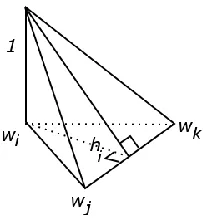
(a) (b) (c)

Figure 2.1: Left: vertex wi and its neighboring shaded region for Laplacian integral. Middle:

Laplacian integral over the shaded triangle is zero since the gradient is constant. Right: Laplacian

integral over the reduced shaded region.

As shown in Figure 2.1, a mesh vertex is adjacent to 6 vertices and 6 triangles. We would

like to estimate the mean Laplacian around by integrating its Laplacian over a neighborhood

around . There are a few ways for defining its neighborhood, for example, Voronoi cells and

barycentric cells. Here we choose barycentric cells where its neighborhood is connected by the

triangle barycenters and edge middle points, as shown in the shaded area in Figure 2.1a.

In Figure 2.1b, the shaded small triangle is formed by the two edge middle point

and the triangle barycenter . Since the gradient is constant over , we have

Ai

Dijk

20

Deducting all such small triangles from the neighborhood , we get a reduced neighborhood ,

as shown in Figure 2.1c. And we have

Since the Laplace's operator is the divergence of the gradient, we can compute the Laplacian

integral by the divergence theorem:

where is the outgoing normal on the boundary . Partitioning the boundary by all

adjacent triangles , we have

(2.32)

Next we will find out how to compute the gradient . For triangle with vertices ,

we define three linear basis functions corresponding to vertices . The linear

basis function has value 1 at and value 0 at other vertices , as shown in Figure

2.2. are defined in a similar way.

Figure 2.2: Linear basis function Bi shown as the slope with value 1 at wi, and 0 at wj and wk

Inside triangle , the piecewise linear function can be represented by the basis functions

21

where are the surface values at the vertices. Immediately

we have the gradient of

.

Therefore, we need to find out the gradients of the basis functions. Take as an example.

We denote the vector pointing from to by . The gradient of a basis function, for

example , can be computed by

(2.33)

where is the height of vertex in triangle , is the area of triangle , and means a

counter-clock-wise rotation of [34].

Since is linear and is equal to constant , we have

Therefore . Together with (2.33), the gradient of over triangle

is

Substituting the gradient into Formula (2.32), we get

Denote the angles at inside triangle by respectively. Double area of is

22

The first term inside the square bracket above is . Similarly the second term is

. Therefore, we have

Averaging the integral over the neighborhood area , the discrete Laplacian operator at

vertex can be approximated by

(2.34)

where and are the angles opposite to edge in the two adjacent triangles [34].

Applying the above equation over all vertices , we get a discrete approximation of Laplacian

operator on the triangle mesh

_(2.35)

where , is a diagonal matrix with , and is a symmetric matrix

with cotangent elements:

(2.36)

The diagonal matrix is also called the mass matrix.

Here we denote the cotangent matrix with the subscript to mean "stiffness". It is the

23

Figure 2.3: Left: a triangular mesh in a two dimensional domain. Right: A tent function ϕi defined

at a mesh vertex near the center of the domain.

Assume we have a function that has zero values at and outside the boundary of a

sub-region . Given a triangle mesh with vertices , function can be approximated

by a piecewise linear function . As shown in Figure 2.3, each

basis function is nonzero around vertex with a "tent" shape that has peak value one at

vertex and zero at the 1-ring neighbors and outside. Inside each triangle, linearly

interpolates its values at triangle vertices. The gradient of in each triangle incident to can be

evaluated with the same formula as (2.33). With a few derivation steps, we have

as defined in Formula (2.36). Please refer to [36] for the details of derivation.

Theorem 2.1: Given a set of tent functions , its stiffness matrix is symmetric

positive definite .

Proof: It is symmetric by formula (2.33). Given any function values defined on inside , we

can construct a piecewise linear function . We arrange values into a

24

Therefore is semi-positive definite. If , we must have over . Since

for any on the boundary , we have over the whole domain . That

means all . So is symmetric positive definite.□

Notice that this theorem is still true for a sub-region even with "holes" since any principal

minor of a positive definite matrix is still symmetric positive definite. Another way to understand it

is that the stiffness matrix is actually the Gram matrix of some basis functions.

2.5.2

Discrete Beltrami-Laplace Operator by Finite Differences

Since our images are often sampled over a regular grid, it is natural to use finite difference to

approximate the discrete Beltrami-Laplace operator. As a specific type of regular grids, Cartesian

grids have unit squares or cubes in the grid. Let us consider a 2D Cartesian grid of size

and a function that is zero on the boundary. A discrete Beltrami-Laplace operator at

vertices inside the boundarycan be defined as

where the subscripts are the vertex indices on the grid, and is the function value at vertex

. We arrange by dictionary order into a vector

and arrange in the same order into a vector . We have a linear system of

variables

25

where with for each edge and for each vertex . The

Laplacian matrix is a sparse matrix in this form:

with

It is interesting to observe that there is a connection between the Laplacian matrix from

finite difference and the cotangent Laplacian matrix _{. If we further partition the squares in}

the grid into triangles by parallel diagonals, we get a triangle mesh induced by the Cartesian grid.

Since the barycenter area around each vertex is constant one, is an identity matrix. In addition,

the angles inside each triangle are with cotangents respectively. We

have

(2.38) This equation holds for 3D cubic meshes if we partition each cube around its diagonal in a

rotational symmetric fashion [36].

Theorem 2.2: For a Cartesian grid in 2D or 3D, its Laplacian matrix defined by finite

difference are symmetric negative definite.

Proof: According to Theorem 2.1, is symmetric positive definite. Therefore is

symmetric negative definite. □

Sometimes we would like to exclude some control handles from consideration since

26

get a principal minor that is still symmetric positive definite. There are multiple ways to prove its

negative definiteness. We choose to explain it as the stiffness matrix (i.e. Gram matrix) of the

basis functions in the finite element method since this explanation also works for triangular

meshes.

2.6

Bounded Biharmonic Functions

In the previous chapter, we briefly introduced linear blend skinning with bounded biharmonic

weights. According to Formula (2.35), with a triangular mesh we can discretize the Laplacian

energy of a weight function as below.

As a reminder, is the partitioned area around vertex , is a diagonal matrix with diagonal

elements , and is the cotangent stiffness matrix. When there is no confusion, in the

future we will drop the subscript in .

The problem of solving the bounded biharmonic weight function of the -th handle becomes a

quadratic program that minimizes the following energy:

_(2.39)

subject to

and

27

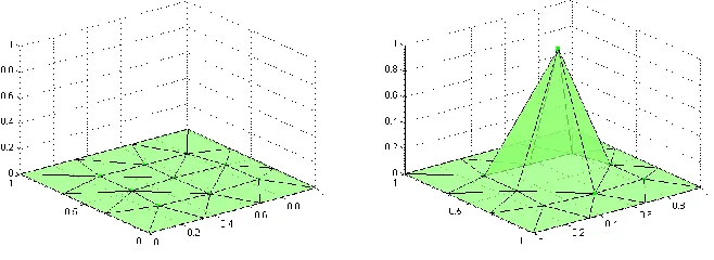
Figure 2.4: Left: a thin-plate spline that has value 1 at one handle and value 0 at other handles.

Right: a bounded biharmonic function (BBF) with the same values at handles. BBF is favored

since it decreases over distance to the peak handle and has a local support.

We may wonder why we don't use thin-plane splines that have a closed-form solution. One

reason is that thin-plate splines don't strictly decrease with the distance, as shown in Figure 2.4.

This increasing-with-distance behavior makes thin-plate splines not intuitive in describing the

impact of a control handle. Another reason is that thin-plate splines usually have an unbounded

support, which is not proper for our medical application where a handle has little impact over long

distance or at infinity.

A main difference of BBF from thin-plate splines is that there are inequality constraints

. These constraints also requires expensive computation since it is a quadratic

program.

It is easy to shown that the matrix _{is symmetric and positive definite. Remember}

that is a diagonal matrix with positive diagonals. For any vector , we have

If , we must have . Since is positive definite, is also nonsingular. We

must have =0. Since is symmetric and positive definite, the bounded biharmonic function

28

Chapter 3

Existing Methods Solving Bounded Biharmonic

Functions

In this chapter, we will review two popular methods, active set and interior point, for convex

quadratic programming. The active set method is chosen since the matrix of the quadratic form

has is sparse and symmetric positive definite. After the active set is estimated, the problem

becomes a linear system that can be quickly solved by Choleksy decomposition. Interior point

method is chosen since it has been used in commercial solvers, ex. MOSEK. We will explain that

the interior point method will solve a series of linear systems that share the same nonzero

structure in their system matrices. The same structure offers the space for expedition.

3.1

Introduction to Convex Optimization

3.1.1

Lagrange Multiplier Method

Lagrange Multiplier method gives the necessary conditions for some optimization problems. Let

us start with an optimization problem with equality constraints:

_(3.1)

with subject to

where are functions with continuous partial derivatives.

We construct a Lagrange function by introducing some auxiliary variables

The stationary points of the Lagrange function satisfy

29

The first condition above is the constraints in the original problem. The second condition above

says that the gradient of must be in the linear space spanned by the gradients of for

. It is easy to understand the first condition being necessary for to be optimal, but it is not

straightforward to understand the second condition.

Let us start our explanation about the second condition by assuming there is an optimum

solution at . Generally speaking, when has a very small change , a function has a

small change . The gradient gives the fastest changing direction. If is

orthogonal to gradient , the function stay unchanged. Since satisfies all equality

constraints, a "legal" change such that is still legal must satisfy for all

. Otherwise at least one constraint must be violated. Let a "violating" subspace

and a "legal" subspace where represents the orthogonal

complement of a subspace. In other words, a legal must be in the "legal" subspace .

Next we decompose by direct sum with . If let

changes a very little on the direction of , all constraints remain valid, but will be changed

by . This means is not a minimizer, and we have reached a

contradiction. So we must have . Therefore, . That

is, it is necessary to have the second condition holds for some .

3.1.2

Lagrange Dual of Optimization Problems

The Lagrange function can be extended to optimization problems with inequality constraints. A

general optimization problem may be written in the form:

(3.2)

subject to

30

The above constraints are called explicit constraints. The implicit constraint is that must be in

the intersection of the domains of the objective function and constraint functions. The intersection

gives the domain of this problem

A solution is said to be feasible if it is in and it satisfies all explicit constraints. We denote the

optimal solution by if it exists.

We define the Lagrange function of the general optimization problem by

and its Lagrange dual function [37] by

When (i.e. for all ), the dual function gives a lower bound on the optimal

value . This is because we have

Therefore, from the Lagrange dual problem

we can find a good lower bound for [37].

For distinction, we call the original problem the primal problem. We denote the optimal value

of the dual problem by , the optimal value of the primal problem by . We always have weak

duality . When , we say that it has strong duality.

3.1.3

Karush

–

Kuhn

–

Tucker Conditions

31

When strong duality ( holds, both " " signs become " " signs. When the first inequality

holds for equality, we have minimizing . Taking derivatives of w.r.t. , we

have

Since are feasible, we have . Therefore

and . When the second inequality holds for equality, we must have for

all . Thus we have

This is called complementary slackness.

In summary, for an optimization problem in (3.2) with strong duality and continuous

differentiable objective and constraint functions, if and are optimal solutions for the

primal and dual problem respectively, must satisfy the following the conditions:

(1) Primal constraints: and ,

(2) Dual constraints: ,

(3) Vanishing gradient: ,

(4) Complementary slackness: .

These conditions are called Karush-Kuhn-Tucker conditions or KKT conditions [38]. We call a

solution a KKT point if there are some such that satisfy the KKT conditions.

32

Convex optimization is a specific class of optimization that requires the objective function and

the feasible domain to be convex. A convex optimization problem can be written in the following

standard form:

_(3.3)

with subject to

where the objective function and the inequality constraint functions are convex, and the

equality constraints are affine. Inequality constraints are called boxed constraints or box bounds if

they are in the form where are some constants.

We have strong duality for a convex optimization problem if it has a strictly feasible solution.

By "strictly feasible" we mean a feasible solution satisfying

This is called the Slater's constraint qualification for strong duality of convex problems.

When a subset of are affine functions, the Slater's constraint qualification may

have a weak form by allowing that some affine constraints holds with equality signs, i.e.,

[37]. Most convex optimization problems have strong duality since it is easy for Slater's

condition to be satisfied for these problems.

Recall that the KKT conditions are necessary conditions for the optimizers of some

optimization problems. For convex problems, the KKT conditions are also sufficient conditions if

the objective and constraint functions have continuous derivatives. To show this, we assume that

satisfies the KKT conditions. Since the objective and constraint functions are

differentiable and convex, the Lagrange function must be differentiable and convex w.r.t.

33

satisfies the KKT conditions, we have , and must minimize

. Therefore, we have

The last equation holds because by complementary slackness and by

primal feasibility. Since with always gives a lower bound for the optimal , when

the equality sign holds as shown above, and are optimal solutions for the dual and

primal problems respectively.

In summary, when a convex optimization problem satisfies Slater's condition and its objective

and constraint functions have continuous partial derivatives, the KKT conditions are sufficient and

necessary conditions for its optimum solution.

3.2

Active Set Method for Convex Quadratic Programming

3.2.1

Relation between Negative Lagrange Multipliers and Descent Directions

Let us consider a convex quadratic programm minimizing

(3.4)

where is positive semi-definite matrix with subject to some affine constraints

We further assume that the constraint gradients are linear independent.

Since all inequality constraints are affine, it satisfies the weak form of Slater's condition if

there is a feasible solution in . Therefore, the KKT conditions are sufficient and necessary for

optimality.

For this convex quadratic program, any local optimal solution must be also globally

34

segment [ lies inside the feasible region that is a convex set, is a convex

function w.r.t. and achieves its minimum at . For any ,

. That is, is not a local optimum and we have a contradiction.

Let us consider a more restricted problem by requiring the equalities to hold for the inequality

constraints in the above problem.

(3.5)

subject to

We assume is a KKT point of problem (3.5) together with some Lagrange multipliers

. If it happens that for all , we can easily verify that also

satisfy the KKT conditions of the less constrained problem (3.4).

If there exists for some 1 , we will explain that is not a locally optimal solution

of problem (3.4) and there is feasible descent direction from . Since we assume that constraint

gradients are linear independent, cannot be expressed by any linear

combination of other gradients . Thus we can find a nonzero

direction where is the orthogonal projection of

gradient onto the linear space spanned by . Letting

, we have

Let us introduce a change with a positive that is small enough. For the -th constraint,

will change by and the -th constraint won't be violated. For any

-th constraint o-ther -than , and the constraint remains valid. We call such a

feasible direction since is feasible for some positive . By the KKT conditions

of problem (3.5), we have _{. Therefore, the objective function will change}