University of Pennsylvania
ScholarlyCommons
Publicly Accessible Penn Dissertations
1-1-2015
Essays on Bayesian Macroeconometrics
Molin Zhong
University of Pennsylvania, [email protected]
Follow this and additional works at:
http://repository.upenn.edu/edissertations
Part of the
Economics Commons
This paper is posted at ScholarlyCommons.http://repository.upenn.edu/edissertations/1173 For more information, please [email protected].
Recommended Citation
Zhong, Molin, "Essays on Bayesian Macroeconometrics" (2015).Publicly Accessible Penn Dissertations. 1173.
Essays on Bayesian Macroeconometrics
Abstract
This dissertation consists of three chapters that study the determinants of macroeconomic fluctuations, with a particular emphasis on the roles of agents' expectations and assessments of risks. In the first chapter, I study a business cycle model where the probability of transitioning to a downturn state characterized by low growth evolves over time. I call a change in the future probability of transitions to the downturn state a downturn risk shock. An increase in the risk of the downturn state leads to declines in consumption, investment, output, and hours. I take the model to the data using Bayesian methods. The fluctuations caused by expectations changes from the downturn risk shock account for substantial output variations at business cycle frequencies and hours fluctuations at medium run frequencies. The extracted time-varying probability process from the model matches well with the University of Michigan Index of Consumer Sentiments (ICS). Impulse response functions from downturn risk shocks produce the same comovement as those from ICS innovations in a structural vector autoregression. The second chapter, co-authored with Minchul Shin, proposes the
multivariate stochastic volatility in vector autoregression model as a framework for studying the real effects of uncertainty shocks. We advance a new approach to structurally identify uncertainty shocks that does not rely on identification of the level structural shocks. We estimate the model using a Bayesian Markov chain Monte Carlo algorithm, and we show how to construct impulse response functions and variance decompositions that can be used to analyze identified uncertainty shocks. The third chapter, also co-authored with Minchul Shin, suggests using ``realized volatility'' as a volatility proxy to aid in model-based multivariate bond yield density forecasting. To do so, we develop a general estimation approach to incorporate volatility proxy information into dynamic factor models with stochastic volatility. We study the density prediction performance on U.S. bond yields of including realized volatility into a dynamic Nelson-Siegel (DNS) model with stochastic volatility. The results clearly indicate that using realized volatility improves density forecasts relative to popular specifications in the DNS literature that neglect realized volatility.
Degree Type
Dissertation
Degree Name
Doctor of Philosophy (PhD)
Graduate Group
Economics
First Advisor
Jesus Fernandez-Villaverde
Keywords
Subject Categories
ESSAYS IN BAYESIAN MACROECONOMETRICS
Molin Zhong
A DISSERTATION
in
Economics
Presented to the Faculties of the University of Pennsylvania
in
Partial Fulfillment of the Requirements for the
Degree of Doctor of Philosophy
2015
Supervisor of Dissertation
Jes´us Fern´andez-Villaverde Professor of Economics
Graduate Group Chairperson
George Mailath, Professor of Economics
Dissertation Committee
ESSAYS IN BAYESIAN MACROECONOMETRICS
c
COPYRIGHT 2015
ACKNOWLEDGEMENTS
I cannot express how grateful I am to have Professor Jes´us Fern´andez-Villaverde as my
advisor. Professor Fern´andez-Villaverde guided me through the arduous process of becoming
a researcher in economics. He always was there to offer me his advice and wisdom. Most
importantly, through my time with him, I have learned the importance of positive thinking
and belief in myself. These are lessons that I will take with me beyond the profession and
I thank him dearly for instilling them in me.
I would like to thank Professors Francis Diebold and Frank Schorfheide. Professor Diebold
spent the time to introduce me into the profession when I was still an undergraduate. He
provided me the opportunity to attend Penn and I could always count on him to give helpful
guidance and productive comments. Professor Schorfheide pushed me further to improve
my work. He provided invaluable feedback on my dissertation to help me take it to the
level it is at today. I am lucky to have them on my committee.
My gratitude goes out to the members of the Penn Econometrics lunch group and the
economists at the Federal Reserve Banks of Philadelphia and St. Louis. I thank both the
Federal Reserve Bank of Philadelphia and the Federal Reserve Bank of St. Louis for their
hospitality.
I am especially indebted to Pablo Guerron-Quintana, who provided me useful direction
and support throughout my final years in the program. I would also like to thank George
Alessandria, Xu Cheng, Frank DiTraglia, Thorsten Drautzburg, and Edison Yu for many
helpful comments and feedback.
Thank you to the wonderful friends I have made along the process: Alessandro Arloto,
Lorenzo Braccini, Yumi Koh, Laura Liu, Yang Liu, Daniel Neuhann, Qiusha Peng, Devin
roommate for three years and Devin for being a great officemate for four years. I am
exceptionally thankful to my coauthor Minchul. Quoting the words of my advisor about
his coauthor: you are ”the best coauthor I could have hoped for.”
Finally, I would like to thank my parents and sister for their support during my time at
Penn. I could not have made it this far without them.
Molin Zhong
Philadelphia, PA
ABSTRACT
ESSAYS IN BAYESIAN MACROECONOMETRICS
Molin Zhong
Jes´us Fern´andez-Villaverde
This dissertation consists of three chapters that study the determinants of macroeconomic
fluctuations, with a particular emphasis on the roles of agents’ expectations and assessments
of risks. In the first chapter, I study a business cycle model where the probability of
transitioning to a downturn state characterized by low growth evolves over time. I call
a change in the future probability of transitions to the downturn state a downturn risk
shock. An increase in the risk of the downturn state leads to declines in consumption,
investment, output, and hours. I take the model to the data using Bayesian methods.
The fluctuations caused by expectations changes from the downturn risk shock account
for substantial output variations at business cycle frequencies and hours fluctuations at
medium run frequencies. The extracted time-varying probability process from the model
matches well with the University of Michigan Index of Consumer Sentiments (ICS). Impulse
response functions from downturn risk shocks produce the same comovement as those from
ICS innovations in a structural vector autoregression. The second chapter, co-authored
with Minchul Shin, proposes the multivariate stochastic volatility in vector autoregression
model as a framework for studying the real effects of uncertainty shocks. We advance a new
approach to structurally identify uncertainty shocks that does not rely on identification of
the level structural shocks. We estimate the model using a Bayesian Markov chain Monte
Carlo algorithm, and we show how to construct impulse response functions and variance
decompositions that can be used to analyze identified uncertainty shocks. The third chapter,
also co-authored with Minchul Shin, suggests using “realized volatility” as a volatility proxy
to aid in model-based multivariate bond yield density forecasting. To do so, we develop
factor models with stochastic volatility. We study the density prediction performance on
U.S. bond yields of including realized volatility into a dynamic Nelson-Siegel (DNS) model
with stochastic volatility. The results clearly indicate that using realized volatility improves
density forecasts relative to popular specifications in the DNS literature that neglect realized
TABLE OF CONTENTS
ACKNOWLEDGEMENTS . . . vi
ABSTRACT . . . vii
LIST OF TABLES . . . xi
LIST OF ILLUSTRATIONS . . . xiii
CHAPTER 1 : Variable Downturn Risk . . . 1
1.1 Introduction . . . 1
1.2 Stylized facts . . . 9
1.3 Simple model . . . 16
1.4 Structural estimation . . . 32
1.5 Conclusion . . . 61
1.6 Appendix . . . 63
CHAPTER 2 : A New Approach to Identifying the Real Effects of Uncertainty Shocks 78 2.1 Introduction . . . 78
2.2 Model . . . 82
2.3 Bayesian Analysis of CAIW-in-VAR Models . . . 86
2.4 Empirical Application: Real effects of financial volatility . . . 92
2.5 Conclusion and Future direction . . . 99
2.6 Appendix . . . 101
CHAPTER 3 : Does Realized Volatility Help Bond Yield Density Prediction? . . . 110
3.1 Introduction . . . 110
3.2 Model . . . 113
3.4 Estimation/Evaluation Methodology . . . 122
3.5 Results . . . 124
3.6 Conclusion . . . 135
3.7 Appendix . . . 137
LIST OF TABLES
TABLE 1 : Quarterly per capita output, consumption, and investment growth
1953Q2−2011Q4 . . . 9
TABLE 2 : Average quarterly declines in macroeconomic aggregates across NBER-designated recession periods . . . 12
TABLE 3 : Quantile regression forecast results . . . 14
TABLE 4 : Calibration simple economy . . . 17
TABLE 5 : Downturn risk shocks parameter calibration . . . 20
TABLE 6 : News shocks parameter calibration (m= 4) . . . 26
TABLE 7 : Fixed parameters . . . 41
TABLE 8 : Probability shock estimated parameters posterior intervals . . . 43
TABLE 9 : Variance decomposition at business cycle frequencies . . . 47
TABLE 10 : Variance decomposition at medium cycle frequencies . . . 47
TABLE 11 : Model-implied skewness . . . 48
TABLE 12 : Variance decomposition of pure downturn risk shock . . . 54
TABLE 13 : Log marginal likelihood comparison . . . 59
TABLE 14 : Variance decomposition of productivity news shock . . . 59
TABLE 15 : Variance decomposition of labor supply shock . . . 60
TABLE 16 : Comovements from SVAR versus expectations shocks . . . 61
TABLE 17 : Quantile regression forecast results . . . 64
TABLE 18 : Simulated data estimates . . . 70
TABLE 19 : Priors for downturn risk shocks model . . . 71
TABLE 20 : Posterior for downturn risk shocks model . . . 72
TABLE 21 : Posterior Estimates for CAIW(1)-in-VAR(4) . . . 109
TABLE 23 : Variance explained by the first five principal components (%) . . . 122
TABLE 24 : Posterior Estimates of Parameters onht Equation . . . 126
TABLE 25 : RMSE comparison . . . 128
TABLE 26 : Log predictive score comparison . . . 129
TABLE 27 : Log predictive score comparison: p-values . . . 130
TABLE 28 : RMSE comparison: Empirical factors . . . 134
TABLE 29 : Log predictive score: Empirical factors . . . 135
LIST OF ILLUSTRATIONS
FIGURE 1 : Histogram of forecast errors AR(1) model output growth . . . 11
FIGURE 2 : Time series of forecast errors AR(1) model output growth . . . . 13
FIGURE 3 : Impulse response to 1 standard deviation decrease in Index of Con-sumer Sentiments . . . 15
FIGURE 4 : Impulse response of productivity growth . . . 23
FIGURE 5 : Impulse response of depreciation rate . . . 24
FIGURE 6 : Impulse responses of consumption and investment to pure down-turn risk shock . . . 27
FIGURE 7 : Impulse responses of consumption and investment to unrealized productivity growth news shocks . . . 29
FIGURE 8 : Impulse responses of consumption and investment to pure down-turn risk shock shutting down productivity growth and depreciation 30 FIGURE 9 : Impulse responses of consumption and investment to realization of downturn state . . . 31
FIGURE 10 : Smoothed probability process . . . 44
FIGURE 11 : Smoothed process ˜ptand Index of Consumer Sentiments . . . 45
FIGURE 12 : Smoothed consumption and output growth implied by only down-turn risk . . . 46
FIGURE 13 : Impulse response to downturn risk shock . . . 50
FIGURE 14 : Smoothed hours implied by only pure downturn risk . . . 51
FIGURE 15 : Impulse response to pure downturn risk shock . . . 52
FIGURE 16 : Impulse response to pure downturn risk shock: sensitivity to price and wage rigidity . . . 53
FIGURE 19 : Impulse response to realization of the downturn state . . . 56
FIGURE 20 : Output, consumption, and hours during the Great Recession from
data and implied by the model . . . 58
FIGURE 21 : IP growth and Chicago Fed National Financial Conditions Index
1973M1−2012M12 . . . 94 FIGURE 22 : Impulse responses of IP level to real activity and financial
uncer-tainty shocks . . . 96
FIGURE 23 : Impulse responses of NFCI to real activity and financial uncertainty
shocks . . . 97
FIGURE 24 : Percentage of total forecast error variance of IP growth explained
by real activity and financial uncertainty . . . 98
FIGURE 25 : Percentage of total forecast error variance of NFCI explained by
real activity and financial uncertainty . . . 98
FIGURE 26 : Estimated Stochastic Volatility, IP growth . . . 108
FIGURE 27 : Estimated Stochastic Volatility, Financial conditions index . . . . 108
FIGURE 28 : U.S. Treasury Yields . . . 121
FIGURE 29 : Stochastic volatility for bond yield factors . . . 125
CHAPTER 1 : Variable Downturn Risk
1.1. Introduction
In this paper, I study a business cycle model with variable downturn risk. This study
is motivated by the asymmetric nature of macroeconomic fluctuations. On U.S. data,
output, consumption, and investment growth decline rapidly during recessions but increase
gradually during expansions. Moreover, the chance of a recession changes over time. The
economy goes through decade-long stretches with weak growth and frequent, deep recessions
and decade-long stretches with strong growth and infrequent, mild recessions. Do agents
react to this variable risk of downturns? How important are agents’ assessments of downturn
risk to macroeconomic fluctuations?
I address these questions as follows. I first provide stylized facts suggestive of the presence
of downturn risk. Current dynamic equilibrium models have a difficult time accounting for
this new form of risk. I therefore add a tightly-parametrized time-varying probability of
transitions to a downturn state over which agents have rational expectations to an otherwise
standard business cycle model.
A variety of stylized facts point to the presence and importance of downturn risk.
Distribu-tions of output, consumption, and investment growth show a long downside tail, indicating
a downturn state with rapid declines in the variables. These rapid declines do not seem to be
dispersed uniformly across time but instead appear to have a component operative at longer
horizons associated with the medium-frequency cycle (32−200 quarters). For instance, the 1970s and early 1980s, a time period of high risk of energy shortages, had four deep
reces-sions with sharp decreases in the macroeconomic aggregates. On the other hand, during
the late 1980s into the mid 2000s, a time period that included the information technology
I also present evidence that agents react to this downturn risk. I show that the University
of Michigan Index of Consumer Sentiments (ICS), a survey-based index of consumer
expec-tations, forecasts the lower tail of one-quarter ahead real per capita consumption growth
innovations but not the median or upper tail. This asymmetry suggests that information
relevant for downturns in the economy, more so than for upturns, shape agents’
expecta-tions. Moreover, fluctuating agents’ expectations and beliefs themselves seem to matter. In
a vector autoregression (VAR) with the ICS and a variety of key business cycle variables,
identified innovations to the ICS lead to significant movements in macroeconomic variables.
Along with documenting the importance of agents’ expectations for business cycle
move-ments, the VAR also gives suggestive evidence as to the comovements expectations shocks
should produce in a structural model.
The model I present allows for two states of the world: a downturn state and a normal
state. I introduce a tightly-parametrized first-order Markov time-varying probability of
transitioning to the downturn state that agents understand. This time-varying transition
probability captures the changing downturn risks that agents face. Moreover, a highly
persistent probability process implies that the shock has implications for both business cycle
and medium-frequency cycle fluctuations. The modeling framework is flexible enough to
allow for downturn, upturn, or symmetric risks to operate, but the econometric estimation
clearly points to variable downturn risks as driving business cycles. The downturn state in
the model has low productivity growth and high depreciation whereas the normal state has
high productivity growth and low depreciation. A possible interpretation of low productivity
growth during downturns is that capital misallocation increases. High depreciation during
downturns could result from increased economic depreciation or obsolescence, as opposed
to physical depreciation, of the capital stock.
A shock to the probability of the downturn state occurring, which I call a downturn risk
chang-ments in observed economic fundamentals (for example: productivity, preferences, or
pol-icy). In line with the literature, my VAR results suggest that in response to an identified
negative innovation to the ICS, both consumption and investment decline (see, for example,
Beaudry and Portier (2006)). While expectations shocks in general have a notoriously
diffi-cult time producing comovement between consumption and investment in standard business
cycle models, as shown by Beaudry and Portier (2004), thepure downturn risk shock, which
captures a change in risk of the downturn state with no subsequent movements in
pro-ductivity or depreciation (a pure change in expectations), can generate such comovement
in an otherwise standard real business cycle model. Expected future productivity growth
declines reduce the incentive to consume immediately through the wealth effect but have
difficulties inducing a decline in investment. Expected future depreciation increases reduce
the incentive to invest, which help produce comovement between output, consumption, and
investment. Using the same model with the same parameterization, I show a variety of
news shocks cannot generate this comovement, illustrating the importance of having both
productivity growth and depreciation in the downturn risk shock.
Since my model falls into the class of Markov-switching dynamic equilibrium models, I
can solve it using the perturbation methodology as in Foerster, Rubio-Ramirez, Waggoner,
and Zha (2013). The time-varying probability process governing the downturn risk is a
discretization of an underlying continuous autoregressive process parametrized by a
persis-tence, standard deviation, and long-run mean parameter. In this way, I can account for
rich dynamics in downturn risk while keeping the model tightly parametrized.
I take a quantitative version of the model with competing structural shocks to U.S.
macroe-conomic data from 1960Q2−2011Q4 using Bayesian methods.
In the estimated model, the downturn risk shock is an important driver of fluctuations
at both the business and medium-frequency cycles. At business cycle frequencies (8−32 quarters), the downturn risk shock plays a dominant role in consumption fluctuations,
output (around 30 percent of fluctuations) and hours (around 25 percent of fluctuations)
movements. The downturn risk in the economy triggers a wealth effect that becomes a
main driving force of consumption. Moving to medium frequencies (32−200 quarters), as defined by Comin and Gertler (2006), the downturn risk shock becomes the dominant driver
of the macroeconomic aggregates, accounting for around 60 percent of output movements. A
downturn probability shock can be seen as a type of intertemporally correlated news shock.
Its propagation has two sources of persistence: persistence in the news and persistence in
the realizations. Therefore, the effects of a change in downturn risk can persist for a long
time, which make the shock a natural candidate for driving longer-horizon fluctuations.
Periods of frequent and deep recessions have high downturn risk with many transitions to
the downturn state. Because agents also understand the high downturn risk present in the
economy, the lower expectations produce a further drag on macroeconomic performance.
On the other hand, when the economy has low downturn risk, there are few transitions to
the downturn state, generating infrequent recessions. Agents also understand this low risk,
which further boosts economic activity.
The pure downturn risk shock is empirically important for business cycles and drives hours
fluctuations at lower frequencies. Moreover, an increase in the probability of the downturn
state associated with the pure downturn risk shock leads to transitory declines in output,
consumption, investment, and hours, a hallmark of business cycle fluctuations. The pure
downturn risk shock drives around 40 percent of the movements in hours at medium
fre-quencies, which drastically decreases the importance of the labor supply shock in matching
hours. The model therefore gives a new interpretation to labor supply fluctuations: they
come about due to changes in the assessments of agents of the downturn risk in the
econ-omy. Evidence outside of the structural model seems to suggest such a theory of hours
fluctuations. The ICS and hours comove well across the data sample. Moreover, variance
decomposition results from a structural VAR suggest that up to 70% of hours fluctuations
Finally, the estimated model aligns well with exogenous supporting evidence. The smoothed
downturn risk probability process comoves well with the Index of Consumer Sentiments. In
addition, the impulse response to the downturn risk shock generates the same comovement
in macroeconomic variables as the response to an innovation in the ICS from a
structurally-identified VAR, which is further reassuring for the interpretation. A competing productivity
growth news shock in the model, for instance, misses the investment and federal funds rate
movements. Moreover, a variety of estimated models with alternative popular specifications
for expectations shocks also do not match these comovements.
Given the importance of the downturn risk shock in historical business cycle fluctuations,
I then evaluate how well it can account for the recent Great Recession. This recession is
interesting because it represents a large break in the economy. The previous 20 years were
characterized by the Great Moderation, a time of lower variation in macroeconomic series
and two mild recessions. Many economists think of the Great Recession as marking the end
of the Great Moderation. Therefore, changing expectations and sentiments of agents could
play a large role in this uncertain time period. The downturn risk shock is an important
driver of movements in output, consumption, and hours across the recession. Shutting down
all of the other shocks and only having downturn risks operative leads to movements in the
three series consistent with the data. The pure downturn risk shock accounts for between
25−40% of the decline of the three series across the recession.
In summary, changes in agents’ assessments of the downturn risk in the economy drive
macroeconomic fluctuations in my model. I find that these downturn risks have an
impor-tant component operative at medium-frequency horizons while having significant
implica-tions at business cycle frequencies. Moreover, changes in expectaimplica-tions alone caused by the
evolving risks are empirically relevant for business and medium-frequency cycle
macroe-conomic fluctuations. These expectations changes are important because they produce
comovement between consumption, investment, output, and hours, a defining feature of
Related literature My work connects to the literature in five main areas.
First, there exists a large literature discussing the importance of signals about the future
for business cycle fluctuations. This literature can be divided into three general categories:
news, noise, and sentiments.
The news shocks of Beaudry and Portier (2004) capture the idea that agents respond to
future fundamentals in making their decisions. Davis (2007), Schmitt-Grohe and Uribe
(2012), Fujiwara, Hirose, and Shintani (2011), and Khan and Tsoukalas (2012) estimate
models evaluating the importance of news shocks in driving business cycles. The downturn
risk shock can be considered a type of news shock. It differs from the standard news shock
in four key aspects. First, the process underlying the downturn risk shock in principle
al-lows for downside, upside, or symmetric risks, whereas the news shock only considers the
symmetric case. Second, the papers above model news as certain events in the future. The
downturn risk shock, on the other hand, only changes the probabilities with which future
states of the world will occur. This allows the downturn risk shock to also account for
situ-ations where the agents’ expectsitu-ations change but the realized future observed fundamentals
do not. Third, the downturn risk shock combines two different types of news: productivity
growth and depreciation. I show this combination is key to generate comovement between
consumption and investment without resorting to large adjustment costs. Fourth, the
down-turn risk shock is a parsimonious way of modeling intertemporal correlation of news shocks,
as will be discussed in more detail.
Noise shocks of Barsky and Sims (2012) and Blanchard, L’Huillier, and Lorenzoni (2013)
characterize a situation where agents receive noisy signals about the future. A noise shock
changes agents’ expectations while not impacting the observed fundamentals of the economy
as the noise only affects the signals that agents receive. A pure downturn risk shock has
similarities to a noise shock in that the observed fundamentals of the economy do not change
found for a noise shock.
Angeletos and La’O (2013) develop a theory of sentiment-driven fluctuations where
dis-persed information opens the door to changes in agents’ beliefs as a driver of macroeconomic
aggregates. Angeletos, Collard, and Dellas (2014) embed this beliefs shock into real business
cycle and New Keynesian models and find that it is an important driver of fluctuations.
The downturn risk shock, in contrast to the sentiments shock, changes agents’ expectations
through the time-varying risks of a bad state of the world occurring. It does not require
dispersed information.
Second, my work connects to the disasters literature introduced into macroeconomic models
by Gourio (2012). In a theoretical model, he shows that time-varying probability of disasters
can explain a variety of asset price phenomena while simultaneously driving business cycle
movements. As opposed to the disaster states that Gourio (2012) considers, my model
focuses on time-varying risks of less extreme downturn states that occur during recessions.
The increased frequency of these downturn states observed in the data relative to the
frequency of disaster states facilitates econometric estimation.
Third, the downturn risk shock links to the idea of long run risks of Bansal and Yaron
(2004) and medium-frequency cycles as in Comin and Gertler (2006). In the context of
empirical dynamic equilibrium models, these ideas are usually modeled as trend productivity
growth shocks, as in Croce (2014), Barsky and Sims (2012), and Blanchard, L’Huillier, and
Lorenzoni (2013). Relative to these models, my model ties the medium-frequency cycle
to business cycle asymmetries. Also, the empirically relevant inclusion of a depreciation
component in the downturn risk shock allows for comovement between consumption and
investment from pure changes in expectations.
Fourth, on the methodological side, this paper relates to the literature on estimating
Markov-switching dynamic equilibrium models (Schorfheide (2005), Liu, Waggoner, and
That literature builds on the work of Hamilton (1989), which first advances the
Markov-switching model. Diebold, Lee, and Weinbach (1994) propose the Markov-Markov-switching model
with time-varying transition probabilities, which has gained much importance in
reduced-form work. Most papers in the area specify an observable variable driving the transition
probabilities (Filardo (1994)). By embedding the Markov-switching time-varying transition
probability process into a dynamic equilibrium model, it is possible to use the decisions of
the agents to infer the transition probabilities at a given point in time. Bianchi and Melosi
(2013) discuss how the Markov-switching framework can quite naturally model movements
in agents’ expectations but does not conduct any empirical evaluation. My paper shows the
empirical relevance of using Markov-switching methods to model agents’ expectations.
Finally, this paper relates to the literature on generating asymmetry in business cycle
mod-els. These papers fall into two broad classes: ones that generate the asymmetry using
exogenous shocks and ones that do so endogenously in the model. As my paper does
not focus on generating asymmetry in macroeconomic models, but rather on producing
expectations-driven business cycles via the interaction of time-varying downturn risks and
frictions in the model, it falls into the former class. Andreasen, Fernandez-Villaverde, and
Rubio-Ramirez (2013), Ruge-Murcia (2012a), and Ruge-Murcia (2012b) use innovations
drawn from a skewed distribution to capture the skewness in macroeconomic and financial
data. Relative to that literature, my framework can also account for the predictability of
downside shocks. It can capture the notion of time-varying risks of downside shocks and
agents reacting to these changing risks. Considering effects of asymmetric adjustment costs
(Kim and Ruge-Murcia (2009) and Aruoba, Bocola, and Schorfheide (2013a)), the zero lower
bound on macroeconomic fluctuations (Fernandez-Villaverde, Gordon, Guerron-Quintana,
and Rubio-Ramirez (2012) and Aruoba, Cuba-Borda, and Schorfheide (2013)), and the
impact of occasionally binding financial constraints (Guerrieri and Iacoviello (2013)), are
the mechanism by embedding it within a real business cycle model. Section 4 discusses the
solution method and conducts Bayesian estimation on a quantitative dynamic equilibrium
model. Finally, section 5 concludes.
1.2. Stylized facts
In this section, I review four stylized facts about business cycle fluctuations that are relevant
to the topic at hand. These stylized facts provide evidence that (1) a downturn state
into which the economy occasionally transitions exists, (2) the risks of transitions to the
downturn state change over time, (3) these downturn risks impact agents’ sentiments and
expectations, and (4) changes in agents’ sentiments and expectations in and of themselves
are an important driver of macroeconomic fluctuations.
1. Output, consumption, and investment growth are negative skewed.
One defining feature of the U.S. business cycle is the asymmetry across expansions and
recessions. Expansions tend to produce gradual increases in growth rates of
macroeco-nomic aggregates whereas recessions lead to sharp decreases. Many researchers have
noted this asymmetry in reduced-from work, including Neftci (1984), Hamilton (1989),
Morley and Piger (2012), and Aruoba, Bocola, and Schorfheide (2013a). From an
un-conditional perspective, the asymmetric business cycle leads to the aggregate series of
output, consumption, and investment growth exhibiting clear negative skewness1.
Series Skewness Kurtosis J-B test p-val
Output growth −0.64 4.70 <0.001 Consumption growth −0.95 6.45 <0.001 Investment growth −0.41 4.43 <0.001
Table 1 Quarterly per capita output, consumption, and investment growth 1953Q2−2011Q4
1
Table 1 displays the skewness and kurtosis of these three macroeconomic aggregates
along with Jarque-Bera tests of normality. They all feature strong negative skewness
and fail normality tests.
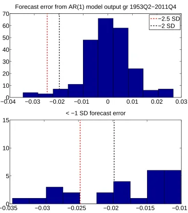
Figure 1 shows the forecast errors from fitting a simple AR(1) model to output growth
from 1953Q2−2011Q4. The forecast errors display a long left tail, mirroring the skewness found in the output growth data itself. Zooming in on this left tail, there
are 7 instances where the forecast errors fall less than 2.5 standard deviations below
the mean. This empirical fact suggests the presence of a downturn state into which
the economy occasionally transitions. For example, a normal distribution would rarely
generate so many observations so far below the mean2.
2. Frequencies and depths of recessions change over time.
The first stylized fact gives an unconditional statement about the asymmetry of
the U.S. business cycle. Looking beyond an unconditional perspective reveals the
long-horizon, changing frequency of rapid declines in the macroeconomic variables, as
pointed out by Comin and Gertler (2006) and dubbed the medium-frequency cycle.
They suggest that the economy enters decade-long stretches with poor macroeconomic
performance and frequent, deep recessions followed by decade-long stretches of robust
macroeconomic performance with infrequent, mild recessions. Across the 1950s into
the early 1960s, the U.S. went through three recessions with large declines in
out-put and investment growth. The mid-1960s, on the other hand, had strong economic
growth and was recession-free. From 1969−1982, the U.S. again reverted to a time period of poor economic performance. In a 13-year stretch, the U.S. went through four
recessions that produced large decreases in output and investment growth as well as
−0.040 −0.03 −0.02 −0.01 0 0.01 0.02 0.03 10
20 30 40 50 60 70
Forecast error from AR(1) model output gr 1953Q2−2011Q4
−2.5 SD −2 SD
−0.0350 −0.03 −0.025 −0.02 −0.015 −0.01 5
10 15
< −1 SD forecast error
of the deepest recessions in the sample, producing declines in the aggregates much
larger than the ”average” recession during any other period.
Series 1953−1961 (3 recessions) 1961−1969 (0 recessions) 1969−1982 (4 recessions)
Out gr −0.82% −− −0.87%
Cons gr 0.35% −− 0.05%
Inv gr −3.99% −− −3.53%
Series 1983−2006 (2 recessions) Great Recession
Out gr −0.45% −1.41%
Cons gr 0.26% −0.41%
Inv gr −2.70% −5.57%
Table 2 Average quarterly declines in macroeconomic aggregates across NBER-designated recession periods
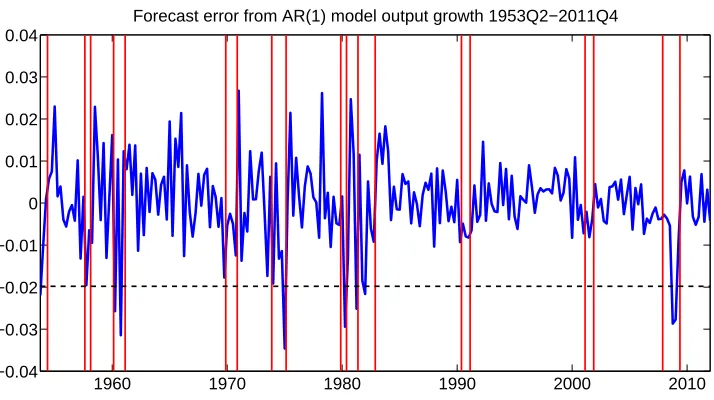
Moreover, deep recessions are associated with large downside shocks hitting the
econ-omy. Figure 2 shows that of the 7 recessions in the 1950s to early 1960s and late
1960s to early 1980s time frames, all but one are associated with innovations in
out-put growth lower than 2 standard deviations below the mean (<−2.0×10⁻²). The two mild recessions across the 1990s and 2000s, in contrast, do not have any such deep
1960 1970 1980 1990 2000 2010 −0.04
−0.03 −0.02 −0.01 0 0.01 0.02 0.03 0.04
Forecast error from AR(1) model output growth 1953Q2−2011Q4
Figure 2 Time series of forecast errors from AR(1) model fit with OLS to output growth. The red vertical lines denote NBER-dated recessions. The black horizontal dashed line gives the 2 standard deviations below the mean line.
3. Consumer sentiments movements are more associated with downturns in future
con-sumption growth innovations than upturns.
The University of Michigan Index of Consumer Sentiments is a popular proxy for
expectations and beliefs of consumers3. Barsky and Sims (2012) have shown a
re-lationship between the ICS and news about the future, suggesting that overall, the
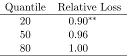
ICS has predictive content about future fundamentals. In this section, I document
an asymmetry of this predictive relationship by illustrating that the ICS forecasts
the 20th percentile of consumption growth innovations significantly better than the
historical quantile, but it does not forecast the 80th percentile significantly better.
This asymmetric relationship between the ICS and future downside innovations
sug-gests that information about downside risk in the economy is more relevant in forming
agents’ expectations relative to information about upside risk.
First, I fit an AR(1) with ordinary least squares to per capita consumption growth
3Papers such as Barsky and Sims (2012) and Angeletos, Collard, and Dellas (2014) have used elements
Quantile Relative Loss 20 0.90∗∗ 50 0.96 80 1.00
Table 3 Quantile regression forecast results for time t+ 1 consumption growth innovation given timet log Index of Consumer Sentiments. Using one-sided tests of higher predictive power of the sentiments model, ∗∗ indicates significance at the 5% level, and ∗ indicates significance at the 10% level.
data and extract the fitted innovations4. Then, I perform a quantile regression of
timetconsumption growth innovations (ˆct) on timet−1 log of consumer sentiments. Equation 1.1 gives the quantile regression specification for theτth quantile. My sample
runs from 1960Q2−2011Q4. ICS data availability restricts the beginning date of the sample. I begin one-quarter ahead forecasting at 1985Q3 and do an expanding window
recursive estimation until the end of the sample.
Qˆc
t(τ|logsentt−1) =α(τ) +β(τ) logsentt−1 (1.1)
1/NP
n
h ρτ
ˆ
ct+1−α˜(τ)−β˜(τ) logsentt
i
1/NP
n
ρτ ˆct+1−q˜(τ)
(1.2)
I choose the quantile loss function to evaluate the out-of-sample forecasts. Following
Giglio, Kelly, and Pruitt (2013), I present the loss using sentiments as a predictor
variable relative to the loss from the historical quantile. Equation 1.2 gives this
formula, where N is the number of forecasts and ρτ is theτth quantile loss function.
I assess significance using the Diebold and Mariano (2002) test of superior predictive
accuracy of the model with sentiments as a predictor variable given the two sequences
of forecast losses.
forecasting gain relative to using the historical quantile for the 20th percentile of
con-sumption growth innovations. This gain decreases moving to the median and entirely
disappears at the 80th percentile5. These results suggest that much of the
fluctua-tions in consumer sentiments comes from expectafluctua-tions about downside movements in
consumption as opposed to upside movements6. The current theoretical literature on
news shocks cannot address this asymmetry, but the downturn risk shock can.
4. Innovations in consumer sentiments have an impact on the economy.
0 20 40
−10 −5 0 5
ICS
0 20 40
−1.5 −1 −0.5 0
Cons
0 20 40
−4 −2 0 2
Inv
0 20 40
−1.5 −1 −0.5 0 0.5 Hours
0 20 40
−1 −0.5 0 0.5
Wage
0 20 40
−0.05 0 0.05 0.1
Infl
0 20 40
−0.15 −0.1 −0.05 0
FFR
Figure 3 Impulse response to 1 standard deviation decrease in Index of Consumers Senti-ments from a Bayesian VAR(4) on quarterly log University of Michigan Index of Consumers Sentiments (ICS), log per capita consumption, log per capita investment, log per capita hours, log per capita real wages, inflation, and federal funds rate. Responses are multiplied by 100. ICS is ordered first and a Cholesky identification strategy is used. Comovements of the impulse responses are robust to ICS ordered last. The blue lines are the pointwise median impulse responses whereas the red lines define the 68% credible set.
Figure 3 shows the responses to a 1 standard deviation negative Cholesky identified
5Results are robust to considering the 10th and 90th percentile. I have also tried using alternative
definitions of real consumption, deflating the series by the Consumer Price Index less food and energy as well as the Personal Consumption Expenditures price deflator. Full results are in the appendix.
6
shock to innovations in consumer sentiments from a VAR(4) composed of quarterly
log University of Michigan Index of Consumers Sentiments, log consumption, log
investment, log hours, log real wages, inflation, and federal funds rate. Consumption,
investment, hours, and real wages are in per capita values. Consumer sentiments are
ordered first. This VAR is similar in spirit to one found in Barsky and Sims (2012).
Details of the implementation of the VAR can be found in the appendix.
In response to the decline in sentiments, consumption, investment, and real wages
decrease permanently. On impact, consumption and investment both decline.
Invest-ment and labor supply both have hump-shaped components. Notice the long-lived
response of hours. Almost 25 quarters after an expectations shock, hours still have
not fully returned back to steady state. Inflation increases whereas the federal funds
rate declines. These responses are all significant, providing suggestive evidence that
changes in expectations of agents have important effects on the economy. Moreover,
the responses of the variables to the movements in expectations give guidance as to
how the model economy should react to expectations shocks.
1.3. Simple model
Given the stylized facts in the previous section, I now turn to illustrating how the downturn
risk shock can capture what is found in the data. I start with a real business cycle model
with capital and labor to clearly illustrate the properties of the downturn risk shock.
max
ct,it,kt+1,lt
E
∞ X
t=0
βt log (ct−hct−1)−ψ
l1+t γ
1 +γ !
s.t. ct+it=Atkαtl1t−α
kt+1 =it+ (1−δt)kt
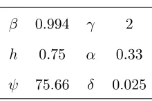
β 0.994 γ 2
h 0.75 α 0.33
ψ 75.66 δ 0.025
Table 4 Calibration simple economy
The social planner maximizes over consumption ct, investment it, capital kt+1, and
la-bor lt, subject to the resource constraint and capital accumulation equation. Agents have
seperable utility over consumption and labor. They value consumption relative to an
in-ternal habit level governed by h. The economy has a Cobb-Douglas production function
hit by productivity shocks At with growth rate gA,t. Depreciation of the capital stock δt
is stochastic depending upon the state of the world. Stochastic depreciation could come
from economic depreciation as in Greenwood, Hercowitz, and Krusell (1997) or economic
obsolescence as in Gertler and Kiyotaki (2010), Liu, Waggoner, and Zha (2011), and Gourio
(2012). Table 4 gives the calibrated parameters for the simple economy, which are relatively
uncontroversial7. I consider log-linear approximations to this model economy.
1.3.1. Markov-switching dynamics and the downturn risk shock
There are two observed states of the world, which I characterize as adownturn state(st= 1)
and a normal state (st = 2). The downturn state features low productivity growth and
high capital depreciation. This state occurs rarely in practice, but agents are aware of its
existence and the time-varying risks of transitioning to this state. The normal state has
7
high productivity growth and low capital depreciation.
gA,t= (1−ρA)ΛA+ρAgA,t−1+cA(st) +A,t, A,t∼N(0, σA2) (1.4)
logδt= logδ+d(st)
cA(st) =
cA(1)<0, d(1)>0 w.p.1−p(st−1)
cA(2)>0, d(2)<0 w.p. p(st−1)
EcA(s),Ed(s) = 0
Equation 1.4 lays out the productivity growth and depreciation processes. At timet, agents
know all variables datedtor earlier. ThegA,tprocess follows an AR(1), as is standard in the
literature. The variablecA(st) gives the low growth and high growth values of productivity
growth. Likewise, d(st) determines the level of capital depreciation across the states. The
unconditional means of these parameters are both 0, meaning that they represent deviations
around the long-run values. Agents at timetknow the probabilities of entering the normal
and downturn states in time t+ 1, given by p(st) and 1−p(st), respectively. Changes in
p(st), therefore, change the downturn risk that agents face. I introduce st to index the
probabilities with which the economy enters into the normal versus downturn states in the
following period. Crucially, notice that a change in this risk does not necessarily have to
coincide with a change in observed productivity growth or capital depreciation. It impacts
agents’ assessments of future prospects, however, and will therefore alter current behavior.
prob(st|st−1) =Q(st−1) (1.5)
Equation 1.5 specifies the dynamics for st. Specifically, the st states transition according
to a first-order Markov process. I allow for many probability states st. This leads to an
states means determiningN−1 +N(N−1) parameters8. To solve this issue, I specify the probability process as coming from an N-state Tauchen approximation of the AR(1)-type
process specified in equation 1.6.
pt=
ep˜t
1 +ep˜t (1.6)
˜
pt= (1−ρp)µp+ρpp˜t−1+p,t, p,t∼N(0, σ2p)
First, I discretize the process ˜pt into N states. Then, I apply the logistic transformation
to each discretized value to constrain each of them onto the unit interval. The Tauchen
approximation allows me to jointly determine the probability states and transition matrix
as a function of only three parameters: µp, ρp, σp, or the long-run mean, persistence, and
standard deviation of the underlying continuous process9.
Interpretation of downturn transition
The downturn state transition causes a decline in productivity growth and an increase in
de-preciation. Productivity growth could decline if misallocation increases during downturns.
The depreciation increase could capture heightened economic depreciation or obsolescence.
Historically, the two have often coincided. Economic obsolescence has been used by Gertler
and Kiyotaki (2010) as a driver of financial intermediation disruptions. If the reduced ability
of financial intermediation also impacts the economy’s ability to allocate capital efficiently,
productivity growth could also decline. Economic obsolescence has often been associated
with disruptions in financial intermediation. For instance, many consider the recent poor
financial conditions driving the downturn in the Great Recession as caused by a large
eco-nomic depreciation of the housing stock, which tightened bank balance sheets and disrupted
lending10. Oil supply shocks could also cause productivity growth and economic
obsoles-8
TheN−1 comes from the probability values of theNstates, whileN(N−1) from the transition matrix
Q. 9
Further details of the solution algorithm are in the Structural estimation section of the paper. 10
cence to move together. Changes in oil prices have been known to lead to large reallocations
across sectors11, which could lead to productivity declines if misallocation increases. If the
energy shocks lead to abandonment of energy-intensive capital, then economic depreciation
would also increase. As this paper focuses on agents’ reactions to changing risks of these
downturns, I abstract from a further explicit microfoundation of the relationship.
Analysis and simulation of the process
µp 2
ρp 0.88
σp 0.61
cA(1) (cA(2)) −0.009 (0.002)
d(1) (d(2)) 1.63 (−0.36)
ρA 0.2
σA 0.005
Table 5 Downturn risk shocks parameter calibration
Table 5 gives the illustrative calibration for the downturn risk shocks process. A key
pa-rameter of interest is µp, the long-run mean parameter. The sign ofµp determines whether
the process captures downturn risk or upturn risk. The logistic transformation ensures that
a value ˜pt = 0 gives exactly one half chance of transitioning to either state at timet+ 1.
Values of ˜pt>0 mean a higher probability of transitioning to the normal state while ˜pt<0
imply the opposite. A long-run mean of µp > 0 implies that the ˜pt process should spend
more time above 0, leading to a higher probability on average of transitioning to the normal
state. Unconditional expectations of cA(st) and d(st) both equalling 0 then imply that
|cA(1)| > |cA(2)|,|d(1)| > |d(2)|. This parametrization captures the intuition of a larger
magnitude, but relatively infrequent, downturn state and a smaller magnitude, but more
the illustrative calibration, I set the valueµp = 2, which leads to cA(st) and d(st) having a
rather large degree of asymmetry in deviations from steady state12.
The asymmetries in the process generate unconditional negative skewness for the
produc-tivity growth and positive skewness for the depreciation rate processes. For the calibration
above, the skewness of productivity growth is−0.25 while that of depreciation is 1.63. This asymmetry translates to asymmetry in the endogenous variables as well, to be discussed
in a following subsection. Therefore, the model can capture the asymmetry of the
busi-ness cycle. Deep recessions are associated with more frequent transitions to the downturn
state - or downside shocks - causing rapid decreases in the endogenous variables. Because
the probability of the downturn state occurring, given by p(st), is known by agents, the
downturn risk shock can capture the stylized fact that changes in agents’ expectations are
associated with downside innovations in the economy.
The parametersρp andρAgovern the persistence of the probability and productivity growth
processes, respectively. A higher value ofρp makes the probability process more persistent,
meaning that an increased probability of transitioning to the downturn state at timetleads
to higher probabilities of a downturn state for an extended period. IncreasedρAleads to a
longer propagation of realized productivity growth changes.
The interaction of the two parameters, however, can lead to many interesting shapes for
expected productivity growth as a result of a change in downturn risk. Equation 1.7, the
impulse response to a probability shock at time t, illustrates why this happens (Call ˆgA,t+k
the deviation of gA,t+k from its long-run mean.). An innovation to the probability process
does not change productivity growth at periodt. Increasing the probability of transitioning
to the downturn state, for example, means that at timet+1, there exists a higher probability
of a downturn state transition, loweringEtgA,t+1. One can think of this as timet+ 1 news.
12
Moving forward, there now exists two effects onEtgA,t+k. First, ifρp >0, there still exists
a higher probability of a transition to the downturn state, as the probability process has
persistence. Think of this as time t+k news. Second, with ρA >0, the previous period’s
conditional expectation of the process propagates forward because the gA,t process itself is
persistent as well. The first effect feeds into the second one, implying that a probability
shock can persist for quite some time. In fact, if ρA and ρp are persistent enough, the
impulse response of gA,t can even feature a hump-shape, increasing in the initial periods
before mean-reverting, a feature that innovations in a standard real business cycle model
cannot achieve.
ˆ
gA,t= 0 (1.7)
EtgˆA,t+1 = (1−p (1)
t )cA(1) +p
(1)
t cA(2)
| {z }
t+1 news
EtgˆA,t+2 =ρA((1−p(1)t )cA(1) +p(1)t cA(2)) + (1−p(2)t )cA(1) +p(2)t cA(2)
| {z }
t+2 news
...
Etgˆt+k= k
X
j=1
ρkA−j
(1−p(tj))cA(1) +p(tj)cA(2)
p(tn)=Etp(st+n−1)
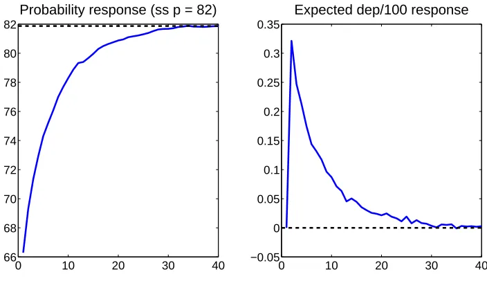
Figure 4 shows impulse responses of productivity growth to a decrease in p(st), which
makes the downturn state more likely. As both ρp and ρA are positive, expected
produc-tivity growth responds in a hump-shaped fashion, increasing in the first few periods before
declining back to its steady state value. For comparison purposes, the red line plots an
unanticipated productivity growth innovation of magnitude around the same as the
max-imal productivity growth response to the probability shock. Relative to the productivity
growth response from the probability innovation, following an unanticipated innovation,
productivity growth quickly declines back to its steady state value. The longer productivity
turn risk shock naturally captures the longer-horizon, medium-frequency, fluctuations that
Comin and Gertler (2006) described as a property of the medium-frequency cycle.
0 10 20 30 40
−0.18 −0.16 −0.14 −0.12 −0.1 −0.08 −0.06 −0.04 −0.02 0
Expected prod gr resp
Downturn Prod
0 10 20 30 40
66 68 70 72 74 76 78 80 82
Probability response (ss p = 82)
Figure 4 Impulse response of productivity growth to downturn risk shock (blue) compared to unanticipated productivity growth innovation (red) (multiplied by 100)
Along with the movements from productivity growth, the downturn risk shock also results
in changes to the expected depreciation rate, as shown in figure 5. Expected depreciation
reaches its highest value the period after the probability innovation, representing the time
period of maximal risk of transitioning to the high depreciation state, and reverts back to
steady state in an AR(1) fashion. Allowing for some persistence in the realizations of the
depreciation shock produces a response analagous to that of productivity growth. Therefore,
0 10 20 30 40 −0.05
0 0.05 0.1 0.15 0.2 0.25 0.3 0.35
Expected dep/100 response
0 10 20 30 40
66 68 70 72 74 76 78 80 82
Probability response (ss p = 82)
Figure 5 Impulse response of depreciation rate to downturn risk shock (multiplied by 100 log deviations from steady state)
1.3.2. Endogenous responses of agents to a downturn risk shock and a
comparison to news shocks
A well-known stylized fact of business cycle fluctuations is the comovement between output,
consumption, and investment over the cycle. To empirically qualify as a main driving force
of fluctuations, a shock must produce such comovement. Moreover, the VAR evidence
sug-gests that a negative shock to consumer sentiments generates declines in consumption and
investment. It is well known since Beaudry and Portier (2004) that expectations shocks,
the category in which the downturn risk shock falls, have difficulty generating such
comove-ment. In this section, I discuss the model in equation 1.3, which can lead to comovement
in response to the downturn risk shock. At the same parameter values, in response to a
variety of news shocks, the model does not generate comovement.
It is instructive to compare the agents’ responses to the downturn risk shock with those to
the news shock. I follow the specification in Schmitt-Grohe and Uribe (2012) in allowing
equation 1.8. The literature has been largely concerned with generating comovement from
productivity news. Jaimovich and Rebelo (2009) present minimal modifications to the real
business cycle model to generate procyclical movements in response to productivity and
investment-specific technology news. Analyzing the downturn risk shock’s relationship to
news in both productivity growth and the capital accumulation equation proves useful,
as the downturn risk shock alters expectations in both areas of the economy. Since the
downturn risk shock has a depreciation news component, I also compare the response of the
economy to depreciation news. In comparing the downturn risk shock to the three news
shocks, I emphasize that it is not simply the presence of news in both sectors of the economy
that drive the results, but rather the interaction between the two. Moreover, none of the
news shocks can capture the asymmetric risks of the downturn risk shock.
I now introduce a concept called thepure downturn risk shock. It is important to distinguish
this exercise from the downturn risk shock. A downturn risk shock changes the probability
with which a transition to the downturn state occurs. There are two effects from the
downturn risk shock that impact allocations moving forward. First, agents’ expectations
change. Second, the frequency of transitions to the downturn state changes. Both change
allocations, but it is interesting to isolate the impact on allocations of the change in agents’
expectations. Consider the following thought experiment: suppose the risk of the downturn
state increased, but the realized sequence of productivity growth and depreciation values
stayed constant relative to a scenario where downturn risk did not change. Agents, in
response to the change in downturn risk, would still change their allocations based on their
differing expectations of the future. I call this scenario a pure downturn risk shock. This
isolates the expectations effect coming from the change in downturn risk abstracting away
from any movements in observed fundamentals.
gA,t=ρAgA,t−1+A,t+mA,t−m, A,t∼ N(0, σ2A), mA,t−m∼ N(0, σA,m2 ) (1.8)
logµt=ρµlogµt−1+µ,t+mµ,t−m, µ,t∼ N(0, σµ2), µ,tm−m∼ N(0, σµ,m2 ) (1.9)
logδt= logδ+δ,t+md,t−m, d,t∼ N(0, σd2), md,t−m∼ N(0, σd,m2 ) (1.10)
ρA 0.2 ρµ 0.5
σA,m 0.005 σA,m 0.05
σd,m 0.05
Table 6 News shocks parameter calibration (m= 4)
The pure downturn risk shock has a connection with an unrealized news shock. In the latter
case, agents receive news about the future that does not realize. The exercise involves having
an unanticipated shockA,t, µ,t, d,tcancel out the arrival of news. Despite the similarities,
a crucial difference is that the pure downturn risk shock is not a measure zero event.
Because a pure downturn risk shock only involves a change in probabilities of future states,
it makes sense to think about the scenario of a change in risk but no difference in realized
productivity growth and depreciation. This allows for one to meaningfully econometrically
identify historical situations best described by a change in the risk profile faced by the agents
but no change in observed fundamentals. On the other hand, an unrealized news shock is
a measure zero event, and therefore can only be thought of as a theoretical construct.
For the analytical analysis, however, I consider pure downturn risk shocks and unrealized
news shocks. Doing so isolates the expectations effects on allocation decisions.
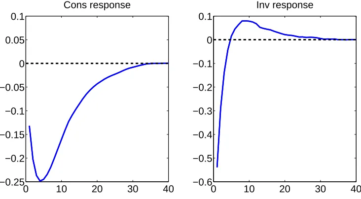
Consider the consumption and investment responses of the agents to a pure downturn risk
and investment decrease, output must decrease as well. This comovement occurs with the
introduction of a moderate amount of habit persistence h = 0.75. The lower productivity
growth expectations lead agents to lower consumption immediately due to the wealth effect.
Because productivity does not change, this usually puts strong upward pressure on
invest-ment from the resource constraint. In this case, investinvest-ment declines due to the expected
increase in the depreciation rate, which lowers the expected return on investment.
Con-sumption habit persistence also helps reduce the immediate incentive to cut conCon-sumption,
as agents do not want to change consumption allocations too quickly, thereby aiding in
generating comovement.
0 10 20 30 40
−0.25 −0.2 −0.15 −0.1 −0.05 0 0.05 0.1
Cons response
0 10 20 30 40
−0.6 −0.5 −0.4 −0.3 −0.2 −0.1 0 0.1
Inv response
Figure 6 Impulse responses of consumption and investment to pure downturn risk shock (multipled by 100 log deviations from steady state)
Figure 7 displays the response of agents to the three 4−period ahead news shocks at the same parameter calibration where appropriate. The blue line gives the response to negative
productivity growth news. Having only consumption habits cannot produce comovement
in response to productivity growth news. Agents, understanding that productivity will
decrease in the future, would like to immediately cut consumption. This leads them to
increase investment. Consumption habits mitigate the incentive to immediately decrease
comovement. Relative to productivity growth news, the downturn risk shock also increases
the expected depreciation rate, thereby reducing the incentive to invest.
The endogenous response to negative MEI news (black line) has the same difficulty in
gener-ating comovement. In this case, agents understand that the future efficiency of investment
will decrease. When the news shock realizes, agents would want to cut investment, thereby
increasing consumption from the resource constraint. Due to habit persistence, they would
not want to change consumption allocations too quickly. Therefore, in response to
expecta-tions of a future decline in MEI, agents decide to immediately begin increasing consumption.
Increased consumption tends to produce decreased investment from the resource constraint,
and the news shock does not lead to comovement.
News about future increases in depreciation (red line) generate an immediate decline in
investment and corresponding increase in consumption. Investment declines because the
knowledge of future depreciation rate increases makes investment today less attractive.
Again, due to the resource constraint holding, decreased investment tends to increase
con-sumption. The downturn risk shock counteracts this issue by having a productivity growth
component. Decreased productivity growth expectations incentivize agents to decrease
0 10 20 30 40 −0.8
−0.6 −0.4 −0.2 0 0.2 0.4 0.6
Cons response
0 10 20 30 40
−2 −1.5 −1 −0.5 0 0.5 1 1.5
Inv response
Prod MEI Dep
Figure 7 Impulse responses of consumption and investment to various negative 1 standard deviation 4−period ahead unrealized news shocks (multipled by 100 log deviations from steady state)
One more important difference in comparing the impulse responses in figures 6 and 7 involves
their dynamics beyond the immediate response. The downturn risk shock does a relatively
good job at producing reasonable consumption and investment dynamics. They tend to
both decline and increase together, which matches the general feature of the business cycle.
This happens because the downturn risk shock simultaneously contains news in both sectors,
so the agents not only want to decrease consumption from productivity growth news, but
they also want to cut investment from depreciation news. The news shocks, on the other
hand, lead to a correlation between consumption and investment of close to −1. In other words, when consumption increases, investment tends to decrease and vice versa.
With further modifications to the model involving stronger adjustment costs, it is of course
possible to produce comovement in response to all three news shocks. The interplay
be-tween productivity growth and depreciation that the downturn risk shock features, however,
1.3.3. Why both productivity growth and depreciation are necessary
Are both productivity growth and depreciation necessary for the downturn risk shock to
produce comovement between consumption and investment without large adjustment costs?
I answer this question by looking at the responses of the economy first shutting down
productivity growth and then removing depreciation, presented in figure 8.
0 10 20 30 40
−0.4 −0.3 −0.2 −0.1 0 0.1
Cons response
0 10 20 30 40
−1.5 −1 −0.5 0 0.5 1 1.5
Inv response
No prod No dep
Figure 8 Impulse responses of consumption and investment to pure downturn risk shock shutting down productivity growth and depreciation (multipled by 100 log deviations from steady state)
With productivity growth shut down, the pure downturn risk shock causes an increase in
consumption and decrease in investment. Agents expect higher depreciation in the future,
which lowers investment. From the resource constraint holding, this leads to an upward
response in consumption. Shutting down depreciation leads to the opposite situation. Now
agents decrease consumption due to expectations of future productivity growth declines,
which leads to an increase in investment. The interplay between the two effects creates the
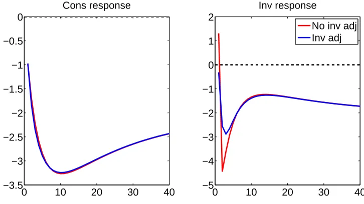
1.3.4. Transition to downturn state
It is important to also analyze the response of the economy to a realization of the downturn
state. The asymmetry of the downturn state generates the negative skewness seen in the
data. As large downward movements in output, consumption, and investment tend to occur
together in the data, it is important to have the proper comovement following a transition
to the downturn state.
0 10 20 30 40
−3.5 −3 −2.5 −2 −1.5 −1 −0.5 0 Cons response
0 10 20 30 40
−5 −4 −3 −2 −1 0 1 2 Inv response
No inv adj Inv adj
Figure 9 Impulse responses of consumption and investment to realization of downturn state with (blue) and without (red) investment adjustment costs (S00= 1) (multipled by 100 log deviations from steady state)
Figure 9 shows the response of the economy with and without a small amount of quadratic
investment adjustment costs14. Investment adjustment costs are just one of many ways
to generate comovement between consumption and investment in response to a realization
of the downturn state. Consumption drops immediately due to the permanent nature of
the productivity decrease. Having a depreciation component incentivizes agents to increase
investment during the period of the transition because they know the capital stock will
14
Investment adjustment costs alter the capital accumulation equation as follows: kt+1 = (1−δt)kt+
1−S00 2
it it−1−e
Λz2
decrease by a large amount in the next period. As the capital stock decreases in the
following period, thereby decreasing output in the economy, investment then drops by a
large amount. Including investment adjustment costs, which penalizes for large movements
in investment, encourages agents to begin decreasing investment the period of the downturn
state transition.
Simulating the economy15in equation 1.3 at the calibrated parameters leads to skewness in
output growth of−0.56, consumption growth of−0.96, and investment growth of−0.23. In contrast, the model with only normally distributed shocks would not produce any skewness
in these variables, and thus could not capture the rapid decreases the model augmented
with downturn shocks can generate.
1.4. Structural estimation
The previous section illustrated the downturn risk shock’s ability to simultaneously capture
the stylized facts in section 2. An important remaining question is the empirical importance
of the downturn risk shock in a larger scale model with competing structural shocks. Are
the properties of the downturn risk shock empirically relevant? I use Bayesian methods
to estimate a dynamic equilibrium model in answering these questions. I first present the
full quantitative model. Then, I lay out the nonstandard model solution method. Third, I
present my estimation algorithm and data. Finally, I discuss empirical results.
1.4.1. Model
I consider a New Keynesian model to conduct my analysis. The model follows the tradition
of Christiano, Eichenbaum, and Evans (2005) and Smets and Wouters (2007). It includes
consumption habits, price, nominal wage, investment, and capacity utilization adjustment
costs, and a Taylor rule that responds to the inflation rate and output growth. Eight