Sparse Coding for Arabic Phoneme Classification

Sparse Coding for Arabic Phoneme

Classification

Dima Shaheen

#1

, Oumayma Al-Dakkak

#2

, MohieldinWianakh

#3

#_{Telecommunication Department, Higher Institute for Applied Sciences and Technology HIAST, Damascus,}

Syria

Abstract—Sparse Coding has been an active research topic in machine learning and signal processing for the last ten years, as it has achieved impressive results when applied to many problems such as face recognition and image denoising. In this paper, we present a new contribution in applying sparse coding to the problem of Arabic phoneme classification. The classification system which is entitled: Sparse Coding based phoneme Classification system (SCPCS), employs the sparse code as a new speech feature for classification using Sparse Representation Classifier. The Sparse code is simply the “coefficients” of the “sparse” (with many zeros) linear combination of basic signals that can represent the targeted signal as close as possible. We study the impact of the sparse coding solver which aims to produce the sparse code, on its discrimination capability. Experiments to evaluate the proposed system performance were conducted on two manually segmented Arabic phonemes, extracted from KAPD (King Abdulaziz city for science and technology Arabic Phonetic Database) and CSLU2002 (Centre for Spoken Language Understanding) Arabic speech databases. Experimental results showed that the proposed system has achieved an accuracy of 85.3% on KAPD and 53.4% on CSLU2002, which are better than state of the art results in these two datasets.

Keywords —Compressive Sensing, Sparse Coding, phoneme classification, dictionary learning, Sparse Representation Classifier SRC, l1 minimization algorithms, cross-validation..

I. INTRODUCTION

For the last 10 years signal model based on sparse representation has been a very active research subject. The interest in sparse representation is motivated by the great success it achieved when applied to many signal processing tasks like image denoising [1], image restoration [2] and super-resolution [3], compressive sensing [4], and blind source separation [5,6]. Sparse coding has been applied also to machine learning tasks, for example it has been used for robust face recognition[7], phoneme classification [8,9,10], and automatic speech recognition [11]. In this paper, we propose to use sparse model for phoneme classification using a

learned dictionary. However, in [8,9] the

classification is done using a dictionary composed of signal exemplars, whereas we investigate the

usefulness of two famous dictionary learning algorithms: K-Singular Value Decomposition (K-SVD) [32] and Fischer Discrimination Dictionary Learning (FDDL) [36] in this context.

The sparse model can be formally defined as follows; let

𝑦 ∈ ℝ

𝑀 be the signal that we’re looking to encode sparsely. We suppose that there is a matrix (Dictionary)

𝐷 ∈ ℝ

𝑀×𝑁 where

𝑀 ≤ 𝑁

such that y can be written as a linear combination of at most k columns of D, where

𝑘 ≪ 𝑁

is called the sparsity degree. The ―sparse coding‖ problem is to find the vector

𝑥 ∈ ℝ

𝑁 that contains only

𝑘

non-zero elements such that:

𝑦 = 𝐷. 𝑥 (1)

The vector x which contains the sparse

coefficients of the linear combination of the elements (called atoms) of the dictionary D, that represents the signal y iscalled the sparse code. As D is over-complete (number of rows is less than the number of columns), this is an ill- posed inverse problem. The theory of Compressive Sensing proves [12] that if D has low coherence(coherence is the maximum correlation between any two dictionary atoms), then solving the following problem gives a unique sparse solution:

𝑃0 𝑚𝑖𝑛

𝑥∈ℝ𝑁 𝑥 ℓ0 𝑠. 𝑡. 𝑦 = 𝐷𝑥 (2)

Where

𝑥

₀ is the l0 pseudo-norm which represents

the number of nonzero elements in x. considering that the signal y might be corrupted with noise, the previous problem has been reformulated as:

𝑃0,𝜖 𝑚𝑖𝑛

𝑥∈ℝ𝑁 𝑥 0 𝑠. 𝑡. 𝑦 − 𝐷𝑥 2≤ 𝜖 (3)

The previous formulation is called the sparse approximation problem. Using the l0 pseudo norm

makes the problem defined by (3) a non-convex optimization problem that has been proved to be an NP-hard [45] (not all nonconvex optimization problems are NP-hard). Relaxing the constraint by using the l1 norm instead of the l0 norm ―convexifys‖

BPDN min

𝑥 ∈ ℝ𝑁 𝑥 1𝑠. 𝑡. 𝑦 − 𝐷. 𝑥 2≤ 𝜖 (4)

Where

𝑥

₁

= 𝑥

𝑁_{1 𝑖} , and

ϵ

is some noise level energy. The previous constrained problem can be reformulated [14] into a problem without constraints using Lagrange Multipliers:

𝐿𝐴𝑆𝑆𝑂 𝑚𝑖𝑛

𝑥 ∈ ℝ𝑁 𝑦 − 𝐷. 𝑥 2+ 𝜆. 𝑥 1 (5)

Where

𝜆 > 0

is a regularization parameter, through which we control the sparsity degree (number of non –zero elements) of the sparse code x. In fact, Tibsherani[14] has proposed the pervious

formulation which he called “Least Absolute

Shrinkage and Selection Operator” (LASSO) to solve the problem of variable selection in classical linear regression.

Algorithms to solve the sparse coding problem (sparse coding solvers) differ in two aspects: The formulation of the problem (mentioned above), and the algorithm used to solve the formulation.

The Sparse Coding consists of two steps: first we should find a dictionary that can represent the signals of interest as a linear combination of a few number of its columns, second we should solve the sparse coding inverse problem to find the sparse code of the signal on the selected dictionary. There are two approaches to tackle the problem of dictionary selection, either we select an off the shelf

dictionary like DCT, wavelets and Gabor

transforms; such dictionaries enjoy both simplicity and fast computation but lack adaptativity to the specific type of signals of interests. In contrast, we can learn an adaptive dictionary from the training signal set. It has been shown that learned dictionary outperforms the non-adaptive ones in many

application like image denoising[1], image

compression [16], and image classification[15,3] .Finding the sparse code over the selected dictionary can be used later as a new feature for discrimination tasks [6-9].

In this paper we propose a sparse coding based phoneme classification system, using supervised discriminative dictionary algorithms to build a compact dictionary, instead of a dictionary composed of signal exemplars [7,8]. Experiments to evaluate the system performance were conducted on two manually segmented Arabic phoneme datasets. Results showed that dictionary learning algorithms do not provide a better classification accuracy over a dictionary composed of signal exemplars, but enable us to have a more ―compact‖ one which makes sparse coding faster. Different sparse coding solvers have been used and demonstrated different discriminative power of the sparse codes.

The paper is organized as follows. In Section 2 we provide a review of the two core problems: sparse coding algorithms and dictionary learning algorithms. In Section 3 the proposed phoneme

classification system based on sparse coding is described. In Section 4 we present the conducted experiments and results. And in Section 5 we summarize and conclude the paper.

II. LITERATURE REVIEW

A. Sparse Coding Solvers

Sparse coding algorithms (solvers) aim to find the sparse representation x of a given signal y on a given dictionary D according to one of the formulations (3),(4) or (5). These algorithms fall into two broad

categories: greedy algorithms, and convex

optimization algorithms. Greedy pursuits algorithms like Orthogonal Matching Pursuits (OMP) [17] and Compressive Sampling Matching Pursuit (CoSaMP) [18] solves (4) iteratively by choosing the best atoms from the dictionary that result in the lowest residual in the sparse approximation of the target signal, and add it to the ―active set‖- the set of dictionary atoms that most resemble the target signal-and re-evaluates the coefficients (sparse code) by solving least-squares on the active set after each round.

Algorithms that adopt the convex l1-norm regularized version of the sparse approximation problem (equation 4 and 5) form another category of sparse solvers. They use convex optimization techniques to solve the sparse coding problem.

Those methods are called l1-minimization

algorithms; because they need to minimize a

function that contains an l1-norm term. l1

minimization algorithms can be classified into: first order methods which use the gradient, second order methods which use the Newton method, and homotopy based methods.

1.First Order Methods: In optimization, first-order methods refer to those algorithms that have at most linear local error, typically based on local linear approximation [20]. Proximity based methods [20] such as FISTA[21] are specifically designed for minimizing nonsmooth functions. They use proximal operator (which is generally the Euclidean Projection) to reformulate the constrained non-smooth problem into multiple smooth sub-problems.

Gradient Projections for Sparse Reconstruction (GPRS) [22] uses a projected gradient descent approach to solve the Lasso problem (5) after splitting x into positive and negative parts to escape the problem with the l1 norm term not being smooth. Other methods such as Spectral Projected Gradient for l1 minimization (SPGL1)[23] uses the projected gradient descent algorithm with a step size specified by Barzilai–Borwein (BB) [23] formulas that select values lying in the spectrum (set of Eigen values) of

𝐷𝑇_{𝐷, which found to provide a good approximation}

for the Hessian.

the constrained problem of sparse coding is reformulated as an Augmented Lagrangian

problem which is divided into three

minimization sub-problems.

The advantage of these first order methods is the low computational complexity per iteration compared to second order methods at the expense of increasing the number of iterations [19].

2. Second Order Methods: which use the Newton Method, such as Primal-Dual Interior Points Algorithm PDIPA [24, 25] and L1LS [27]. PDIPA starts with reformulating the unconstrained

nonsmooth (because of the l1-norm term)

optimization problem (5) into a constrained smooth one, and then it uses the Interior Points method to reformulate this later problem into a nonconstrained smooth optimization problem using the log-barrier. Finally, it employs the Newton method to solve this last one, and thus the worst case complexity of PDIPA is O(n3). L1Ls [27] is an Interior Points method that instead of

using the Newton method which is

computationally expensive, it uses a faster method called the truncated Newton which approximates the Newton system employing the Preconditioned Conjugate Gradient (PCG)[19].

3.Homotopy based method: this is a different type

of l1-miminzation methods which relies on

tracing the solution path in function of the regularization parameter 𝜆 in (5). The name Homotopy reflects the fact the objective function in Lasso (5) experiences a homotopy (continuous deformation) from the l2 objective to l1 objective as 𝜆 decreases. Starting with large 𝜆₀ and construction a decreasing sequence 𝜆𝑘 at which a

change in the ―support set‖ (indexes of the nonzero elements) of optimal solution 𝑥_𝑘∗ takes place, which means either a new nonzero element is added or a previous zero element is removed [47]. The homotopy algorithms runs iteratively, at each iteration it calculates the update direction for only the nonzero element in 𝑥𝑘∗ according to

Newton method. Applying the update direction to

𝑥𝑘∗ may change the ―support set‖, and thus the

update step of 𝑥_𝑘∗is taken as the minimum of magnitude changes in the support set, and the parameter 𝜆𝑘 is lowered by the same magnitude.

The algorithm stops when the difference between two consecutive solutions gets below a desired resolution. Though the Homotopy algorithm uses the Newtonian method, its computational complexity is far beyond the Interior Points method if x is sparse, because the Newtonian system involves only the nonzero elements whose number is small as x is sparse [19]. In our work we have used the greedy OMP. To compare its performance to other l1-minimization algorithms we have used three different first order solvers: GPRS, SPGL1, and DALM. We have also used L1LS which is a second order method and

BPDN-Homopoty[27] which is Homotopy based method.

B. Dictionary Learning

In the classical dictionary learning problem, we seek a matrix D that can represent the training signals yisparsely as close as possible:

𝑚𝑖𝑛

𝐷,𝑋 ( 𝑦𝑖− 𝐷𝑥𝑖 2 2 𝑛

𝑖=1

𝑠. 𝑡. ∀𝑖, 𝑥𝑖 0 ≤ 𝑘 (6)

Where n is the number of training samples (different from N the dimension of x),𝑥𝑖 is the sparse

code vector of the training sample𝑦_i, k is the maximum number of non-zero elements in𝑥𝑖, X is

the matrix composed of all the sparse codes xi.

This optimization problem is nonconvex when both D and X are unknown, however it becomes convex if one of D or X is fixed, that is why it’s generally solved iteratively by fixing the dictionary D and updating the sparse codes X, and then fixing X and updating D.

In fact, dictionary learning is a generalization of the k-means clustering algorithm [29], the only difference is that in k-means each training signal is forced to use only one ―atom‖ from the dictionary (the closest cluster centre) as its representative, while in dictionary learning each signal is allowed to use multiple dictionary atoms provided that it can be approximated by a linear combination of these atoms, and that this linear combination uses as few as possible of the dictionary atoms.

In k-means, we iterate between finding the representative of each training signal (the cluster center which is equivalent to dictionary atom- that minimizes the Euclidean or any other metric distance), and updating the cluster centers; dictionary learning is solved by iterating between two stages [29]. First, the dictionary is fixed and the sparse code𝑥𝑖 for each training signal is calculated

using any sparse coding solver, then the sparse code is fixed and the dictionary atoms are updated to minimize the cost function.

How to update the dictionary atoms is the key difference between dictionary learning algorithms. Some dictionary learning updates the whole set atoms in each iteration. This is the case of one of the early and simple dictionary learning MOD (Method of Optimal Direction) [28], which updates the whole dictionary using the closed form of the Mean Squared Error (MSE) estimator:

𝐷 = 𝑌. 𝑋𝑇_{. (𝑋𝑋}𝑇₎−1 ₍₇₎

OMP to find the sparse code for each training sample. While in the dictionary update stage, for each dictionary atom𝑑_𝑘, K-SVD selects only the training samples that use this atom, which will be denoted asxk, and splits the representation error E into two components: the sparse representation on𝑑𝑘, and the residual error 𝐸𝑘 that accounts for the

sparse presentation error using all the dictionary atoms other than𝑑_𝑘.

𝐸 = 𝑌 − 𝐷𝑋 𝐹 2

= 𝑌 − 𝑑𝑖

𝑁

𝑖=1

𝑥𝑇𝑖

𝐹 2

= 𝑌 − 𝑑𝑖

𝑖≠𝑘

𝑥𝑇𝑖 − 𝑑𝑘𝑥𝑇𝑘

𝐹 2

= 𝐸𝑘− 𝑑𝑘𝑥𝑇𝑘 _𝐹

2

(8)

Where 𝑥𝑇𝑖 represents the sparse coefficients

corresponding to the atom𝑑𝑘, which isith row of the

matrix X (whose columns are the sparse codes for test samples that represent the columns of Y). As the row 𝑥_𝑇𝑘 are all zeros except for the indexes of the test examples in Y that uses the atoms 𝑑_𝑘 , then 𝑑_𝑘𝑥_𝑇𝑘 does not affect the whole 𝐸𝑘, but only affects the

restricted 𝐸_𝑘𝑅 which is composed of the columns of

𝐸𝑘 that correspond to the examples that use 𝑑𝑘.

To update 𝑑𝑘 and 𝑥𝑇𝑘 in a way that minimizes the

restricted error𝐸𝑘𝑅 (which is the only part of the total

error representation E that is affected by the atom

𝑑𝑘), K-SVD evaluates the Singular Value

Decomposition (SVD) for𝐸_𝑘𝑅= 𝑈𝑉𝑇,and updates

𝑑𝑘with the first column of U, while updates the

corresponding sparse coefficients 𝑥𝑇𝑘 as the first

column of V multiplied by  1,1 [29].

The cost function in (6) only measures the representation power of the Dictionary D. In the case of classification task, we are also interested in the discriminative power of the sparse code x. This leads to a new trend in dictionary learning algorithms called ―discriminative‖ or ―supervised‖ dictionary learning in which the cost function reflects both the representation and classification error.Suo [30] has proposed the most general formulation of the discriminative dictionary learning problem as follows:

min

𝐷,𝑋 ( 𝑦𝑖− 𝐷𝑥𝑖 2 2 𝑛

𝑖=1

+ 𝜆1 𝑥𝑖 1 ) + 𝜆2𝑓𝑋 𝑋

+ 𝜆3𝑓𝐷 𝐷 (9)

Where 𝑓_𝑋 𝑋 is a function that measures the discriminative power of the sparse codes X, and

𝑓𝐷 𝐷 is a function that measures the discrimination

power of the atoms of D.

Discriminative Dictionary learning algorithms fall into three categories. In the first category, a shared

dictionary by all classes is learned, while forcing the sparse codes to be discriminative (λ3 = 0), for

example Mairal et al. [31] proposed to add a logistic loss function on the sparse code as a discriminative measure. Zhang et al. proposed Discriminative K-SVD (D-KK-SVD) [32] that adds a linear regression term to learn a linear classifier on the sparse coefficients to the objective function in the Dictionary learning problem formulation (6), as for the case of Label Consistent-KSVD (LC-KSVD) [33] a label consistency term is added that measures how much the sparse codes are consistent with the class labels.

In the second category, only the discriminative power of the dictionary atoms is considered (λ₂=

0), for example Ramirez et al. proposed learning class-specific sub-dictionaries for each class with a structural incoherence penalty term to make the sub-dictionaries as independent as possible [34].

A hybrid discriminative dictionary learning forms the third category where both the dictionary atoms and the sparse codes are forced to be discriminative (λ₂≠ 0, λ₃≠ 0), like the case of COPAR [35] and FDDL[36].

Fischer Discriminative Dictionary Learning

FDDL [36] uses labels information in both the dictionary update stage and the sparse coefficients finding stage. In FDDL, the sparse codes of the training samples are forced to have small within-class scatter but big between-within-class scatter. Also, each class-specific sub-dictionary is forced to have good reconstruction capability for the training samples from that class but poor reconstruction capability for other classes. Therefore, both the representation residual and the sparse coding coefficients of the test sample are discriminative. Thus the optimization problem to learn the dictionary in FDDL is formulated as follows:

min

𝐷,𝑋 𝑟 𝑌, 𝐷, 𝑋 + 𝜆1 𝑋 1 + 𝜆2𝑓𝑋 𝑋

𝑠. 𝑡. 𝑑𝑖 2= 1 , ∀ 𝑖 ∈ {1. . 𝐾} (10)

Where 𝑟 𝑌, 𝐷, 𝑋 is a cost function that measures the discriminative power of the dictionary D, 𝑋 1

is the sparsity penalty term, and 𝑓𝑋 𝑋 is a cost

function that measures the discriminative power of the sparse codes X, 𝐾 is the number of columns of

𝐷.

The cost function that imposes discrimination on the atoms of the dictionary D is defined as follows:

𝑟 𝑌𝑖, 𝐷, 𝑋𝑖 = 𝑌𝑖− 𝐷𝑋𝑖 𝐹 + 𝑌𝑖− 𝐷𝑖𝑋𝑖𝑖 _𝐹

+ 𝐷𝑗𝑋𝑖𝑗 𝐹

2 𝑐

𝑗 =1 𝑗 ≠𝑖

(11)

Where 𝐴 𝐹 = 𝑎𝑖 𝑗 𝑖𝑗2 is the Frobenius norm.

error of samples 𝑌𝑖 (of class i) over the total

dictionary D, the second term represents the representation error of 𝑌𝑖over the i-class specific

sub-dictionary 𝐷𝑖, while the third term represents the

contribution of other subdictionaries than 𝐷𝑖in the

sparse representation of samples 𝑌_𝑖 (which should be small as those samples belong to different class).

The function 𝑓𝑋 𝑋 is a cost function that imposes

discrimination on the sparse codes X according to Fischer Discrimination criterion [36], which means that the sparse codes X should have minimum within-class scatter denoted as𝑆_𝑊 𝑋 , and maximum

between-class scatter denoted as 𝑆𝐵 𝑋 . A

regularization termthat shrinks 𝑋 𝐹2is added to

make 𝑓_𝑋 𝑋 more smooth and convex [37]:

𝑓𝑋 𝑋 = 𝑡𝑟 𝑆𝑊 𝑋 − 𝑡𝑟 𝑆𝐵 𝑋 + 𝜂 𝑋 𝐹2 (12)

Where 𝜂 is a regularization parameter that controls the energy of the samples, tr is the matrix trace operator.

When the labels information are embedded explicitly into the DL problem as in the case of FDDL, Sparse Representation Classifier SRC [7] can be used: It calculates the class-specific residue of the sparse code for the targeted signal, and chooses the class that gives the minimum residue. However, if the labels information are implicitly embedded linear classifier such as SVM can be used.

III.SPARSE CODING BASED PHONEME

CLASSIFICATION SYSTEM (SCPCS)

Sainath et al. were the first to propose employing

Sparse coding for phoneme classification

[9,10].They used the sparse coding of the phoneme test samples, on a dictionary composed of phoneme exemplars as discriminative features, and fed these sparse codes to the Sparse Representation Classifier [7] for classification. Sivaram et al. in [10] proposed employing sparse coding for phoneme recognition. They used the sparse code as a new speech feature to train Multi-Layer Perceptron MLP network to get the posterior probabilities that will be used as emission likelihood of the HMM states. Every phoneme is modelled as a 3 state HMM, and Viterbi decoder is used for phoneme recognition. Our work differs from the previous ones in two aspects; first we consider using dictionary learning algorithms to build a more compact phoneme dictionary, second we are using a ―clipping‖ stage before applying the sparse coding, to make all the segments of the same length.

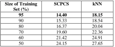
The proposed SCPCS system contains five stages: signal pre-processing, features extraction, feature

clipping, dictionary creation, and phoneme

recognition (figure1). At the pre-processing stage

silence from speech segments are removed, and pre-emphasis filter is applied to cancel lips effect. At the feature extraction stage phoneme speech segments are divided into frames of length 25ms with 10ms overlapping. If the speech segment is shorter than 25 ms, zero padding is applied. After speech framing different well-known speech features are being extracted: Mel Frequency Cepstral Coefficients (MFCC), Relative Spectral Transform - Perceptual Linear Prediction (Rasta-PLP) [38], Sparse Auditory Reproducing Kernel (SPARK) [39], and Gammatone [40]. At the feature clipping stage, feature vectors for each phoneme segment are clipped and a window of only L frames centered at the middle of the phoneme speech is extracted. If the number of feature vectors for the phoneme sample is shorter than L frames, zero padding is applied. The window is reshaped to form one feature vector Vj.

At the dictionary creation stage, the clipped feature vectors of the training phoneme samples are warped together to form one matrix: the initial exemplar dictionary, which is either directly used to find the sparse code for the test samples or fed to the

dictionary learning subsystem. Two famous

dictionary learning algorithm are considered: K-SVD and FDDL.

In the recognition phase, the sparse code of the clipped feature vector for the test sample is calculated using one of the sparse solvers. The sparse code is used by the Sparse Representation Classifier [7] to detect the class to which the corresponding speech segment belongs to.

To solve the equation in step 1, different solvers are used in view of performance comparison: greedy OMP, l1-minimization algorithms: GPRS, SPGL1,

DALM, Homotopy, L1LS. The Matlab

implementations for these methods are available at [26, 27]. To compare with the l2 norm regression, inone experiment we computed x according to the

Mean Squared Error Estimator, instead of l1 lasso regularized problem in step 1.

𝑥 = 𝑎𝑟𝑔𝑚𝑖𝑛

𝑥 𝑦 − 𝐷. 𝑥 2

2_{+ 𝜆. 𝑥}

1

𝑐 = 𝑎𝑟𝑔𝑚𝑖𝑛

𝑖 𝑦 − 𝐷. 𝛿𝑖(𝑥) 2

2_{+ 𝜆. 𝑥}

1

Sparse Representation Classifier SRC

1. Find the sparse code for the clipped feature vector y, by solving Lasso

2. for each sub-dictionary Di of D, find the

energy of the corresponding coefficients in the sparse code x.

3. the class of y, is the index of sub- dictionary whose corresponding sub-sparse code energy is the highest:

Where𝛿𝑖(𝑥)is a selector operator that selects the

0 0.1 0.2 0.3 0.4 0.5 0.6 0.7 -0.4

-0.3 -0.2 -0.1 0 0.1 0.2 0.3 0.4 0.5

0.6 ZULLUZ

Fig 1. Sparse Coding based Phoneme Classification System (SCPCS) detailed block diagram

IV.EXPERIMENTS

A. Phoneme Databases

In 2000, King Abdulaziz City for Science and Technology (KACST) has published a detailed and comprehensive Arabic speech database called KACST Arabic Phonetics Database (KAPD) [41].This database consists of 340 semi-Arabic uttered words that were artificially created and recorded 7 times in different environments by seven male speakers (2380 words). Figure 2 shows an

example of these semi-words, the semi-word 1

―Zalaz‖ in time domain, and its spectrogram with the first four formants.

Nadia and Toni in [43] proposed to segment these semi-words into 33 different phonemes: 28 consonants representing the essential 28 Arabic letters plus 3 phonemes representing the short vowels (a, i, u). In addition, as the letter A in the Arabic language has two different pronunciations, an

1_{These semi-words are in fact ―logatoms‖: artificial}

syllable without meaning.

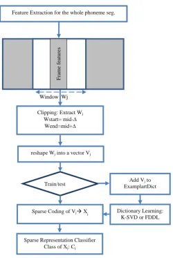
extra phoneme was also used for the long form of letter A to represent this sound. Also, the silence between phonemes and words is represented as a phoneme. Figure 3 [44] shows the 33 different phonemes classified into different acoustic groups. They have manually segmented 2229 phonemes corresponding to the 33 classes, from different semi-words uttered by 4 different speakers. In fact, this classification suffers from some problems: long /u/ and long /i/ are different from the semi vowels /w/ and /y/, the latter are consonants and not taken into consideration. This means the clusters labeled /w/ and /y/ may contain 2 different clusters each. On the other hand, the laterals are only /l/ and /r/ while /j/ and /Z/ are voiced fricatives but this error has no impact on the clustering experiments.

Feature Extraction for the whole phoneme seg.

F

ra

me

f

ea

tu

re

s

Add Vj to

ExamplartDict

Sparse Representation Classifier

Class of Xj: Cj

Window Wj

reshape Wj into a vector Vj

Clipping: Extract Wj

Wstart= mid-

Wend=mid+

Sparse Coding of Vj X_j

Train/test

Fig 2. Semi word ―Zalaz‖ in time domain (top) and the corresponding spectrogram (bottom)

The CSLU speech database contains 22 groups for 22 different languages including Arabic [42]. The Arabic corpus contains continuous and spontaneous telephone speech for 98 callers (70 males, 32 females, 5 children) from 12 different Arab countries (different dialect). Nadia and Toni [43] has chosen 1997 wave files corresponding to 17 male speakers and 17 female speakers, sampled at 8 kHz and digitized using 8 bits per sample. They have manually segmented 3802 phonemes from 33 classes in the frequency domain.

Fig 3. Arabic Phoneme categorization [44]

Fig 4. Segmented speech signals corresponding to phonemes: /ا/, /ب/,/ت/,/ث/ in time domain

B. Experimental Results

As the number of phoneme samples in both datasets is very limited, instead of dividing the dataset into one training set and one test set, we used k-fold cross validation, with different values for k

(5:10), to study the impact of the number of training samples on the recognition accuracy. In k-fold cross validation, the dataset set is randomly divided into k groups of the same size, one group is used for testing, while the other k-1 groups are used for training. Cross-validation is also suitable for tuning the different parameters related to dictionary learning and sparse coding solvers. Experiments are conducted using Matlab 2014Ra, on a desktop PC with 2.13 GHz two processors Intel(R) Xeon(R) CPU, and 8 GB RAM.

For each dataset we have three scenarios: in the first scenario we used the exemplars dictionary directly, in the second one we used the K-SVD dictionary, and in the third we used the FDDL dictionary. In the second scenario, for each class 𝑖 ∈

{1. .33}, training exemplars that belong to this

specific class are passed to the K-SVD dictionary learning algorithm, which has 2 parameters to be tuned: the number of atoms of the dictionary, and the sparsity degree; thus we will have one K-SVD dictionary for each class, and those class-specific dictionaries will be wrapped together to form one whole dictionary to be used by the SRC. In the third scenario all the training exemplars are passed to the discriminative dictionary learning FDDL algorithm, which has three parameters to be tuned: the number of atoms per sub-dictionary Di, 𝜆1 the regularization

parameter that controls the sparsity degree of the sparse codes, and 𝜆2 the regularization parameter

that controls how much Fischer Discrimination is imposed on the sparse codes (equation 10). All the parameters are tuned through cross-validation. Different values for the number of atoms in each class specific sub-dictionary were tried and we found that the optimal value is 25 atoms for FDDL, while it is 20 atoms for K-SVD. In the clipping stage, different values for L (2:6) are considered to find the best clipping length, which we found to be 3 frames.

Table 1 shows the classification error for the three scenarios. We can see that FDDL gives about 6% higher accuracy than the constructive dictionary K-SVD, which is quite logical as the FDDL is designed to be discriminative. When comparing FDDL to plain exemplars dictionary, we found that exemplars dictionary gives about 5% higher due to the fact that phoneme’s samples of the same class have high scatter, and using FDDL which try to minimize the within-class scatter is not a good choice to impose discrimination on such relatively high scattered classes.

Table I. Classification error for different dictionary scenarios using GPRS solver

Phoneme database Dictionary

CSLU2002 KAPD

46.63% 14.40%

Exemplars Dictionary

51.20% 25.74%

K-SVD

48.61% 19.22%

FDDL

0 0.05 0.1 0.15 0.2 -0.4

-0.2 0 0.2 0.4

Aa

0 0.005 0.01 0.015 0.02 -0.1

0 0.1 0.2 0.3

Ba

0 0.01 0.02 0.03 0.04 -0.04

-0.02 0 0.02 0.04

Ta

0 0.02 0.04 0.06 0.08 -0.02

-0.01 0 0.01 0.02

Table 2 shows the average computational time to find the sparse code for each test sample using GPRS solver over the different dictionaries. As one can see FDDL and K-SVD gives faster computation than the exemplars dictionary, this is because the number of atoms in both cases is much smaller (20×33=660 for K-SVD, and 25×33=1050 atoms for FDDL) than the number of atoms of the exemplars dictionary which contains the whole training exemplars (2007 atoms when we used 90% of the whole set for training).

Table II. Average sparse coding time for different dictionary scenarios using GPRS solver

Sparse Coding Time (second) Dictionary

0.29 Exemplars

dictionary

0.09 K-SVD

0.12 FDDL

Table 3 shows the classification error rate using different sparse solvers. Sparse coding solvers have some parameters to set: sparsity regularization parameter which is tuned using cross-validation for every solver, and stopping criterion (the sparse approximation accuracy, the number of elements in the sparse approximation). We used as ―stopping criterion‖ the sparse approximation accuracy which is set for all solvers to 0.001 for a fair comparison. One can see that first order algorithm: GPRS, SPGL1, and DALM give the highest accuracy, while greedy algorithm OMP gives relatively poor performance, and the l2 norm MSE (Mean Squared

Error estimator) gives the worst performance. This proves that the l1 regularization is truly beneficial.

Also we can note the high difference between classification error rate on KAPD dataset (14.73%) and CSLU2002 dataset (46.63%). This is because of the poor quality of the CLSU2002 speech segments, as it contains telephone speech with only 8 KHz sampling frequency, from different Arabic accents, while the KAPD dataset contains speech recorded in a noise free recoding room using 44100 Hz sampling frequency, and all speakers have the same Arabic accent.

Table III. Classification error (%) for different sparse coding solvers using Rasta-PLP features

CSLU2002 (%) KAPD (%)

Method

56.41 20.32

1-NN k-NN

73.14 44.10

L2-MSE

l2 Regression

56.14 20.77

OMP Greedy l0

46.63 14.73

GPSR

First order

l1-minimization SPGL1 14.73 48.19 49.23 16.10

DALM

55.32 20.13

L1LS Second order

l1-minimization

50.18 16.87

BPDN-Homotopy Homotopy

Table 4 shows the average computational time of the sparse coding solvers which we have used in our study. We can see the OMP has the lowest computational time. As for the l1-minimization algorithms, Spectral Projection Gradient for l1 minimization SPGL1 is the fastest. We can see that almost all first order methods are relatively fast with the exception of DALM. The problem with DALM is that it includes three inner minimization sub-problems. We note that GPRS gives also relatively higher computational time due to the fact that the size of the problem is doubled by splitting x into positive and negative parts which make the GPRS complexity 𝑂(𝑁2), while the SPGL1 complexity

𝑂 𝑁𝑀 where 𝑀, 𝑁 are the dimensions of the

dictionary. In our case 𝑀 = 57 (3 frames, each has 19 Rasta-PLP coefficients) and 𝑁 = 2007 (90% of all the 2229 training samples).

Table IV. Sparse coding solvers average time

Time(sec) Coding Method

0.023 MSE

L2 regression

0.0007 OMP

Greedy l0

0.29 GPSR

First order l1 -minimization first

order

0.03 SPGL1

1.03 DALM

1.73 L1LS

Second order l1 -minimization

0.023

BPDN-Homotopy Homotopy

Table 5 shows how using different speech features (MFCC, Rasta-PLP, SPARK, Gammatone) affects classification accuracy. As we can see the Rasta-PLP of order 18 gives the highest accuracy.

Table V. Classification error (%) for different speech features, for the two dataset KAPD and CSLU2002.

Features KAPD CSLU2002

MFCC 17.20 52.23

RASTA-PLP 14.73 46.63

Gammaton 20.10 54.10

SPARK 19.31 53.31

Table VI. Classification error (%) for the proposed SCPCS and kNN vs different percentage of training set size out of the whole

dataset

Size of Training Set (%)

SCPCS kNN

95 14.40 18.15

90 15.33 18.54

80 16.37 20.04

70 19.60 22.36

60 21.42 24.91

50 24.15 27.65

Figure 5 shows the classification error for each phoneme. As we can see, plosive phonemes such as /ba/,/ta/ have high misclassification rate, as they are generally hard to recognize. Also the unvoiced fricative /fa/ has the highest misclassification, as the number of available training samples is low (only 47 samples for phoneme /fa/ while the mean of the training samples per phoneme is 61), and it is confused with the fricative phoneme /th/. The vowel /Aa/ also has a high misclassification rate and it is only confused with the short vowel /a/ (Fatha). The voiced phoneme /Da/ ض and the vowel /wa/ have the lowest classification error. The phoneme / Da /was confused with only one phoneme which is /Ha/ ح, and also /wa/ was confused with only one phoneme which the short vowel /u/ (Damah). The vowel /ya/ ي was only confused with the short vowel /i/ (Kasra). While the short vowel /i/ was confused with three phonemes: /ya/, /ha/ and /ba/, because the speech segments for these phonemes include in part the sound of the short vowel /i/. This means that we need a better dictionary that can represent multi-scale information.

Figure 6 shows the classification error as a function of number of training samples for each phoneme (as we have different number of samples per class according to the dataset we had from Nadia [43]), and it is clear that classification error decreases in general, as the number of training samples in each class increases.

Fig 5. Phoneme classification error.

Fig 6. Phoneme misclassification error vs number of trainingexemplars for KAPD dataset

V. CONCLUSION

In this paper a sparse coding based phoneme

recognition system is proposed.The system

performance has been evaluated using two Arabic phoneme databases. Experimental Results prove that the proposed system outperforms state of the art results in the studied dataset with accuracy 85.3% on KAPD dataset and 53.4% on CSLU2002 dataset, while the accuracy achieved using Echo State Neural Networks is 72.31 % and 38.2% respectively [43].

We have found that choosing the sparse coding solver affects the recognition accuracy; greedy solver gives relatively lower classification accuracy though they are very fast, while first order solvers like GPRS and SPGL1 gives the highest accuracy, with low computational complexity. We found that Spectral Projected Gradient for l1 minimization (SPGL1) is the most suitable sparse coding algorithm in the context of phoneme classification, as opposed to DALM in the context of face recognition [19], as it gives the highest accuracy with minimum computational time. Also we have found that the best value for the sparsity regularization parameter (𝜆) is the same for the two datasets.

Comparing different scenarios for dictionary learning, we have found that using a discriminative dictionary learning algorithm does not enhance the classification accuracy because the speech samples of specific phoneme have high within-class scatter, so Fischer criterion to decrease inter-class scatter is not a good scheme to increase the discrimination of the sparse code. We have found that the only advantage of using learned dictionaries in the context of phoneme classification is the lower computational time of the sparse code as the dictionary become more compact.

Different well-known speech features were compared, and we found that Rasta-PLP of order 18 provides the best accuracy, with 2% higher accuracy than the famous MFCC features.

Finally, we have found that the number of training samples affects the discriminative ability of the exemplars dictionary, and increasing the number %0^ Aa batavajaHa xada!arazasa$a Sa Da TaZaEa gafaqakalama naha wa yaa i u 0

0.05 0.1 0.15 0.2 0.25 0.3 0.35 0.4 0.45

of atoms for each exemplars sub-dictionary enhance the discriminative power of this dictionary, while increasing the number of atoms for the learned K-SVD and FDDL dictionary over a specific optimal value tuned through cross validation decreases the classification accuracy. This is due to that fact that in both dictionary learning algorithms we are learning from a specific training set with a fixed size, so we can capture all the information using an optimal value of atoms, and increasing the number of atoms to represent this specific training set will only include more redundancy that increases the ―coherence‖ of the dictionary, which has been proven to produce poor sparse approximation [46]. While increasing the size of the training set in

learning K-SVD and FDDL improves the

classification accuracy for a specific optimal number of atoms.

Further works regarding the relation between the

sparse coding approximation accuracy and

classification accuracy, and how to build a compact discriminative dictionary more suitable for the specific case of speech data needs to be addressed in future; especially, after validation of the datasets segmentation by linguistic experts.

References

[1] M. Elad and M. Aharon, ―Image denoising via sparse and redundant representations over learned dictionaries,‖

IEEE Trans. Image Process., vol. 15, no. 12, pp. 3736-3745, Dec. 2006.

[2] J. Mairal, M. Elad, and G. Sapiro, ―Sparse representation for color image restoration,‖ IEEE Trans. Image Process., vol. 17, no. 1, pp. 53-69, Jan. 2008.

[3] M. Elad, M. A. T. Figueiredo, and Y. Ma, ―On the role of sparse and redundant representations in image processing,‖ Proceedings of the IEEE, vol. 98, no. 6, pp. 972–982, 2010.

[4] D. L. Donoho, ―Compressed sensing,‖ IEEE Trans. on Information Theory, vol. 52, no. 4, pp. 1289–1306, April 2006.

[5] M. G. Jafari, Samer A., Mark D., Mike E., ―Sparse Coding for Convolutive Blind Audio Source Separation‖, Book Section, ―Independent Component Analysis and Blind Signal Separation‖ Lecture Notes in Computer Science ISBN 978-3-540-32630-4, Springer Berlin Heidelberg ,2006, P 132-139

[6] X. Zhao, G. Zhou,W. Dai, W. Wang, ―Blind Source Separation Based on Dictionary Learning: A Singularity-Aware Approach‖ Book Section ―Blind Source Separation‖ ISBN 978-3-642-55015-7, Springer Berlin Heidelberg,2014, P 39-59

[7] Wright J, Yang A, Ganesh A, Sastry SS, Ma Y (2009), ―Robust face recognition via sparse representation‖. IEEE Trans Pattern Anal Mach Intell 31: 210–227

[8] Sainath, T.N., Kanevsky, D, ―Sparse Representations for Speech Recognition‖, Book Section ―Compressed Sensing & Sparse Filtering” Springer Berlin Heidelberg 2014, P 455-502

[9] Sainath, T.N.; Carmi, A.; Kanevsky, D.; Ramabhadran, B., "Bayesian compressive sensing for phonetic classification", Acoustics Speech and Signal Processing (ICASSP), 2010 IEEE International Conference on , vol., no., pp.4370,4373, 14-19 March 2010

[10] Sivaram, G.S.V.S.; Nemala, S.K.; Elhilali, M.; Tran, T.D.; Hermansky, H., "Sparse coding for speech recognition,"

in Acoustics Speech and Signal Processing (ICASSP),

2010 IEEE International Conference on, vol., no., pp.4346-4349, 14-19 March 2010

[11] Gemmeke, J.F.; Virtanen, T.; Hurmalainen, A., "Exemplar-Based Sparse Representations for Noise Robust Automatic Speech Recognition," in Audio, Speech, and Language Processing, IEEE Transactions on,

vol.19, no.7, pp.2067-2080, Sept. 2011

[12] E. J. Candes and M. B. Wakin, "An Introduction to Compressive Sampling," in IEEE Signal Processing Magazine, vol. 25, no. 2, pp. 21-30, March 2008 [13] S. S. Chen, D. L. Donoho, and M. A. Saunders, ―Atomic

decomposition by basis pursuit,‖ SIAM Journal on Scientific Computing, vol. 20, no. 1, pp. 33–61, 1999 [14] Tibshirani, R. (2011), ―Regression shrinkage and

selection via the lasso: a retrospective‖. Journal of the Royal Statistical Society: Series B (Statistical Methodology), 73: 273–282. doi:10.1111/j.1467-9868.2011.00771.

[15] J. Mairal, F. Bach and J. Ponce, "Task-Driven Dictionary Learning," in IEEE Transactions on Pattern Analysis and Machine Intelligence, vol. 34, no. 4, pp. 791-804, April 2012.

[16] O. Bryt and M. Elad, ―Compression of facial images using the K-SVD algorithm,‖ Journal of Visual Communication and Image Representation, vol. 19, no. 4, pp. 270–283, 2008.

[17] Y. C. Pati, R. Rezaiifar, and P. S. Krishnaprasad, ―Orthogonal matching pursuit: recursive function approximation with applications to wavelet decomposition,‖ In Proc. Asilomar Conf. Signal Syst. Comput., 1993.

[18] D. Needell and J. A. Tropp,―CoSaMP: Iterative signal recovery from incomplete and inaccurate samples,‖ Appl. Comput. Harmon. Anal.,vol. 26, no. 3, pp. 301_321, 2009. [19] A. Y. Yang, Z. Zhou, A. G. Balasubramanian, S. S. Sastry and Y. Ma, "Fast l1-Minimization Algorithms for Robust

Face Recognition," in IEEE Transactions on Image Processing, vol. 22, no. 8, pp. 3234-3246, Aug. 2013. [20] Z. Zhang, Y. Xu, J. Yang, X. Li and D. Zhang, "A Survey

of Sparse Representation: Algorithms and Applications," in IEEE Access, vol. 3, no., pp. 490-530, 2015

[21] A. Beck and M. Teboulle, ―A fast iterative shrinkage-thresholding algorithm for linear inverse problems,‖ SIAM J. Imag. Sci., vol. 2, no. 1, pp. 183_202, 2009.

[22] M. A. T. Figueiredo, R. D. Nowak, and S. J. Wright, ―Gradient projection for sparse reconstruction: Application to compressed sensing and other inverse problems,‖ IEEE J. Sel. Topics Signal Process., vol. 1, no. 4, pp. 586_597, Dec. 2007.

[23] E. G. Birgin, J. M. Martınez and M. Raydan, ―Nonmonotone spectral projected gradient methods on convex sets,‖ SIAM Journal on Optimization, 10, pp. 1196–1211, 2000.

[24] J. A. Tropp and S. J. Wright, ―Computational methods for sparse solution of linear inverse problems,‖ Proceedings of the IEEE, vol.98, no. 6, pp. 948–958, 2010.

[25] S.-J. Kim, K. Koh, M. Lustig, S. Boyd, and D. Gorinevsky, ―An interior point method for large-scale l1

regularized least squares,‖ IEEE J. Sel. Topics Signal Process., vol. 1, no. 4, pp. 606_617, Dec. 2007.

[26] SPGL1: A solver for large-scale sparse reconstruction: https://www.math.ucdavis.edu/~mpf/spgl1/

[27] l1 benchmark

https://people.eecs.berkeley.edu/~yang/software/l1bench mark/

[28] K. Engan, S. O. Aase, and J. HakonHusoy, ―Method of optimal directions for frame design,‖ in Proceedings of IEEE ICASSP, 1999, vol. 5

[29] M. Aharon, M. Elad, and A. Bruckstein, ―K-SVD: An algorithm for designing overcomplete dictionaries for sparse representation,‖ IEEE Trans. on Signal Processing,

vol. 54, no. 11, pp. 4311–4322, 2006.

[31] J. Mairal, F. Bach, J. Ponce, G. Sapiro, A. Zisserman, ―Supervised dictionary learning,‖ Advances in Neural Information Processing Systems (NIPS), MIT Press, 2008, pp. 1033–1040.

[32] Q. Zhang and B. Li, ―Discriminative K-SVD for dictionary learning in face recognition,‖ in Proc. IEEE Conf. Comput. Vis. Pattern Recognit., Jun. 2010, pp. 2691-2698.

[33] Z. Jiang, Z. Lin, and L. S. Davis, ―Label consistent K-SVD: Learning a discriminative dictionary for recognition,‖ IEEE Trans. Pattern Anal. Mach. Intell., vol. 35, no. 11, pp. 2651-2664, Nov. 2013.

[34] I. Ramirez, P. Sprechmann, G. Sapiro, ―Classification and clustering via dictionary learning with structured incoherence and shared features‖, CVPR, IEEE, 2010, pp. 3501–3508.

[35] S. Kong and D. Wang, ―A dictionary learning approach for classification: Separating the particularity and the commonality,‖ in Proc. 12th Eur. Conf. Comput. Vis. (ECCV), 2012, pp. 186-199.

[36] M. Yang, L. Zhang, X. Feng, and D. Zhang, ―Fisher discrimination dictionary learning for sparse representation,‖ in Proc. IEEE Int. Conf. Comput. Vis.,

Nov. 2011, pp. 543_550. Jun. 2010, pp. 2691-2698. [37] Meng Yang, Lei Zhang, Xiangchu Feng, ―Sparse

Representation Based Fisher Discrimination Dictionary Learning for Image Classification,‖International Journal of Computer Vision, 2014.

[38] H. Hermansky and N. Morgan, "RASTA processing of speech", IEEE Trans. on Speech and Audio Proc., vol. 2, no. 4, pp. 578-589, Oct. 1994.

[39] A. Fazel and S. Chakrabartty, "Sparse Auditory Reproducing Kernel (SPARK) Features for Noise-Robust Speech Recognition," in IEEE Transactions on Audio, Speech, and Language Processing, vol. 20, no. 4, pp. 1362-1371, May 2012.

[40] Hui Yin, Volker Hohmann, ClimentNadeu, ―Acoustic features for speech recognition based on Gammatonefilterbank and instantaneous frequency‖,

Speech Communication, Volume 53, Issue 5, May–June 2011, Pages 707-715, ISSN 0167-6393,

[41] KAPD: KACST Arabic Phonetics Database https://sourceforge.net/projects/kapd/ [42] CSLU2002

http://www.cslu.ogi.edu/corpora/22lang/

[43] HMAD, N. and ALLEN, T., 2013. ―Echo State Networks for Arabic phoneme classification and recognition.‖ 34th International Conference on Machine Learning and Pattern Recognition (ICMLPR 2013), Venice, Italy, 14-15 November 2013. Venice, Italy.

[44] HMAD, N. and ALLEN, T.J., 2012. ―Biologically inspired continuous Arabic speech recognition.‖ Research and development in intelligent systems XXIX. In: M. BRAMER and M. PETRIDIS, eds., Research and development in intelligent systems XXIX. London: Springer, pp. 245-258. ISBN 9781447147381

[45] B. K. Natarajan, ―Sparse approximate solutions to linear systems‖, SIAM Journal on Computing, 24(1995), 227-234.

[46] J. A. Tropp, "Greed is good: algorithmic results for sparse approximation," in IEEE Transactions on Information Theory, vol. 50, no. 10, pp. 2231-2242, Oct. 2004.

[47] A. Y. Yang, A. Ganesh, Z. Zhou, S. S. Sastry, and Y. Ma, ―A Review of Fast l1-Minimization Algorithms for Robust Face