Published online August 30, 2014 (http://www.sciencepublishinggroup.com/j/ajam) doi: 10.11648/j.ajam.20140204.13
ISSN: 2330-0043 (Print); ISSN: 2330-006X (Online)
On generalized fuzzy mean code word lengths
Dhara Singh Hooda, Arunodaya Raj Mishra, Divya Jain
Department of Mathematics, Jaypee University of Engineering and Technology, Guna, Madhya Pradesh, India
Email address:
[email protected] (D. S. Hooda), [email protected] (A. R. Mishra), [email protected] (D. Jain)
To cite this article:
Dhara Singh Hooda, Arunodaya Raj Mishra, Divya Jain. On Generalized Fuzzy Mean Code Word Lengths. American Journal of Applied Mathematics. Vol. 2, No. 4, 2014, pp. 127-134. doi: 10.11648/j.ajam.20140204.13
Abstract:
In present communication, a generalized fuzzy mean code word length of degree β has been defined and its bounds in the term of generalized fuzzy information measure have been studied. Further we have defined the fuzzy meancode word length of type α, β and its bounds have also been studied. Monotonic behavior of these fuzzy mean code word
lengths have been illustrated graphically by taking some empirical data.
Keywords:
Entropy, Fuzzy Entropy, Codeword Length, Decipherable Code, Crisp Set, Hölder’s Inequality1. Introduction
Let X be a discrete random variable with probability
distribution
{
( , , ..., ) : 0; 1}
1 2 1
n
P p p pn pi pi
i
= ≥ ∑ =
= in an
experiment. [5] gave a mathematical formulation to measure uncertainty of the randomness in a probability distribution and information contained in an experiment as
( ) log ,
1
n
H P pi pi i
= −∑
= (1)
which is called Shannon’s entropy.
In many applications of the uncertainty function, the main problem generated by researchers is that of efficient coding of message to be sent over a noiseless channel, and to maximize the number of messages that can be sent over the channel in a given time. Let us consider that the messages to be transmitted are generated by a random variable
{ 1, 2, ..., }
X = x x x n with the probability distribution
1 2
1
( , ,..., ) : 0; 1 .
n
n i i
i
P p p p p p
=
= ≥ =
∑
Each
x
i is calledsource symbol or alphabet and is represented by a finite
sequence of symbols select from the set
{
1, 2, ...,}
.A= a a a D The set A is known as code alphabet
or set of code characters and the sequence assigned to each
; 1, 2, ...,
i
x i = n is called code word. The number of code
character used for a code word is called code word length.
Let
n
i be the code word length ofx
i, then mean codeword length is given
1
, n
i i i
L p n
=
=
∑
(2)where pi is the probability of occurrence of
x
i satisfyingKraft’s inequality
1
1,
i
n n i
D−
=
≤
∑
(3)where is the size of code alphabet.
In evaluating long run efficiency of communications, we choose codes to minimize average code word length (2).
For uniquely decipherable codes, [5] noiseless coding theorem states that
( ) ( )
1,
log log
H P H P
L
D ≤ ≤ D + (4)
which determines the lower and upper bounds on
L
interms of [5] entropy.
To prove noiseless coding theorem, [11] inequality plays an important role and is uniquely determined by the condition for uniquely decipherability. To tackle such situations, instead of taking the probability, the idea of fuzziness can be explored.
[10] Introduced the concept of fuzzy set in which imprecise knowledge can be used to define an event.
Because of their capability to model non-statistical
imprecision fuzzy set plays an important role in many
( )
( )
[ ]
{
( i A i ) : A i 0,1 ; i}
A= x, µ x µ x ∈ ∀ ∈x X ,
where µA( )xi represents the degree of membership and is
defined as
( )
1, if0, if andthereisnoambiguityandthereisnoambiguity0.5,thereismaximumambiguity whether or xi A
xi xi A
A
xi A xi A ∉
µ = ∈
∉ ∈
The idea of measuring fuzzy uncertainty without reference to probabilities began in 1972 with the work of [1]
who defined the entropy of
A P X
∈
n( )
using Shannon’sentropy as
[ ]
1
( ) ( ) log ( ) (1 ( )) log(1 ( ))
=
= −
∑
n A i A i + − A i − A ii
H A µ x µ x µ x µ x (5)
This is called fuzzy information measure. The fuzzy information measure has found wide applications to Engineering, Fuzzy traffic control, Fuzzy aircraft control, Computer sciences, management and Decision making, etc. and those have already been studied by various authors. [6]
Introduced anew measure of fuzzy divergence explaining its
application to clustering problems and to an object extraction problem.
In present paper, we define fuzzy mean code word lengths in section 2. In section 3, we also study the bounds of the
generalized fuzzy mean code word length of degree β in
terms of fuzzy information measure and we study the bounds of the new fuzzy mean code word length of type
(α β, ) in terms of fuzzy information measure in section 4.
We discuss the monotonic behavior of generalized fuzzy mean code word lengths in section 5.
2. Fuzzy Mean Code Word Lengths
[12] defined fuzzy mean code word length as given below:
(1 ( ))
( )
log 1 .
1
xi A ni
ni Axi D
L D n n
j D j
µ µ
− − −
= − −
∑
=
(6)
They studied the lower and upper bounds of
L
in term of(5).
Further based on [2], they generalized (6) as given below:
{
( ) (1 ( ))}
log ; 0, 1,
1 1
ni
x x D
n A i A i
L i
α
α α
α µ µ
α α
α
α
−
− + −
= ∑ > ≠
= −
(7)
which was called fuzzy mean code word length of order
α
.Its lower and upper bounds were obtained in term of the following fuzzy information measure characterized by [6]:
1
( ) log ( ) (1 ( )) ; 0, 1.
1 1
n
H A xi xi
A A
i
α α
µ µ α α
α = −α ∑=
+ −
> ≠ (8)[12] also defined fuzzy mean code word length of degree β
as given below:
{
}
11
( ) (1 ( )) 1 ; 0, 1, 1
1
n
n i
L A xi Axi D
i
β
β µβ µ β β β β
β
−
= ∑ + − − > ≠
= −
(9)
which was called fuzzy mean code word length of degree
β and studied its lower and upper bounds in term of fuzzy
information defined by [9] and is given as
1
( ) ( ) (1 ( )) 1 ; 0, 1.
1 1
n
H A A xi Axi i
β µβ µ β β β
β
= ∑ + − − > ≠
= −
(10)
Corresponding to [3], [8] proposed and studied the
measure of fuzzy entropy as given below:
{
}
( 1) ( )log ( ) (1 ( ))log(1 ( ))
1 1
( ) 2 1 ,
1
n
xi xi xi xi
A A A A
i
H A
β µ µ µ µ
β β
− ∑ + − −
=
= −
−
where
0, 1.
β > β ≠ (11)
Corresponding to [4], [7] studied generalized sub additive
fuzzy information of type ( , )α β given by
1
( ) 1 1 ( ) (1 ( )) ( ) (1 ( )) , 1
2 2
n
H A Axi Axi A xi Axi
i
β µα µ α µβ µ β
α = −α− −β ∑= + − − − − (12)
where
0< <α 1,β≥1 or 0<β <1,α≥1.
3. Bounds of a Generalized Fuzzy Mean
Code Word Length of Degree
β
It may be noted that (6) can be generalized in various ways; however, we consider the following generalization:
(1 ( )) ( )
(1 ) log 1
1
1 1
2 1 ;
1
xi A n n Dni Axi nD in
j
i D
j L
µ µ
β β
β
− − −
− ∑ − −
= ∑
=
= −
−
(13)
where β >0,β ≠1
and study its bounds in terms of (11).
Theorem 1. For all uniquely decipherable codes, noiseless coding theorem states:
(1 ) 1 (1 )
( ) ( )2 (1 ) (2 1),
Hβ A ≤Lβ ≤Hβ A −β + −β − −β − (14)
( ) , 1
ni D
xi n
A n j
D j µ − = − ∑ =
where Hβ( )A is given by (11).
Proof. [7] have given the following expression for directed divergence:
( ) ( ) log
( )
( 1) (1 ( ))
1 (1 ( ))log
(1 ( )) 1
( , ) 2 1 0
1
xi A xi A
n B xi
xi
i xi A
A xi
B I A B
µ µ µ β µ µ µ β β − ∑ − = + − − = − ≥ − (15)
( )log ( ) ( )log ( ) (1 ( )) ( 1)
log(1 ( )) (1 ( ))log(1 ( )) 1
1
( , ) 2 1 0.
1
x x x x x
n A i A i A i B i A i
x x x
i A i A i B i
I A B
µ µ µ µ µ β µ µ µ β β − + − − ∑ × − − − − = = − ≥ −
Taking ( ) ,1 ,
1
ni D
xi n i n
B n j
D j µ − = − ≤ ≤ ∑ =
( )log ( ) ( )log (1 ( )) 1
( 1) 1
log(1 ( )) (1 ( ))log 1 1 1
( , ) 2 1 0,
1
ni D
xi xi xi n xi
A A A D nj A
j n
i ni
D xi xi n
A A Dnj
j I A B
µ µ µ µ β µ µ β β − − − + − ∑ = − ∑ = − × − − − − − ∑ = = − ≥ −
( ) log log
1 (1 )
1
(1 ( ))log 1 1 1
( ) 2 1 .
1
n
ni n j
xi D D
A j
n
n
i x D i
n i
A D n j
j H A µ β µ β β − − − − ∑ = − ∑ − = − − − − ∑ = ≤ − − (16)
Using Kraft’s inequality, that is
1 1, − = ≤
∑
j n n jD we get
(1 ( )) ( )
(1 ) log 1
1
1 1
( ) 2 1
1
xi A n
n Dni Axi nD i n j i D j H A µ µ β β β − − − − ∑ − − = ∑ = ≤ − − ( ) .
Hβ A ≤Lβ
For uniquely decipherable code, [5] noiseless coding theorem for fuzzy information measure as
( ) ( ) 1.
H A ≤ ≤L H A +
Then we have
( ) 1
L≤H A + .
It implies
(1 ( )) ( )
log 1
1 1
( ) log ( ) (1 ( )) log(1 ( )) 1 1
xi A ni
ni Axi D
D n n
n j
D j i
n
xi xi xi xi
A A A A
i µ µ µ µ µ µ − − − − − ∑ ∑ = = ≤ −∑ + − − + =
(1 ( )) ( )
(1 ) log 1
1
1
( 1) ( ) log ( ) (1 ( )) log(1 ( )) (1 ). 1
xi A ni
n ni Axi D
D n n
j
i D
j n
xi xi xi xi
A A A A
i µ µ β β µ µ µ µ β − − − − ∑ − − = ∑ = ≤ − ∑ + − − + − = It implies
(1 ( )) ( )
(1 ) log 1
1
1
2 1
( 1) ( )log ( ) (1 ( ))log(1 ( )) (1 ) 1
2 1
xi A n
n Dni Axi D i n n j
i D
j
n
xi xi xi xi
A A A A
(1 ( ))
( ) (1 ) log 1
1
1 1
2 1
1
( 1) ( )log ( ) (1 ( ))log(1 ( )) (1 )
1 1
2 1
1
xi A n n Dni Axi nD in
j
i D
j
n
xi xi xi xi
A A A A
i
µ µ
β
β
β µ µ µ µ β
β
− − −
− ∑ − −
= ∑
=
− −
− ∑ + − − + −
=
≤ −
−
{
}
( 1) ( )log ( ) (1 ( ))log(1 ( )) 1
2 1
1 1
(1 ) (1 )
2 2 1
n
xi xi xi xi
A A A A
i
L
β µ µ µ µ
β β
β β
− ∑ + − −
= −
≤ −
− −
× + −
{
}
( 1) ( )log ( ) (1 ( ))log(1 ( ))
1 2 1 1 2(1 )
1
1 (1 )
2 1
1
n
xi xi xi xi
A A A A
i L
β µ µ µ µ
β β
β
β β
− ∑ + − −
− =
≤ −
−
−
+ −
−
(1 ) 1 (1 ) ( ) 2 (1 ) (2 1).
Lβ ≤Hβ A −β + −β − −β −
Hence
(1 ) 1 (1 ) ( ) ( ) 2 (1 ) (2 1).
Hβ A ≤Lβ ≤Hβ A −β + −β − −β −
Particular Case
When β →1, Lβreduces to (6).
(1 ( )) ( )
log 1
1
1
.
xi A ni
n ni Axi D
L D n
nj
i D
j
µ µ
− − −
= ∑ −
−
= ∑
=
Thus (13) can be called the generalized fuzzy mean code
word length of degreeβ .
4. Bounds of Fuzzy Mean Code Word
Length of Type
( , )
α β
In this section, we defined fuzzy mean code word length of type ( , )α β .
{
}
1{
}
11
( ) (1 ( )) ( ) (1 ( )) 1
1 1
2 2
n n
n i i
L Axi Axi D Axi Axi D i
β α
β µα µ α α µβ µ β β
α α β
− −
= − − ∑ + − − + −
= −
where 0<α <1,β ≥1 or 0<β <1,α ≥1. (17)
Theorem 2. For all uniquely decipherable codes, noiseless coding theorem states:
1 1
1
( ) 1
1
2 2
H A L H D D
β α
β α β
β α β
α α α β
− −
≤ ≤ + − −
− −
(18)
where Hαβ( )A is given by (12).
Proof. By Hölder’s inequality, we have
( ) ( )
1 1; 0 1, 0 or 0 1, 0,
1 1 1
n n p p n q q
x yi i xi yi p q q p
i∑= ≥ i∑= i∑= < < < < < < (19)
and
( ) ( )
1 1 1 1; 1, 1, 1and , 0.
1 1 1
n n p p n q q
x yi i xi yi p q x yi i i ≤ i i p+ =q ≥ > >
∑ ∑ ∑
= = = (20)
From (19), we have
( ) ( )
1 1; 0 1, 0 or 0 1, 0.
1 1 1
n n p p n q q
x yi i xi yi p q q p i ≥ i i < < < < < <
∑ ∑ ∑
= = =
Set
1 1
( ( ), ( )) , ( ( ), ( )) and , .
1
ni t
t t
xi f A xi B xi D yi f A xi B xi p t q
t
µ µ − − µ µ
= = = − =
+
Then
1 1
( ( ), ( )) ( ( ), ( ))
1 1 1
n ni n n ti t n t
D f A xi B xi D f A xi B xi
i i µ µ i µ µ
− −
≥
∑ ∑ ∑
= = =
by Kraft’s inequality
1 1
( ( ), ( )) ( ( ), ( )) 1
1 1 1
n n ti t n t n ni
f A xi B xi D f A xi B xi D
i µ µ i µ µ i
−
−
≤ ≤
∑ ∑ ∑
= = =
or
( ( ), ( )) ( ( ), ( )) .
1 1
n n n ti
f A xi B xi f A xi B xi D
i µ µ ≤ i µ µ
∑ ∑
= =
Subtracting n from both sides, we get
{
( ( ), ( )) 1}
{
( ( ), ( )) 1 .}
1 1
n n n ti
f A xi B xi f A xi B xi D
i µ µ − ≤i µ µ −
∑ ∑
= =
Setting 1 , 0, 1
1
t t
α
α α
α
− = > =
+ and
(
A( ),
i B( ))
i A( ) (1
i A( )) .
if
µ
x
µ
x
=
µ
αx
+ −
µ
x
α1
( ) (1 ( )) 1
1
1 1
2 2
1 1
( ) (1 ( )) 1 .
1
1 1
2 2
n
xi xi
A A
i
n
n i
xi xi D
A A i α α µ µ β α α α α α µ µ β α + − − ∑ − − − = − ≤ ∑ + − − − − − = (21)
Changing
α
toβ
, we get1
( ) (1 ( )) 1
1 1 1
2 2
1 1
( ) (1 ( )) 1 .
1 1 1
2 2
n
xi xi
A A
i
n
n i
xi xi D
A A i β β µ µ β α β β β β µ µ β α + − − ∑ − − − = − ≤ − ∑ + − − − = − (22)
Adding (21) and (22), we get
{
}
{
}
1
( ) (1 ( )) ( ) (1 ( )) 1 1 1 2 2 1 1 1
( ) (1 ( )) ( ) (1 ( ))
1
1 1
2 2
n
xi xi xi xi
A A A A
i
n n
n i i
xi xi D xi xi D
A A A A
i β β α α µ µ µ µ β α β α α β β β α α µ µ µ µ β α + − − + − ∑ − − − = − − ≤ − − ∑ + − − + − = −
{
}
{
}
1( ) (1 ( )) ( ) (1 ( )) 1 1 1 2 2 1 1 1
( ) (1 ( )) ( ) (1 ( )) . 1
1 1
2 2
n
xi xi xi xi
A A A A
i
n n
n i i
xi xi D xi xi D
A A A A
i β β α α µ µ µ µ β α β α α β β β α α µ µ µ µ β α + − − − − ∑ − − − = − − ≤ − ∑ + − − + − − − =
Hence H
α
β
( )A ≤Lα
β
. Now, we have to prove1 1 1 1 1 2 2
L H D D
β α β β α β α α α β − − ≤ + − − − − (23) 1 1
( ) 1
1
L H A D
α α α α α − ≤ + − − (24)
{
}
11
( ) (1 ( )) 1
1 1
1
1 1
( ) (1 ( )) 1 1 .
1
1 1
n
n i
xi xi D
A A
i
n
xi xi D
A A i α α α α µ µ α α α α α µ µ α α − + − − ∑ = − − ≤ ∑ + − − + − = − − It implies
{
( ) (1 ( ))}
1 11
1
( ) (1 ( )) 1 1 .
1
n
n i
xi xi D
A A
i
n
xi xi D
A A i α α α α µ µ α α α α µ µ − + − − ∑ = − ≤ ∑ + − − + − = (25)
Similarly, we can prove that
1 1
( ) 1
1
L H A D
β β β β β − ≤ + − −
. (26)
It implies
{
}
11
1
1
( ) (1 ( )) 1
( ) (1 ( )) 1 1 .
i
n n
A i A i i
n
A i A i i
x x D
x x D
β β β β β β β β µ µ µ µ − = − = + − − ≤ + − − + −
∑
∑
(27)From (25) and (27), we have
{
}
11
( ) (1 ( )) 1 1
1 1
2 2
1 1
( ) (1 ( )) 1 1 . 1
1 1
2 2
n
n i
xi xi D
A A
i
n
xi xi D
A A i α α α α µ µ β α α α α α µ µ β α − + − − ∑ − − − = − ≤ − − ∑ + − − + − = − (28) and
{
}
11 1 1 1 1 1 1 1
( ) (1 ( )) 1
2 2
1
( ) (1 ( )) 1 1 .
2 2
i
n n
A i A i i
n
A i A i i
x x D
x x D
β β β β β α β β β β β α µ µ µ µ − − − = − − − = + − − − ≤ + − − + − −
∑
∑
(29)Adding (28) and (29), we have
{
}
{
}
1 ( ) (1 ( )) 1
1
1 1 1
2 2
( ) (1 ( ))
( ) (1 ( )) ( ) (1 ( )) 1 1 1 1 1 1 2 2 ni
x x D
n A i A i
i ni
xi xi D
A A
n
xi xi xi xi
A A A A
i D D α α α α µ µ β α β β β β µ µ β β α α µ µ µ µ β α β α α β − + − ∑ − − − = − − + − + − − + − ∑ = − − ≤ − − − + − . Hence 1 1 1
( ) 1
1
2 2
H A L H D D
β α β α β β α β α α α β − − ≤ ≤ + − − − − . Particular Cases
1. When
α
=
1
andβ
→1,Lα
β
reduces to1
( )log ( ) (1 ( ))log(1 ( )) log 1
log2
n
L Axi Axi Axi Axi ni D
i µ µ µ µ
= − ∑ + − − −
2. When
α
→
1
andβ
=1,Lα
β
reduces to1
( ) log ( ) (1 ( )) log(1 ( )) log 1
log 2
n
L Axi Axi Axi Axi ni D
i µ µ µ µ
= − ∑ + − − −
=
Thus (17) can be called fuzzy mean code word length of type( , )α β .
5. Monotonic Behavior of Fuzzy Mean
Code Word Lengths
In this section, we study analytically the monotonic
behavior of fuzzy mean code word length
L
β.From equation (13), we have
(1 ( )) ( )
(1 ) log 1 1
1 1
2 1 ,
1
xi A n n Dni Axi nD in
j
i D
j L
µ µ
β β
β
− − −
− ∑ − −
= ∑
=
= −
−
(30)
Equation (30) can be rewritten as
1 (1 )
2 1 , 1, 0,
1
N
L
β
β
β
β
β
−
= − ≠ >
−
(31)where
(1 ( )) ( )
log 1 0.
1
1
xi A ni
n ni A xi D
N D n n
j i
D j
µ µ
− − −
= ∑ − − ≥
= ∑
=
Differentiating (31) with respect to β,we have
{
}
log 2 2{
(1 )}
1 (1 )
2 1 .
2 (1 )
(1 )
N N
d L N
d
β β
β
β β β
− −
= − +
− −
{
}
1 (1 ) (1 )
2 1 log 2 1 .
2 (1 )
d L N N
d
β
β β
β β
− −
= + −
−
Here two cases arise:
Case 1: When
β
<1, we have d L 0,d β
β <
which shows that
L
β is a monotonically decreasingfunction of
β
andβ <1.The above result is verified by plotting the graphs on
MATLAB for different values of
β
andβ <1.From below figure we can generalize that the value of
L
βdecreases with respect to β.Figure 1. Relation between Lβ and β( 0)< .
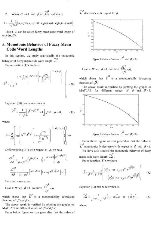
Case 2: When β >1, we have d L 0,
d
β
β
<which shows that Lβ is a monotonically decreasing
function of
β
.
The above result is verified by plotting the graphs on
MATLAB for different values of
β
andβ
>1.Figure 2. Relation between Lβ and β( 0)> .
From above figure we can generalize that the value of
L
βmonotonically decreases with respect to β and β >1.We have also studied the monotonic behavior of fuzzy
mean code word length Lαβ.
From equation (17), we have
{
}
{
}
1 ( ) (1 ( )) 1
. 1
1 1 1
2 2
( ) (1 ( ))
ni
x x D
n A i A i
L
i ni
xi xi D
A A
α α
α α
µ µ
β
α α β β
β
β β
µ µ
− + −
= ∑
−
− − = −
− + −
(32)
Equation (32) can be rewritten as
1
(1 ) (1 ) ,
1 1
2 2
Lαβ = α −β −α Lα − −β Lβ
− − (33)
{
}
1 1 1( ) (1 ( )) 1
1 1
n
n i
L xi xi D
A A
i
α
α α
µ µ
α α
−
= ∑ + − −
= −
and
{
}
1 11
( ) (1 ( )) 1 .
1 1
n
n i
L A xi A xi D
i
β
β β
µ µ
β β
−
= ∑ + − −
= −
Differentiating (33) with respect to
α
,
we have(
)
1
2 log 2
(1 ) (1 )
2 1 1
2 2
1
(1 ) .
1 1
2 2
L
L L
d L L d
β α
α α α β β
α α β
α
α α
β
α α
− ∂
= − − −
∂ − − −
+ − − −
− −
{
}
(
)
1
1 1
2 (1 ) log 2 1 2 2 (1 ) log 2 2
1 1
2 2
(1 )
. 1
1
2 2
L L L
L
d L d
β α α α α β α β β
α
α α β
α α
β
α α
−
− − − + − − −
∂ =
∂ − − −
−
+ −
− −
Here two cases arise:
Case 1: When 0< <α 1,β >1,Lα >Lβ,we get
0
L
α
β
α
∂ > ∂ ,
which shows that
L
αβ is a monotonically increasingfunction of
α
.
The above result is verified by plotting thegraphs on MATLAB for different values of
α α
( <1)andfixed value of
β
.Figure 3. Relation between Lαβ and α( 0)< .
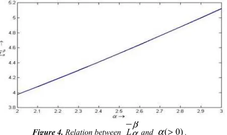
Case 2: When α >1,0< <β 1,Lα <Lβ,we have
0
L
α
β
α
∂ > ∂ ,
which shows that Lαβ is a monotonically decreasing
function of
α
.
The above result is verified by plotting thegraphs on MATLAB for different values of
α α
( >1)andfixed values of
β
.Figure 4. Relation between Lαβ and α( 0)> .
Again differentiating (33) with respect to β,we have
(
)
1
2 log 2
(1 ) (1 )
2 1 1
2 2
1
(1 ) .
1 1
2 2
L
L L
d L L d
β β
α α β
α β
β α β
β
β β
β
α α
−
∂ −
= − − −
∂ − − −
− − − −
− −
{
}
(
)
1 1 1
2 (1 ) log 2 1 2 2 (1 ) log 2
2 1 1
2 2
(1 )
. 1 1
2 2
L L L
L
d L d
β β α β
β α
β β α
α
β α β
β β
β
α β
− − − + − − − −
∂ =
∂ − − −
−
− −
− −
Here two cases arise:
Case 1: When 0< <α 1,β >1,Lα >Lβ,we get
0
Lαβ
β ∂
> ∂ ,
which shows that Lαβ is a monotonically increasing
function of
β
.Case 2: When α >1,0< <β 1,Lα <Lβ,we have
0
Lαβ
β ∂
> ∂ ,
which shows that Lαβ is a monotonically increasing
References
[1] A. De Luca and S. Termini, “A definition of non probabilistic entropy in setting of fuzzy set theory”, Inform. Contr., 20 (972), pp. 301-312.
[2] A. Renyi, “On measures of entropy and information”, Proceedings 4th Berkeley Symposium on Mathematical Statistics and Probability, 1 (1961), 547-561.
[3] B. D. Sharma and D. P. Mittal, “New non- additive measures of entropy for discrete probability distributions”, J. Math. Sci (Calcutta), 10 (1975), 28-40.
[4] B. D. Sharma and I. J. Taneja, “Three generalized additive measures of entropy”, Elec. Inform. Kybern., 13 (1977), pp. 419-433.
[5] C. E. Shannon, “A mathematical theory of communication”, Bell Syst. Tech. J., 27 (1948), pp. 379-423 & 623-659. [6] D. Bhandari, N. R. Pal and D.D. Majumder, “Fuzzy
divergence, probability measure of fuzzy events and image thresholding”, Pattern Recognition Letters, 1 (1992), 857-867.
[7] D. S. Hooda and Divya Jain, “Sub additive measures of fuzzy information”, Journal of Reliability and Statistical Studies, 02 (2009), pp. 39-52.
[8] D. S. Hooda, “On generalized measures of fuzzy entropy”, Mathematica Slovaka, 54 (2004), pp. 315-325.
[9] J. N. Kapur, “Measures of fuzzy information”, Mathematical Science Trust Society, New Delhi (1997).
[10] L. A. Zadeh, “Fuzzy sets”, Inform. Contr., 8 (1965), pp. 338-353.
[11] L. G. Kraft, “A device for quantizing grouping and coding amplitude modulated pulses”, M. S. Thesis, Electrical Engineering Department, MIT (1949).