www.nat-hazards-earth-syst-sci.net/13/3395/2013/ doi:10.5194/nhess-13-3395-2013
© Author(s) 2013. CC Attribution 3.0 License.
Natural Hazards
and Earth System
Sciences
Toward a possible next geomagnetic transition?
A. De Santis1,2, E. Qamili1, and L. Wu3,4
1Istituto Nazionale di Geofisica e Vulcanologia, Sezione Roma 2, Roma, Italy 2Università “G. D’Annunzio”, Campus Universitario, Chieti, Italy
3Northeastern University, Shenyang, China
4China University of Mining and Technology, Xuzhou, China
Correspondence to: A. De Santis ([email protected])
Received: 12 June 2013 – Published in Nat. Hazards Earth Syst. Sci. Discuss.: 27 September 2013 Revised: – – Accepted: 28 November 2013 – Published: 23 December 2013
Abstract. The geomagnetic field is subject to possible rever-sals or excursions of polarity during its temporal evolution. Considering that: (a) in the last 83 million yr the typical av-erage time between one reversal and the next (the so-called chron) is around 400 000 yr, (b) the last reversal occurred around 780 000 yr ago, (c) more excursions (rapid changes in polarity) can occur within the same chron and (d) the geo-magnetic field dipole is currently decreasing, a possible im-minent geomagnetic reversal or excursion would not be com-pletely unexpected. In that case, such a phenomenon would represent one of the very few natural hazards that are re-ally global. The South Atlantic Anomaly (SAA) is a great depression of the geomagnetic field strength at the Earth’s surface, caused by a reverse magnetic flux in the terrestrial outer core. In analogy with critical point phenomena charac-terized by some cumulative quantity, we fit the surface ex-tent of this anomaly over the last 400 yr with power law or logarithmic functions in reverse time, also decorated by log-periodic oscillations, whose final singularity (a critical point tc)reveals a great change in the near future (2034±3 yr),
when the SAA area reaches almost a hemisphere. An inter-esting aspect that has recently been found is the possible di-rect connection between the SAA and the global mean sea level (GSL). That the GSL is somehow connected with SAA is also confirmed by the similar result when an analogous critical-like fit is performed over GSL: the corresponding critical point (2033±11 yr) agrees, within the estimated er-rors, with the value found for the SAA. From this result, we point out the intriguing conjecture thattcwould be the time
of no return, after which the geomagnetic field could fall into an irreversible process of a global geomagnetic transition that could be a reversal or excursion of polarity.
1 Introduction
The magnetic field of the Earth changes in time and space, in an irregular fashion, including dramatic manifestations such as the geomagnetic reversals or excursions, when the magnetic polarities exchange in sign, so that the geomag-netic south becomes north and vice versa (e.g., Jacobs, 1994). Over the last 83 million years we count 184 reversals (Cande and Kent, 1995). From the facts that: (a) the typical average time between a reversal and another (the so-called chron) is around 400 000 yr, (b) the last reversal occurred around 780 000 yr ago, (c) more excursions (rapid changes in polar-ity) can occur within the same chron and (d) the geomagnetic field dipole is currently decreasing, a possible imminent geo-magnetic reversal or excursion would not be completely un-expected. Such a phenomenon would represent one of the very few natural hazards that are really global, because it would affect the whole globe, although the detailed conse-quences over the planet, in general, and the biosphere, in par-ticular, are not completely known. For instance, we recall a presumed link with mass extinctions (Raup, 1985; Courtillot and Besse, 1997; but see also Constable and Korte, 2006).
in the Earth’s core (Olson and Amit, 2006). Most of this decay stems from the Southern Hemisphere, as shown by Gubbins (1987), who also suggested a direct correlation be-tween the dipole decrease and the westward movements of a pair of reverse fluxes under South Africa. Other studies (e.g., Hulot et al., 2002; Constable, 2011) confirm the pres-ence, at the core mantle boundary (CMB), of two reverse flux features: in particular, one is placed inside the tangent cylinder near the North Pole and the other is a large reverse flux patch under the Southern Atlantic that has been asso-ciated with the rapid decay of the field strength. Other au-thors have concentrated their studies on understanding the mechanism of magnetic polar reversals in dynamo numerical models (e.g., Glatzmaier and Roberts, 1995). Flux patches of reversed polarity appear at low or mid latitude prior to a reversal and then migrate polewards, thus reducing the ax-ial dipole component (Wicht and Olson, 2004; Takahashi et al., 2005; Aubert et al., 2008; Wicht et al., 2009; Wicht and Christensen, 2010; Christensen, 2011). All these results are in agreement with early stages of a dipole collapse in the nu-merical dynamo model by Olson et al. (2009). In a detailed study of the Matuyama–Brunhes polarity reversal (Leonhardt and Fabian, 2007) and Laschamp excursion (Leonhardt et al., 2009) the field instability starts when reverse flux patches ap-pear in low or mid latitude regions at the CMB and then move poleward. In contrast, Aubert et al. (2008) found a mixed be-havior, with reversals and excursions initiated by reversed flux generated both outside and inside the tangent cylinder. The same authors suggested that the appearance of the South Atlantic reversed flux patch could be attributed to a reverse magnetic anticyclone supplied by a strong equatorial mag-netic upwelling.
The most recent geomagnetic dipole field is decreasing very rapidly and its temporal linear extrapolation would pre-dict a null field at around 1000 yr from now. In some parts of the Earth’s surface this zero value would be reached even earlier since this field is more complex than a pure dipolar field: for instance, in the polar regions the field would be zero in around 300 yr (De Santis, 2007). Some other papers (De Santis et al., 2004; De Santis and Qamili, 2008, 2010a) have found clear evidence for a chaotic state of the present geo-magnetic field. De Santis (2007, 2008) calculated the Shan-non information, which is a measure of the spatial order, for the field of the last 400 yr. He found that the Shannon in-formation started to decay from around 1690, and began to decrease more rapidly at around 1775 and even more rapidly after 1900, revealing that the field is increasing its overall complexity. The author also found that some parts of the globe (e.g., Antarctica) contribute more than others to this trend, in agreement with what was found by Gubbins (1987). All these aspects can be interpreted as a sign that the Earth’s magnetic field might be in the early stage of a re-versal (Hulot et al., 2002; De Santis et al., 2004; but see also Constable and Korte, 2006). Other authors, studying the fu-ture evolution of the field from numerical dynamos, use more
caution in interpreting these results (Hulot et al., 2010). Ana-lyzing the exponential growth of errors in numerical models, these authors concluded that predictions for the next reversal will not be possible for more than one century, although bet-ter predictions for the evolution of the field in the near future could be possibly made.
In the next section we will introduce some concepts related to critical point processes, i.e., dynamical systems coping with dramatic changes of state, and then we will apply these con-cepts to the temporal evolution of SAA area extension over the last 400 yr, together with the changes in the mean global sea level (GSL) as provided by Jevrejeva et al. (2008) and Church and White (2011) (but for an alternative view on GSL please see Mörner, 2004, 2010). The comparison between SAA and GSL is important because an unexpectedly close correlation between these quantities has recently been found (De Santis et al., 2012). Our joint analysis will confirm the existence of a tipping point for both time series. Finally we will present some conclusions and discussions.
2 Critical point processes and critical time
Many complex systems have “critical” thresholds (the so-called critical or tipping points) at which the system moves abruptly from one state to another, i.e., shifts toward a crit-ical transition (Scheffer, 2009); the corresponding times are also called critical times. In the literature we can find differ-ent methods for scidiffer-entific predictions of catastrophic evdiffer-ents based on the concepts of non-linear physics (e.g., Bunde et al., 2002; Dakos et al., 2012). A way to attempt to recognise these critical transitions is to detect some early warnings that may anticipate them (Scheffer et al., 2009). This strategy has been applied in ecology, medicine and global finance (May et al., 2008). Another approach is related to the critical point hypothesis for processes usually characterized by some cu-mulative critical quantity. This approach has also found ap-plications in such different fields as: climate dynamics, seis-mology, material rupture, financial crashes, etc. (Sornette, 2003). It is important to note that the critical point hypoth-esis can be used when the system is close to or moving to-ward a critical state, in analogy with a phase transition (e.g., Stanley, 1971), and the capability to predict the critical point generally improves as the latter is more approaching. With the term “critical” we denote the state of a system between order and disorder, and which is strongly influenced by ex-ternal and inex-ternal factors. Examples of systems that respond to such characteristics are some cases of liquids and mag-nets, but many others can be found in different disciplines (Sornette, 2006; Scheffer et al., 2012).
In analogy with standard critical phenomena of solid state physics, it is thought that the precursory seismicity of large events may follow power laws or alternative diverging func-tions in time. This approach has found more applicafunc-tions in the attempt to predict large earthquakes, although mostly from a retrospective point of view. In particular, Bufe and Varnes (1993) and Bowman et al. (1998) suggested that the timetc of the largest main shock of a seismic sequence is
the critical time of the seismic sequence, i.e., the time when the system drastically changes its dynamical regime. Since the seismological phenomena are mainly earthquakes, which
are large ruptures or failures of a part of the crust, this ap-proach has also been called the “time-to-failure” apap-proach. In a broad sense, also in other occasions and fields when a general system shifts to a critical transition, the latter event could be considered as a failure of the system to maintain its previous typical state; thus the term failure must be taken in this general meaning, not implying necessarily that there is a physical failure or rupture in the system under study. Then, a measurey(t )of the seismic release (e.g., the seismic defor-mation) at any preceding timetreasonably close to the time tccan be described by a power law relation of the form:
y(t )=k(tc−t )−n (1)
where k >0 and 1> n >0 are appropriate parameters. Equation (1) is characterized to have a singularity att=tc
becausey(tc)= ∞. In practice, in seismology it is preferred
to integrate Eq. (1) in time to use a cumulative functions(t ) ofy(t ), in order to have a finite value fors(tc), its time
deriva-tive being singular, i.e., the slope of the functions(t )attcis
vertical. In this way, we have: s(t )=
Z
y(t )dt=a− k m(tc−t )
m=a+b(t
c−t )m (2)
where a> 0 is the constant of integration; b= −k/m <0, andm=1−n > 0 are constant parameters that are found by means of a nonlinear least regression on the available data; m, normally 0.2 <m< 0.6 (Mignan, 2011), is a critical expo-nent that represents the degree of accelerating energy release (De Santis et al., 2010). It is clear thata is the value of the measure related to the cumulative seismic release at the crit-ical time, i.e.,a=s(tc). In addition to the accelerating strain
release in Eqs. (1) or (2), Sornette and Sammis (1995) pro-posed an extension of this method, finding a better fit to the time of occurrence of large seismic events by fitting a func-tion that included a log-periodic fluctuafunc-tion:
s(t )=a+b(tc−t )m· {1+d·cos[2πfln(tc−t )+ϕ]} (3)
whered is the magnitude of the fluctuations around the ac-celeration growth,f is the frequency of the fluctuations,ϕis the phase shift, andtcis the critical time. Note that ford=0
we have the simple power law as in Eq. (2). The equations from Eqs. (1) to (3) have also been applied in analyzing fi-nancial crises (Sornette, 2003).
An alternative form of diverging functions in time is that of considering just a logarithmic function in (reversed) time (e.g., Vandewalle et al., 1998):
s(t )=A+Bln(tc−t ) (4)
whereA> 0 and B< 0 (andtc) are parameters to be found
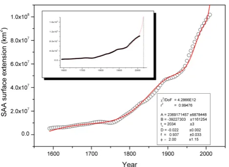
Fig. 1. Extension of the SAA over the last 400 yr and the best non-linear fit of the function indicated in the text as Eq. (5). The “critical time”tcwould be 2034±3 yr, where the curve will have a singular-ity, i.e., where the curve is tangent to the vertical dashed line drawn at the critical time in the smaller picture. Our interpretation is that this time will represent the time of no return for a great change in the geomagnetic field, possibly going toward a reversal or excursion. In the inset table, DoF are the degrees of freedom andris the correla-tion coefficient of the nonlinear fit; for the other fitting parameters see the text.
calculations the time is in years, the value ofAis a good ap-proximation of the actual value that the quantity under study will take close to its critical time (i.e., just one year before). Equation (4) is the time integral of the limiting case of Eq. (1) withn=1, andAis the constant term of integration. The cor-responding log-periodic form can be written as (e.g., Vande-walle et al., 1998):
s(t )=A+Bln(tc−t )·{1+D·cos[2πfln(tc−t )+ϕ]}. (5)
Note that forD=0 we have simple logarithmic divergence as in Eq. (4).
It is clear that the “integral” Eqs. (2)–(5) are more appro-priate than Eq. (1) for SAA and GSL, because they are all cumulative processes as the seismic deformation for which some of those equations had been introduced.
The quality of the acceleration toward the critical point can be evaluated by theC factor (Bowman et al., 1998), which measures the ratio between the root mean squares (rms) of the diverging function (rmsdf)and the rms of the best fit line
(rmsline):
C= rmsdf rmsline
=
s
1−rdf2
1−rline2 (6)
wherer is the correlation coefficient of the corresponding fit. The lower than 1 theC factor is, the greater (and more significant) the acceleration toward the critical point is.
In the next section we will analyze the SAA at the Earth’s surface, because the geomagnetic field is known there and
Fig. 2. Global sea level (GSL) rise and its best log-periodic fit with Eq. (5). The critical time (2033±11 yr indicated by the vertical dashed line in the smaller picture) within the given error is the same as that estimated for the SAA. In the inset table, DoF are the degrees of freedom andris the correlation coefficient of the nonlinear fit; for the other fitting parameters see the text.
any global model is more reliable at the Earth’s surface than at that extrapolated at the CMB, where the main sources of the geomagnetic field are placed (e.g., Merrill and McEl-hinny, 1983): the higher harmonics, which are typically mea-sured at the surface with a low signal-to-noise ratio, are greatly amplified together with their errors, when extrapo-lated downward to the CMB, contaminating any final rep-resentation of the field at that depth (Lowes, 1974). In the Appendix we show that the critical timetcfor the SAA is as
important at the Earth’s surface as at the CMB.
3 Application to SAA and GSL data and interpretation: a great planetary change?
We applied all possible functions given by Eqs. (1)–(5) over the SAA and GSL data. In our study the log-periodic ap-proach Eq. (5) has shown the best fit over the available data with respect to the other possible functions in terms of the lowestχ2and the highest correlation coefficientr. Figures 1 and 2 show the corresponding results for SAA and GSL, re-spectively. A lowCfactor (0.18 and 0.48 for SAA and GSL, respectively) confirms a significant acceleration toward the critical point. When we compare the couples of the same fit-ting parameters with each other, the agreement is astonishing for most of them: in particular, the critical timetc is
analyses we did not consider any error in the SAA area esti-mates. Defining an accurate error budget for the area of the SAA is not possible.
Not only has one to find what the accuracy of the Gauss coefficients is, but one also has to estimate what the contri-butions of the unknown small scales of the magnetic field are. One also has to estimate what effect the regularization process (if present) applied for deriving magnetic field mod-els from geomagnetic data has on the SAA area. Neverthe-less we expect that the greatest contribution will come from the Gauss coefficient errors, so we try to take them into ac-count in a simple way. Likely, errors in the Gauss coeffi-cients change with time, say from 10 % at the beginning of the considered time interval and 1 % in more recent times, so we cannot be too wrong in supposing an average crude error budget of 5 % to propagate with the same percentage to the SAA area values. When these errors are considered in a weighted log-periodic fit the results (not shown here) are not significantly different from those above (in particular, we find a critical time of 2042). Therefore, in all cases a criti-cal process is still compatible with model data. This means that the overall trend that underlies both quantities (SAA and GSL) is something real and not an artefact. This confirms the choice of De Santis et al. (2012) to make the compari-son of SAA and GSL (in terms of Spearman rank correlation and relative entropy) without removing any trend (although, when removing a trend and normalizing both time series to unitary standard deviation, correlation still remains signifi-cant, with the Pearson correlation coefficientr=0.62 and P <0.0001; this correlation increases much more when we consider more recent data after 1800, reachingr=0.94 and P <0.0001). The low values ofχ2/ DoF (degrees of free-dom) and the high values of the correlation coefficientr(for both quantitiesr> 0.98), with respect to the corresponding fit, indicate that the acceleration of both SAA and GSL is un-likely to be a mere coincidence, and that they are, rather, in-dications of some physical underlying critical point process. Also, theDandf parameters are very similar in both SAA and GSL, indicating that the fluctuations affect the acceler-ation in almost the same way in both physical quantities. In addition, it is interesting to note that the critical time of the SAA will be almost the time at which the SAA area, i.e., the parameterA, will cover a hemisphere: because of the valid-ity of Eqs. (A2) and (A3), this is limited not only to the field at the Earth’s surface, but would also be at the CMB, where A0 of Eq. (A4) will cover more than half of the core sur-face. Since the SAA is usually considered the manifestation at the Earth’s surface of a reversal magnetic flux produced at the CMB (e.g., Hulot et al., 2002), the epoch when the SAA may reach the area corresponding to the surface of half the planet is a critical moment for the present geomagnetic field. This time is not the time of the eventual geomagnetic rever-sal, but we interpret it as the time of the point of no return, after which the geomagnetic field could fall in the process of a global geomagnetic transition, which could be a
rever-sal or excursion of polarities. How long after the critical time tc this transition will occur cannot be fully established,
be-cause what we predict is a time when the dynamical system reaches its critical state, after which any successive time is a potential candidate for the actual start of the reversal or excursion. Why GSL also shows the same overall trend with similar parameters is a question that deserves further scrutiny and is left to future work. What we can speculate now is that when GSL reaches its critical point it will correspond to a significant coverage of many present coasts, implying a big change in the land–ocean system. In addition, the similarities found in both SAA and GLS confirm that the two quantities are really closely related, and, if the interpretation of an im-minent geomagnetic field reversal is correct, this would once more support the internal hypothesis indicated among other possibilities in De Santis et al. (2012).
4 Conclusions
In this work we analyze both SAA and GSL overall trends in the last few centuries, finding an astonishing similarity, further confirming previous results (De Santis et al., 2012). These similar trends can be explained by the theory of the critical point processes for which each dynamical system is close to or is going toward a critical point, when the system will undergo a dramatic change in its macroscopic proper-ties. This interpretation comes from the analysis of the SAA behavior, for which the critical timetcwould correspond to
practically the time at which the SAA area will exceed the extent of a hemisphere. Since SAA is a superficial manifes-tation of a reverse magnetic flux at the CMB, this time will be the time of no return after which the geomagnetic field will go to a significant transition reverse in polarity, such as a geomagnetic excursion or a complete geomagnetic reversal.
A similar dramatic change would have to occur in the oceans, although no clear information can be obtained from the present work. Regarding this, only some questions can be asked: would the entire Earth or most of it be flooded? This seems not to be the case, because from a simple calcula-tion (Woo, 2011), the predicted sea level rise of around 0.5 m higher than the present value (at timetc−1) will cause about
3 km of present coasts to be covered by water. Nevertheless, if this is the case, the consequences will be very dramatic as well (let us think of the many cities and mega-cities that are close to the coasts). Or would the GSL suddenly collapse? Or would the GSL’s abrupt increase imply an enormous change in the land–ocean system? Or what else? In this sense, if the model we propose for both SAA and GSL is correct, what is in preparation will be a really global change, and many more parts of the planet could be involved, humankind included.
fit, although this could simply be due to some edge effects in the IGRF-11 model construction that we used for the most recent years. Second, because of its intrinsic chaotic char-acteristics (De Santis et al., 2004), the time of predictability of the geomagnetic field is comparable with the remaining time to the predictedtc(e.g., De Santis et al., 2004; Hulot et
al., 2010). Thus, the prediction of the critical time should be updated again as soon as more SAA and GSL data become available, since any prediction based on a log-periodic func-tion such as Eq. (5) is not stable when we are far from the critical time, but improves its quality of prediction as soon as we are closer totc(e.g., Brée and Joseph, 2013). The study
of the diverging function parameters at successive predic-tions/times together with the use of theC factor will also allow one to investigate any deviation of the real behavior from the prediction, and possibly to detect a change from the present “catastrophic” trend: any departure from the behavior predicted so far would be seen in terms of significant increase of bothtc and theC factor. Third, both SAA and GSL can
also be well fitted by some higher degree polynomial: for ex-ample, a quintic polynomial (containing the same number of unknown coefficients of our log-periodic function) provides, in terms ofr2andχ2/ DoF, a fitting quality similar to that obtained by the log-periodic function, although, of course, the found polynomial behaves unrealistically outside the data range, thereby excluding its use for forecasting purposes.
Now one might ask why we are able to predict the point of no return from just a few hundred years of a phenomenon that usually lasts several thousand years (Jacobs, 1994; but see also Nowaczyk et al., 2012, where the Laschamp excur-sion seems to change the geomagnetic polarity in a few hun-dred years), i.e., with some analysis based on data taken over a temporal window much shorter than the typical timescales of the reversal or excursion process. A simple answer is that we are analyzing a sufficient (although short) time before the eventual critical transition: we believe that the recent accel-eration of both SAA and GSL is nothing casual, but probably uncovers important physical information regarding the future of our planet in the near future, such as a possible precursor to the eventual close critical transition of the geomagnetic field.
Appendix A
This appendix has the aim of showing that the results ob-tained by means of analyses made on the SAA at the Earth’s surface are equivalent to those made at the CMB, where the main sources of the geomagnetic field are placed, but where any extrapolation is difficult or even impossible.
However complicated the geomagnetic field may be at the SAA within the 32 000 nT isoline, we can define a frus-tum of quasi-conethat is confined by the lower surface S(rCMB)at the CMB, i.e., atr=rCMB=3485 km and the
upper surfaceS(r0)of the SAA at the Earth’s surface, i.e., at
Fig. A1. The magnetic flux crossing both the core mantle bound-ary (CMB) and South Atlantic Anomaly (SAA) is conserved. Thus analyses on the SAA at the Earth surface are equivalent to those made at the CMB.
r=r0=6371 km (Fig. A1); the lateral surface is here called Sl. The lower surfaceS(rCMB)at the CMB is representative
of some typical isoline enclosing the reverse magnetic flux (we will come back to this in the final part of the Appendix). The divergence-free condition of the geomagnetic field imposes a null flux through the surfaces bounding the vol-ume:
8[S(rCMB)] −8[S(r0)] −8[Sl] =0 (A1)
where8[Si]is the magnetic flux across the surfaceSi(where
SiisS(r0)orS(rCMB)orSl)that can be expressed as follows:
8[Si] =
Z
Bi·ndSi=BicosδSi
whereBicosδis the mean component of the field
perpendic-ular to the surfaceSi (δis the angle between the vector field
B and the vectornnormal toSi). For the geometry of the
quasi-conical volume,Bicosδwill beZfor the upper SAA
and the lower surface at the CMB, while it will be a compo-nent in the horizontal plane for the lateral surfaceSl. We can
safely neglect the flux across the lateral surfaceSlof; thus
Eq. (A1) becomes:
Z(rCMB)S(rCMB)=Z(r0)S(r0) (A2)
and S(rCMB)=
Z(r0) Z(rCMB)
S(r0)=γ S(r0),
where theγ ratio
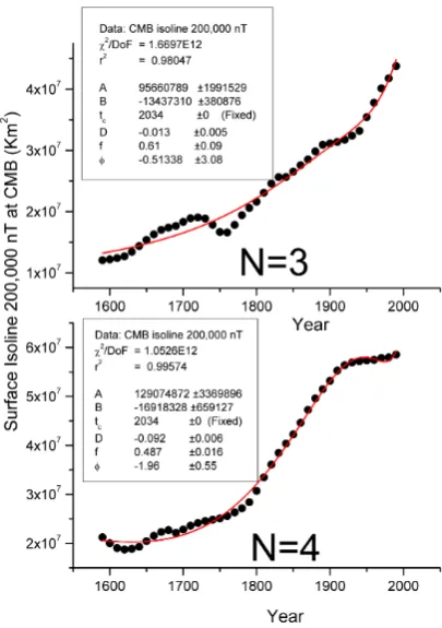
Fig. A2. Surface enclosed by the isoline 200 000 nT at the CMB for an expansion of GUFM1 up to the spherical harmonic degree
N=3 andN=4. Both trends are almost monotonic and diverging in time. A log-periodic function with critical (a priori fixed) time of 2034 yr is a reasonable fit for both cases.
can be taken as constant in time. This means that an equation of the same form as Eq. (4) (but this would also be valid for Eq. 5) can also be written fors0(t )ofS(rCMB):
s0(t )=A0+B0ln(tc−t ), (A4)
withA0=γ AandB0=γ B. Thus, the results we find at the Earth’s surface are also representative of the deep dynamics of the geomagnetic field; in particular, the critical timetc
es-timated at the Earth’s surface will also be the same for the CMB.
Unfortunately it is difficult to verify the constancy ofγ with any global model (such as GUFM1) that is based on ob-servational data taken at the Earth’s surface. This difficulty is twofold: (i) the areaS(rCMB)is impossible to determine, and
(ii) it is difficult or even impossible to estimateZ(rCMB)
be-cause of the eventual explosion of errors when continuing the vertical component from the Earth’s surface to the CMB, be-cause of their multiplication by a factor [r0/ rCMB]n+2(nis
here the spherical harmonic degree of the geomagnetic field expansion).
To reasonably circumvent most of the problems, we can simply look at an isoline at the CMB that could act as the 32 000 nT at the Earth’s surface. By applying a simple dipolar
downward continuation of the 32 000 nT isoline to CMB (just multiplying by [r0/rCMB]3) we obtain about 200 000 nT.
Therefore, looking at the surface enclosed by the latter iso-line at the CMB for an expansion of the GUFM1 model up to N=3 andN=4 (Fig. A2), we notice an almost monotonic trend for both cases where a log-periodic behavior pointing to a critical (a priori fixed) time of 2034 is something really possible (Cfactor is always much less than 1 for both cases: 0.52 and 0.23 forN=3 and 4, respectively). By the way, the area of the enclosed surfaces 1 yr before the critical time for N=3 andN=4 are 64 % and 84 %, respectively, so in both cases the surface of this isoline at the critical time will cover more than half of the entire core surface. We limit our anal-ysis made at the CMB toN=4, because for larger values of N, the expected downward continuation errors would be too large to reliably detect the 200 000 nT (or any other) isoline.
Acknowledgements. Part of this work has been realised in the
frame of the SAGA-4-EPR project co-funded by the Italian Foreign Office, the Istituto Nazionale di Geofisica e Vulcanologia (Italy) and Northeastern University of Shenyang (China). We thank G. Hulot, G. Balasis and P. Lurcock, whose constructive comments helped us to improve a preliminary version of this manuscript. We also thank two anonymous referees for their comments and suggestions.
Edited by: R. Lasaponara
Reviewed by: two anonymous referees
References
Amit, H., Leonhardt, R., and Wicht, J.: Polarity reversals from paleomagnetic observations and numerical dynamo simulations, Space Sci. Rev., 155, 293–335, 2010.
Aubert, J., Aurnou, J., and J. Wicht, J.: The magnetic structure of convection-driven numerical dynamos, Geophys. J. Int., 172, 945–956, 2008.
Bowman, D. D., Ouillon, G., Sammis, C. G., Sornette, A., and Sor-nette, D.: An observational test of the critical earthquake concept, J. Geophys. Res., 103, 24359–24372, 1998.
Brée, D. S. and Joseph, N. L.: Testing for financial crashes using the log periodic power law model, International Review Financial Analysis, 30, 287–297, 2013.
Bufe, C. G. and Varnes, D. J.: Predictive modelling of the seismic cycle of the Greater San Francisco Bay region, J. Geophys. Res., 98, 9871–9883, 1993.
Bunde, A., Kropp, J., and Schellnhuber, H. J.: The Science of Dis-asters. Climate disruptions, heart attacks, and market crashes, Springer Berlin, 2002.
Cande, S. C. and Ken, D. V.: Revised calibration of the geomag-netic polarity timescale for the late Cretaceous and Cenozoic, J. Geophys. Res., 100, 6093–6095, 1995.
Christensen, U. R.: Geodynamo models: Tools for understanding properties of the Earth’s magnetic field, Phys. Earth Planet. Int., 187, 157–169, 2011.
Constable, C. G.: Modelling the geomagnetic field from syntheses of paleomagnetic data, Phys. Earth Planet. Int., 187, 109–117, 2011.
Constable, C. G. and Korte, M.: Is Earth’s magnetic field reversing?, Earth Planet. Sci. Lett., 246, 1–16, 2006.
Courtillot V. and Besse J.: Magnetic Field Reversals, Polar Wander, and Core-Mantle Coupling, Science, 237, 1140–1145, 1987. Dakos, V., Carpenter, S. R., Brock, W. A., Ellison, A. M., Guttal, V.,
Ives, A. R., Kéfi, S., Livina, V., Seekell, D. A., van Nes, E. H., and Scheffer, M.: Methods for detecting early warnings of critical transitions in time series illustrated using simulated ecological data, PLoS One, 7, e41010, doi:10.1371/journal.pone.0041010, 2012.
De Santis, A.: How persistent is the present trend of the geomag-netic field to decay and, possibly, to reverse?, Phys. Earth Planet. Int., 162, 217–226, 2007.
De Santis, A.: Erratum to “How persistent is the present trend of the geomagnetic field to decay and, possibly, to reverse?”, Phys. Earth Plan. Int., 170, p. 149, 2008.
De Santis, A. and Qamili, E.: Are we going towards a global planetary magnetic change? 1st WSEAS International Confer-ence on Environmental and Geological SciConfer-ence and Engineering (EG’08), 149–152, 2008.
De Santis, A. and Qamili, E.: Shannon information of the geomag-netic field of the past 7000 years, Nonlin. Proc. Geophys., 17, 77–84, 2010a.
De Santis, A. and Qamili, E.: Equivalent monopole source of the ge-omagnetic South Atlantic Anomaly, Pure Appl. Geophys., 167, 339–347, 2010b.
De Santis, A., Tozzi, R., and Gaya-Piqué, L.R.: Information content and K-Entropy of the present geomagnetic field, Earth Planet. Sci. Lett., 218, 269–275, 2004.
De Santis, A., Cianchini, G., Qamili, E., and Frepoli, A.: The 2009 L’Aquila (Central Italy) seismic sequence as a chaotic process, Tectonophysics, 496, 44–52, 2010.
De Santis, A., Qamili, E., Spada, G., and Gasperini, P.: Geomag-netic South Atlantic Anomaly and global sea level rise: a direct connection?, J. Atmos. Sol. Terr. Phys., 74, 129–135, 2012. Finlay, C. C.: Historical variation of the geomagnetic axial dipole,
Phys. Earth Planet. Int., 170, 1–14, 2008.
Finlay, C. C., Maus, S., Beggan, C. D., Hamoudi, M., Lowes, F. J., Olsen, N., and Thebault, E.: Evaluation of candidate geomag-netic field models for IGRF-11, Earth Planets Space, 62, 787– 804, 2010.
Glatzmaier, G. A. and Roberts, P. H.: A three-dimensional self-consistent computer simulation of a geomagnetic field reversal, Nature, 377, 203–209, 1995.
Gross, S. and Rundle, J.: A systematic test of time-to-failure analy-sis, Geophys. J. Int., 133, 57–64, 1998.
Gubbins, D.: Mechanism for geomagnetic polarity reversals, Na-ture, 326, 167–169, 1987.
Gubbins, D., Jones, A. L., and Finlay, C. C.: Fall in Earth’s Mag-netic Field is erratic, Science, 312, 900–902, 2006.
Hulot, G., Eymin, C., Langlais, B., Mandea, M., and Olsen, N.: Small-scale structure of the geodynamo inferred from Øersted and Magsat satellite data, Nature, 416, 620–623, 2002.
Hulot, G., Lhuillier, F., and Aubert, J.: Earth’s dynamo limit of predictability, Geophys. Res. Lett., 37, L06305, doi:10.1029/2009GL041869, 2010.
Jackson, A., Jonkers, A. R. T., and Walker, M. R.: Four centuries of geomagnetic secular variation from historical records, Philos. Trans. R. Soc. Lond. A, 358, 957–990, 2000.
Jacobs, J. A.: Reversals of the Earth’s magnetic field, 2nd Edition, Cambridge University Press, Cambridge, UK, 346 pp., 1994. Jevrejeva, S., Moore, J. C., Grinsted, A., and Woodworth, P. L.:
Re-cent global sea level acceleration started over 200 years ago?, Geophys. Res. Lett., 35, L08715, doi:10.1029/2008GL033611, 2008.
Leonhardt, R. and Fabian, K.: Paleomagnetic reconstruc-tion of the global geomagnetic field evolureconstruc-tion during the Matuyama/Brunhes transition: iterative Bayesian inversion and independent verification, Earth Planet. Sci. Lett., 253, 172–195, 2007.
Leonhardt, R., Fabian, K. Winklhofer, M. Ferk, A. Kissel, C., and Laj, C.: Geomagnetic field evolution during the Laschamp excur-sion, Earth Planet. Sci. Lett., 278, 87–95, 2009.
Lowes, F. J.: Spatial power spectrum of the main geomagnetic field, and extrapolation to the core, Geoph. J. R. Astr. Soc., 36, 717– 730, 1974.
Malin, S. R. C.: Sesquicentenary of Gauss’s first measurement of the absolute value of magnetic intensity, Philos. Trans. R. Soc. Lond. A, 306, 5–8, 1982.
May, R. M., Levin, S. A., and Sugihara, G.: Ecology for bankers, Nature, 451, 893–895, 2008.
Merrill, R. T. and McElhinny, M. W.: The Earth’s Magnetic Field (Its History, Origin and Planetary Perspective), Academic Press, San Diego, 1983.
Mignan, A.: Retrospective on the Accelerating Seismic Release (ASR) hypothesis: controversy and new horizons, Tectono-physics, 505, 1–16, 2011.
Mörner, N.-A.: Estimating future sea level changes from past records, Global Planet. Change, 40, 49–54, 2004.
Mörner, N.-A.: Some problems in reconstruction of mean sea and its changes with time, Quatern. Int., 221, 3–8, 2010.
Nowaczyk, N. R., Arz, H. W., Frank, H. W., Kind, J., and Plessen, B.: Dynamics of the Laschamp geomagnetic excursion from Black Sea sediments, Earth Planet. Sci. Lett., 351, 54–69, 2012. Olson, P. and Amit, H.: Changes in earth’s dipole,
Naturwis-senschaften, 93, 519–542, 2006.
Olson, P., Driscoll, P., and Amit, H.: Dipole collapse and reversal precursors in a numerical dynamo, Phys. Earth Planet. Int., 173, 121–140, 2009.
Raup D. M.: Magnetic Reversals and Mass extinctions, Nature, 314, 341–343, 1985.
Scheffer, M.: Critical Transitions in Nature and Society. Princeton Univ. Press, 2009.
Scheffer, M., Bascompte, J., Brock, W., Brokvin, V., Carpenter, S. R., Dakos, V., Held, H., van Nes, E. H., Rietkerk, M., and Sug-ihara, G.: Early-warning signals for critical transitions, Nature, 461, 53–59, 2009.
Scheffer, M., Carpenter, S. R., Lenton, T. M., Bascompte, J., Brock, W., Dakos, V., van de Koppel, J., van de Leemput, I. A., Levin, S. A., van Nes, E. H., Pascual, M., and Vandermeer, J., Anticipating critical transitions, Science, 338, 344–348, 2012.
Sornette, D.: Why stock markets crash. Critical events in complex financial systems, Princeton Univ. Press, Oxford, 2003. Sornette, D.: Critical Phenomena in Natural Sciences, Second Ed.
Sornette, D. and Sammis, C.: Complex critical exponents from renormalization group theory of earthquakes: implications for earthquake predictions, J. Phys. I France, 5, 607–619, 1995. Stanley, H. E.: Phase transition and critical phenomena, Clarendon
Press, New York, 1971.
Takahashi, F., Matsushima, M., and Honkura, Y.: Simulations of a quasi-Taylor state geomagnetic field including polarity reversals on the Earth simulator, Science, 309, 459–461, 2005.
Vandewalle, N., Ausolos, M., Boveraus, P., and Minguet, A.: How the financial crash of October 1997 could have been predicted, Eur. Phys. J. B., 4, 139–141, 1998.
Wicht, J. and Christensen, U. R.: Torsional oscillations in dynamo simulations, Geophys. J. Int., 181, 1367–1380, 2010.
Wicht, J. and Olson P.: A detailed study of the polarity reversal mechanism in a numerical dynamo model, Geochem. Geophys. Geosyst., 5, Q03H10, doi:10.1029/2003GC000602, 2004. Wicht, J., Stellmach, S., and Harder, H.: Numerical models of the
geodynamo: from fundamental Cartesian models to 3-D simula-tions of field reversals, edited by: Glassmeier, K. H., Soffel, H., and Negendank, J. F. W., Geomagnetic field variations. Springer, Berlin, 107–158, 2009.