Simulating lightning into the RAMS model: implementation and

(1)

Nat. Hazards Earth Syst. Sci., 14, 2933–2950, 2014 www.nat-hazards-earth-syst-sci.net/14/2933/2014/ doi:10.5194/nhess-14-2933-2014

Simulating lightning into the RAMS model: implementation and

preliminary results

S. Federico, E. Avolio, M. Petracca, G. Panegrossi, P. Sanò, D. Casella, and S. Dietrich ISAC-CNR, UOS of Rome, via del Fosso del Cavaliere 100, 00133 Rome, Italy

Correspondence to: S. Federico ([email protected])

Received: 14 March 2014 – Published in Nat. Hazards Earth Syst. Sci. Discuss.: 12 May 2014 Revised: 4 September 2014 – Accepted: 2 October 2014 – Published: 7 November 2014

Abstract. This paper shows the results of a tailored version of a previously published methodology, designed to simu-late lightning activity, implemented into the Regional Atmo-spheric Modeling System (RAMS).

The method gives the flash density at the resolution of the RAMS grid scale allowing for a detailed analysis of the evo-lution of simulated lightning activity.

The system is applied in detail to two case studies occurred over the Lazio Region, in Central Italy. Simulations are com-pared with the lightning activity detected by the LINET net-work. The cases refer to two thunderstorms of different inten-sity which occurred, respectively, on 20 October 2011 and on 15 October 2012.

The number of flashes simulated (observed) over Lazio is 19 435 (16 231) for the first case and 7012 (4820) for the sec-ond case, and the model correctly reproduces the larger num-ber of flashes that characterized the 20 Octonum-ber 2011 event compared to the 15 October 2012 event.

There are, however, errors in timing and positioning of the convection, whose magnitude depends on the case study, which mirrors in timing and positioning errors of the light-ning distribution. For the 20 October 2011 case study, spatial errors are of the order of a few tens of kilometres and the timing of the event is correctly simulated. For the 15 Octo-ber 2012 case study, the spatial error in the positioning of the convection is of the order of 100 km and the event has a longer duration in the simulation than in the reality.

To assess objectively the performance of the methodology, standard scores are presented for four additional case studies. Scores show the ability of the methodology to simulate the daily lightning activity for different spatial scales and for two different minimum thresholds of flash number density. The

performance decreases at finer spatial scales and for higher thresholds.

The comparison of simulated and observed lighting activ-ity is an immediate and powerful tool to assess the model ability to reproduce the intensity and the evolution of the con-vection. This shows the importance of using computationally efficient lightning schemes, such as the one described in this paper, in forecast models.

1 Introduction

The lightning threat in convective thunderstorms is a signif-icant concern for public safety (Curran et al., 2000; Porcù and Carrassi, 2009) and for activities that are sensitive to this threat, such as aviation and management of electric infras-tructures.

Lightning is a characteristic of severe weather and often accompanies heavy precipitation and large hail. The rela-tionship between lightning and heavy precipitation has been studied extensively in several parts of the world (Tapia et al., 1998; Land and Rutledge, 2002; Latham et al., 2003; Soula et al., 1998; Zhou et al., 2002).

(2)

2934 S. Federico et al.: Simulating lightning into the RAMS model: implementation and preliminary results In the Mediterranean region, the relationship between

lightning and precipitation has also been studied, based on satellite (Tropical Rainfall Measuring Mission (TRMM) Lightning Image Sensor (LIS); Cecil et al., 2005; Goodman et al., 2007), and ground-based lightning location systems (Altaratz et al., 2003; Defer et al., 2005; Price and Feder-messer, 2006; Katsanos et al., 2007a, b). The FLASH project (Price et al., 2011) aimed at improving the understanding and forecasting ability of flash floods in the Mediterranean region using lightning data. It was found that real-time lightning observations on a regional basis are very useful in detect-ing, monitoring and tracking intense thunderstorm activity on large spatial scales.

These studies confirm that the lightning is related to deep convection and heavy rains. However, as pointed out by Pe-tersen et al. (2005), while the relationship between rainfall and lightning is highly regime dependent and there is a large variability of the water volume/flash found in different areas of the world, the relationship between total lightning activ-ity and ice mass is more robust. In their study they found that, on a global scale, the relationship between column in-tegrated precipitation ice mass and lightning flash density is invariant between land, ocean and coastal regimes (in con-trast to rainfall), suggesting that the physical assumptions of precipitation-based charging and mixed-phase precipitation development are robust.

Deierling and Petersen (2008) and Deierling et al. (2008) used a Doppler and dual-polarimetric radar as a source of information of ice distribution and updraft in clouds, and lightning data collected in northern Alabama and Col-orado/Kansas during two field campaigns. They showed that the updraft volume in the charging zone was highly corre-lated with total lightning activity, finding that these relation-ships are relatively invariant between different climate con-ditions.

It should also be mentioned that the lightning activity has an influence on atmospheric chemistry because of its ability to create nitrogen oxides (e.g. Grewe, 2009).

All those subjects foster the interest in observing and fore-casting lightning, as confirmed by the planned launch of a Geostationary Lightning Mapper aboard GOES-R satellites and of the Lightning Imager on METEOSAT Third Gener-ation (MTG), and the increasing interest for ground-based lightning detection networks. Moreover, there has been an increasing interest in investigating in more detail the mecha-nisms of the electrification processes, in order to find quanti-tative relationships between lightning flashes and cloud prop-erties directly connected with them, such as precipitating and non-precipitating ice mass content, and cloud updrafts. In or-der to do that, cloud electrification models are used.

Nowadays, the methods to simulate lightning in thunder-storm may be classified in two main groups. The first con-tains advanced one-dimensional (Solomon and Baker, 1996; Solomon et al., 2005; Formenton et al., 2013) or three-dimensional (Mansell et al., 2002, 2005; MacGorman et

al., 2001) cloud models equipped with sophisticated elec-trification schemes. These schemes make use of the results of laboratory experiments, which have revealed the trans-fer of charge during hydrometeor collisions (Saunders, 2008, reviews the mechanisms of charge separation in thunder-storms). In these methods the electric field and the dielectric breakdown are explicitly simulated.

These schemes were also parametrized in cloud-resolving and mesoscale models (Mansell et al., 2005; Barthe et al., 2005, 2010). Recently, Lynn et al. (2012) implemented a dynamically based algorithm into the WRF model to pro-duce forecast maps for positive and negative cloud-to-ground and intracloud lightning. Their methodology uses the dy-namic and microphysics fields from WRF to calculate the electrical potential energy for positive and negative cloud-to-ground and intracloud lightning, adding prognostic equa-tions for three variables in the WRF model. The number of cloud-to-ground (positive and negative) and intracloud light-ning is computed from these potentials, whenever the poten-tial energy is larger than a threshold energy, whose value de-pends on the type of lightning (positive and negative cloud-to-ground and intracloud). Scores for seven case studies in-dicate that the methodology is able to predict the occurrence of the positive and negative cloud-to-ground and intracloud events.

The second group contains simple schemes that corre-late the hydrometeors or other parameters computed by cloud-resolving models (nowadays with horizontal resolu-tion ≤3 km) with the number of observed flashes, giving the flash rate (Price and Rind, 1992; McCaul et al., 2009; Yoshida et al., 2009; Yair et al., 2010; Wong et al., 2013). Wong et al. (2013), revised the Price and Rind parametriza-tions by applying the methodology in cloud-resolving mod-els. They showed the need for a validation and tuning of the parametrizations when applying the method to cloud-resolving models.

These schemes have the advantage of being simple and computationally efficient, giving a tool for implementing the lightning forecast operationally. Moreover, several of the above-mentioned papers show the superiority of these schemes compared to a former generation of methods that have been based on the correlation between thunderstorm occurrence and thermodynamic indices (e.g. Bright et al., 2004).

(3)

S. Federico et al.: Simulating lightning into the RAMS model: implementation and preliminary results 2935

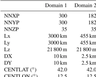
Table 1. RAMS grid setting. NNXP, NNYP and NNYZ are the

number of grid points in the west–east, north–south, and vertical di-rections. Lx (km), Ly (km), Lz (m) are the domain extension in the west–east, north–south, and vertical directions. DX (km) and DY (km) are the horizontal grid resolutions in the west–east and north– south directions. CENTLON and CENTLAT are the geographical coordinates of the grid centres.

Domain 1 Domain 2

NNXP 300 182

NNYP 300 182

NNZP 35 35

Lx 3000 km 455 km

Ly 3000 km 455 km

Lz 21 800 m 21 800 m

DX 10 km 2.5 km

DY 10 km 2.5 km

CENTLAT (◦) 42.0 42.0

CENTLON (◦) 12.5 12.5

convective rainfall, while it is well correlated with the simu-lated concentrations of solid hydrometeors.

This paper shows the implementation of a methodology to simulate lightning activity in the RAMS model and shows the results of its application to six case studies in Central Italy. Two of these cases are analysed in detail, while statis-tical scores are presented for all cases. The method used in this study belongs to the second group of methods to sim-ulate lightning in cloud-resolving models described above, because it is rather simple and computationally efficient.

The approach is a tailored form of the method of Dahl et al. (2011a, b), hereafter DHS1 and DHS2. In particular, DHS1 shows the theoretical underpinnings of the scheme im-plemented and the reader should refer to this work for a de-tailed discussion of the physical foundation of the method-ology, while DHS2 discusses its practical implementation in the COSMO (Consortium for Small Scale Modeling) model. The methodology presented in this paper differs from DHS1 and DHS2 because it is designed to account for the differences of RAMS with respect to the COSMO model and to focus on the charge separation processes occurring in the charging zone, and it also uses a different method to spatially distribute the simulated lightning associated with the convec-tive cells.

The paper is organized as follows: in Sect. 2 the RAMS model is introduced, as well as the details of the methodology used in this work, and the lightning detection network used for comparison with the model results. Section 3 shows in detail the results of two case studies which occurred over the Lazio Region, in central Italy, as well as the scores for these two cases. To make the results statistically more robust, and to define better the limits of applicability of the methodology presented in this paper, scores of four additional cases are

37 Figures

1 2

3 4

Figure 1: Domains used in this paper (D1, D2) and the Lazio Region (L) in the 5

second domain. 6

7

Figure 1. Domains used in this paper (D1, D2) and the Lazio

Re-gion (L) in the second domain.

also shown. The discussion and conclusions are provided in Sect. 4.

2 Data and methodology

2.1 The RAMS model configuration

The events considered in this paper are studied using the RAMS model (non-hydrostatic), version 6.0. A detailed de-scription of the RAMS model is given in Cotton et al. (2003) while the following is a brief description of the model setup. The RAMS model is also used operationally in southern Italy (Federico, 2011).

Two two-way nested domains at 10 and 2.5 km horizontal resolutions respectively, are used (Table 1, Fig. 1). Thirty-five vertical levels, up to 21 800 m in the terrain-following coordinate system, are used for both domains. Levels are not equally spaced: layers within the Planetary Boundary Layer (PBL) are between 50 and 200 m thick, whereas layers in the middle and upper troposphere are 1000 m thick.

The Land Ecosystem–Atmosphere Feedback model (LEAF) is used to calculate the exchange between soil, vege-tation and atmosphere (Walko et al., 2000). LEAF is a repre-sentation of surface features, including vegetation, soil, lakes and oceans, and snow cover, and their influence on each other and on the atmosphere.

(4)

2936 S. Federico et al.: Simulating lightning into the RAMS model: implementation and preliminary results are mixed-phase categories. The scheme uses a generalized

gamma size-spectrum, rather than a Marshall–Palmer, and uses a stochastic collection rather than a continuous accre-tion. The scheme includes a heat budget equation for each hydrometeor class, allowing heat storage and the existence of mixed-phase hydrometeors.

Sub-grid-scale effect of convective and non-convective clouds is parametrized following Molinari and Corsetti (1985) who proposed a simplified form of the Kuo scheme (Kuo, 1974) that accounts for updrafts and downdrafts. RAMS parametrizes the unresolved transport using K-theory, in which the covariance is evaluated as the product of an eddy mixing coefficient and the gradient of the transported quantity. The turbulent mixing in the horizontal directions is parametrized following Smagorin-sky (1963), which relates the mixing coefficients to the fluid strain rate and includes corrections for the influence of the Brunt–Vaisala frequency and the Richardson number (Pielke, 2002).

A full-column, two-stream single-band radiation scheme is used to calculate short-wave and long-wave radiation (Chen and Cotton, 1983). The Chen and Cotton scheme ac-counts for condensate in the atmosphere, but not whether it is cloud water, rain or ice.

Detailed information on the initial and dynamic boundary conditions is given in Sect. 3.

2.2 Lightning simulation

The method to calculate the lightning distribution from the meteorological model output is tailored from the works of DHS1 and DHS2. The method assumes a plane capacitor scheme and is based on the idea that the flash rate is not only determined by the charging rate, but also by the geometry-dependent discharge strength of each lightning flash. The flash rate is given by

f =γj A

1Q, (1)

wheref is the flash rate (s−1),γ is the lightning efficiency (0.9), A is the area (m2) of the plane plate capacitor, j

(Cm−2s−1)is the charging current, and1Q(C) is the av-eraged charge neutralized by the lightning.

For the application of this approach the geometrical properties of the capacitor need to be determined. These properties are formulated using the ice and graupel fields from the cloud-resolving model and the idea underlying the parametrization is that the graupel contains the negative charge, while the ice has the positive charge. The charge is separated by the non-inductive graupel–ice mechanism (Saunders, 2008). In our formulation of the methodology, the ice field is given by the sum of pristine ice, snow and ag-gregates, while the graupel field is given by the sum of the graupel and hail hydrometeors.

The graupel region is identified as the region where the graupel concentration (g m−3₎_{is larger than 0.1 g m}−3 _and the temperature is between 273 and 248 K. This limits the identification of the graupel cells into the charging zone. The ice region is identified by requiring a concentration larger than 0.1 g m−3and temperature below 273 K.

In general, for an instantaneous output of the meteorologi-cal model, several ice and graupel cells are found. To identify them, the Hoshen and Kopelman (1976, see also DHS2) la-belling algorithm is used. This method, which was originally developed in the percolation theory, is an efficient way for la-belling as a “cell” a continuous field satisfying some proper-ties (for example graupel concentration larger than 0.1 g m−3 and temperature between 273 and 248 K). The percolation theory (Stauffer and Aharony, 1994) describes the behaviour of connected clusters in a random process. In our case, the clusters are composed by contiguous model grid boxes with graupel or ice density larger than 0.1 g m−3_{, while the} ran-dom process is the graupel and ice field of the RAMS model. During the last five decades, percolation theory has brought new understanding and techniques to a broad range of topics in physics, materials science, complex networks, epidemiol-ogy as well as in geolepidemiol-ogy.

For each graupel cell, a centroid is identified and the area

A(Eq. 1) of each graupel cell at the height of the centroid is determined. This area may cover several model grid boxes. Then it is verified that a graupel cell is topped by an ice cell. For this purpose the requirement is that the area at the cen-troid of the graupel cell is topped by an ice cell by at least 70 % of its extension. By doing so the existence of a hori-zontal displacement between the graupel and ice regions in the thundercloud is allowed.

Once the geometrical properties of the graupel and ice re-gions are identified, the geometry of the plane capacitor is easily determined. In detail, its areaAis given by the area of the graupel cells at the centroid height, while its volume

V is found by multiplying the areaAby the vertical distance between the ice and graupel centroids.

For each graupel cell the maximum graupel mass con-centration (mg)is found, which by definition is larger than 0.1 g m−3. The maximum graupel concentration and the ge-ometry of the capacitor are the parameters needed to com-pute the flash rate of Eq. (1). In particular the discharge of each lightning is given by (DHS1)

1Q=

0.0 if 0< V≤2.5 km3 25

1−exp(−0.013.−0.027V )

V >2.5 km3, (2) whereV is the volume of the capacitor associated with a thunderstorm cell.

The charging current is given by the charge density by the terminal velocity of the graupel, i.e.j =ρvg. The charge density (C m−3)is given by (DHS1)

ρ=   

0.0 0.0≤mg<0.1 g m−3 4.467×1010+3.067×10−9mg 0.1≤mg≤3.0 g m−3 9.8×10−9 mg>3.0 g m−3

(5)

S. Federico et al.: Simulating lightning into the RAMS model: implementation and preliminary results 2937 To compute the terminal velocity of the graupel, the diameter

of the graupel (Dg)is needed. It is given by (DHS1)

Dg(mg)=  



0 0.0≤mg<0.1 g m−3

1.833×10−3₊_3.333_×₁₀−3_m

g 0.1≤mg≤3.0 g m−3

0.012 ifmg>3.0 g m−3.

(4)

Following Heymsfield and Kajikawa (1987) the terminal ve-locity of the graupel is found byvg=422Dg0.89.

Once the flash rate (fk)is determined for eachkth thun-derstorm cell, the lightning density ρfl(x, y, t ) (number of flashes per unit area and per unit time) is computed as

      

ρk(x, y, t )=

fk/A x, y∈A

0 x, y /∈A

ρfl(x, y, t )= K P k=1

ρk(x, y, t ),

(5)

where thekindex spans the total number of discharging cells (K). The functionρfl(x, y, t )is defined on the same horizon-tal grid as the RAMS model and is updated at each call of the lightning scheme. The time interval between two calls of the lightning scheme is 5 min, which is a timescale appropriate to catch the convective development of the storms.

Therefore the flashes are redistributed uniformly under the capacitor. The total number of flashes (Nfl)over a generic areaSin the time interval1t is given by the integral of the lightning density over the areaSand time1t, i.e.

Nfl=

Z

1t dt

Z

S

ρfl(x, y, t )dS. (6)

It is noticed that, while the lightning scheme closely follows that of DHS1 and DHS2, there are some differences. The most significant are the following two:

1. The graupel cells are identified in the charging zone, which is identified as the layer between the 273 and 248 K isotherms (Saunders, 2008). DHS1 and DHS2 consider the region with temperatures below 263 K. We prefer the approach of this study because it considers explicitly the charging zone, where the charge separa-tion process occurs.

2. As the distribution of the lightning under the convective cell is computed from the areaAof the graupel cell at the centroid height, it follows more closely the shape of the convective cell compared to DHS2, which redis-tribute randomly the flashes in a circle centred at the thunderstorm cell centre and could develop unrealistic circular-shaped lightning patterns.

The lightning model described in this section, while physi-cally consistent, is an oversimplification of the reality. In par-ticular, the model oversimplifies the complex charge struc-ture of real-world thunderstorms (Stolzenburg et al., 1994, 1998) portraying it as two plates of fixed polarity. Even in the simple setup there are at least four charge layers as a region

of negative charge forms at the top of the cloud layer, while a region of positive charge forms near the cloud base (Stolzen-burg et al., 1998). For organized storms, such as mesoscale convective complexes, multiple charge layers have been ob-served (Stolzenburg et al., 1998). Also supercells where the main dipole was inverted have been observed (Rust et al., 2005).

The oversimplification of our lightning model contributes to the discrepancies between the modelled and observed flashes. This point will be further considered in the discus-sion of the results (Sect. 4).

2.3 Lightning data

LINET (LIghtning detection NETwork; Betz et al., 2009) is a European lightning location network for high-precision de-tection of total lightning, ground strokes (exchanging charges between the cloud and the ground – CG cloud-to-ground) and cloud lightning (not making ground contact – IC intra-cloud), with utilization of VLF/LF techniques (in range be-tween 1 and 200 KHz). The network counts over 120 sensors in 17 European countries with a good coverage of the central and western Mediterranean (from 10◦W to 35◦E in longi-tude and from 30 to 65◦N in latitude).

Each LINET sensor consists of a crossed loop antenna for measuring the magnetic field, a GPS antenna for measur-ing the precise time reference and a PC for data acquisition. The lightning three-dimensional location is detected using the time of arrival (TOA) difference triangulation technique. The TOA method detects the horizontal and vertical position of lightning strokes that occur up to 100 km from the sensor itself. The system can measure the time (temporal resolution is about 512 ms), the horizontal and vertical location (with a position accuracy of 150 m for an average distance between sensors∼200 km) of VLF sources as well as the amplitude and the polarity of these events. The sensitivity thresholds is around 5 kA, but it depends on the location (Betz et al., 2009).

(6)

2938 S. Federico et al.: Simulating lightning into the RAMS model: implementation and preliminary results 3 Results

In this section the results of two case studies over the Lazio Region (Central Italy) are firstly shown in detail, then the standard statistical scores for a total of six cases over the same area are analysed.

The first case study occurred on 20 October 2011 and was characterized by an intense lightning activity (16 231 flashes over Lazio for the whole day, see Table 2). The sec-ond occurred on 15 October 2012 and was characterized by a weaker lightning activity with 4820 flashes over Lazio for the whole day. These two cases represent a wide range of lightning activity over the region and, as is evident from the results of the following sections, they also encompass a wide range of the lightning simulation performance. In particular, the performance of the model for the first case study is better than for the second case.

For the first case, the RAMS model is initialized at 12:00 UTC on 19 October 2011 and for the second case it is initialized at 12:00 UTC on 14 October 2012. Both simu-lations last 36 h. For both cases, the first 12 h are considered spin-up time and are discarded. Atmospheric initial and dy-namic boundary conditions are derived from the European Centre for Medium Weather range Forecast (ECMWF) op-erational analyses. They are available every 6 h at 0.25 de-gree horizontal resolution. A four-dimensional nudging tech-nique is used to define the forcing toward ECMWF analyses at the lateral boundaries of the five outermost grid boxes of the largest domain. It is pointed out that no other data were assimilated into the model.

For the first case (October 2011), sea surface temperature (SST) is interpolated onto the RAMS grids from OSI&SAF data (OSI&SAF, 2006), which are available at 00:00 and 12:00 UTC. The horizontal resolution of the OSI&SAF field is 0.1◦. Missing data are interpolated from neighbour data, using an inverse distance-weighted average with a search-ing radius of 0.5◦. The data are also averaged in time from the start time to the end of the simulation. The SST is held constant throughout the simulation. For the second case, OSI&SAF data were not available and the SST, which is held constant throughout the simulation, is interpolated onto the RAMS grid from the ECMWF analysis at 12:00 UTC on 14 October 2012.

Before showing the results, it is pointed out that the anal-ysis of the simulations and the quantitative scores, unless discussing the events at the synoptic scale, are considered over the sub-domain: 10.5–14.5◦_{E, 40.5–43.5}◦_{N. This}

sub-domain covers most of the RAMS nested sub-domain, while fo-cusing on the Lazio Region, which was affected by the events considered in this paper. Focusing the verification over that sub-domain helped to perform the verification of the light-ning simulation over an area where lightlight-ning are both pre-dicted, even if with spatial and temporal errors, and detected (all the cases we selected had an impact over Lazio). This allows a more direct verification of the flash module

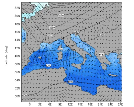
imple-38 1

Figure 2: The 20 October 2011 case study. Geopotential height at 500 hPa (m, 2

black contours) sea surface temperature (°C, filled contours), and surface winds 3

(m/s, vectors plotted every ten grid points). The upper level trough, tilted in the 4

SW-NE direction, and the cyclonic wind at the surface on the lee of the western 5

Alps are well evident. The graph is on 20 October at 00 UTC and is derived from 6

the RAMS output. 7

8 9

Figure 2. The 20 October 2011 case study. Geopotential height

at 500 hPa (m, black contours) sea surface temperature (◦C, filled contours), and surface winds (m s−1, vectors plotted every ten grid points). The upper level trough, tilted in the SW–NE direction, and the cyclonic wind at the surface on the lee of the western Alps are evident. The graph is for 20 October at 00:00 UTC and is derived from the RAMS output.

mented in RAMS, which is the main goal of the paper, with lesser impact of the quality of the model simulation.

3.1 Case of 20 October 2011

The synoptic environment that characterized the storm is briefly discussed. The case study can be classified as a cy-clone developing on the lee of the Alps (Buzzi and Tibaldi, 1978). In particular, an upper-level trough, whose axis was tilted in the SW–NE direction, moved from the UK towards central Europe. In this movement the upper-level winds crossed the western Alps and generated a low-pressure pat-tern at the surface in the Gulf of Genoa.

Moist air masses were advected at lower tropospheric lev-els from the Tyrrhenian Sea toward the Italian mainland. The presence of a low-pressure pattern, the interaction between the moist air masses with the orographic features of Italy, and the presence of the sea–land contrast triggered convection in Italy.

These characteristics of the storm are well represented in the RAMS simulation, as shown in Fig. 2. This figure also suggests the importance of two mesoscale ingredients: (a) the presence of a warm pattern of sea water in the central nian Sea; (b) the convergence of air masses over the Tyrrhe-nian sea in front of Lazio. Both these features have the po-tential to strengthen the convection, the former by injecting water vapour into the overlaying atmosphere, the second by triggering convection along the convergence line.

(7)

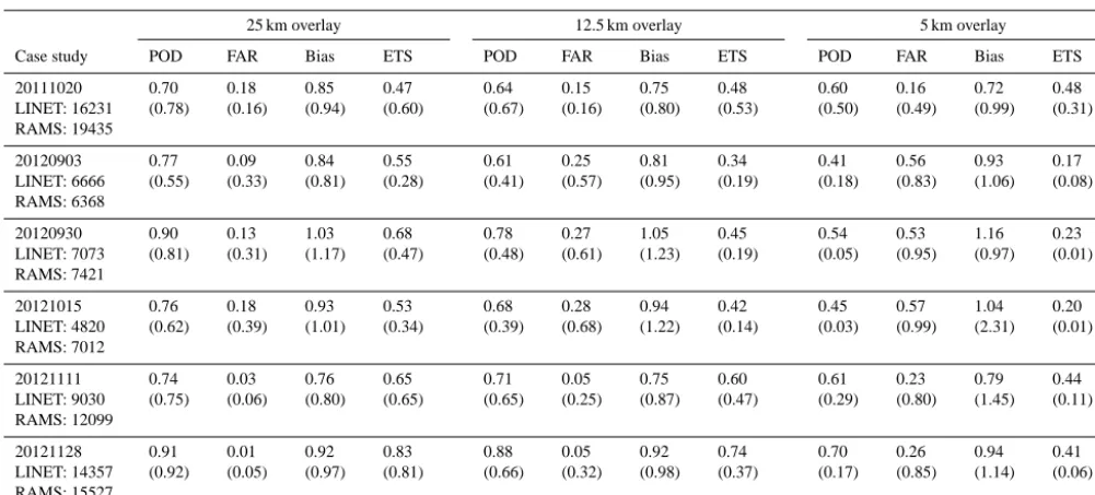
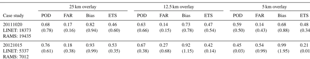
Table 2. Skill score statistics of the six case studies. Date of forecast and number of flashes observed (LINET) and simulated (RAMS) for

each case study are shown in the first column. POD, FAR, Bias, and ETS are given for the MLT1 and MLT10 (in parentheses) for the 25, 12.5 and 5 km overlays superimposed to the 2.5 km RAMS grid. The area considered for the statistics is the area shown in Fig. 4 (10.5–14.5◦E, 40.5–43.5◦N).

25 km overlay 12.5 km overlay 5 km overlay

Case study POD FAR Bias ETS POD FAR Bias ETS POD FAR Bias ETS

20111020 LINET: 16231 RAMS: 19435 0.70 (0.78) 0.18 (0.16) 0.85 (0.94) 0.47 (0.60) 0.64 (0.67) 0.15 (0.16) 0.75 (0.80) 0.48 (0.53) 0.60 (0.50) 0.16 (0.49) 0.72 (0.99) 0.48 (0.31) 20120903 LINET: 6666 RAMS: 6368 0.77 (0.55) 0.09 (0.33) 0.84 (0.81) 0.55 (0.28) 0.61 (0.41) 0.25 (0.57) 0.81 (0.95) 0.34 (0.19) 0.41 (0.18) 0.56 (0.83) 0.93 (1.06) 0.17 (0.08) 20120930 LINET: 7073 RAMS: 7421 0.90 (0.81) 0.13 (0.31) 1.03 (1.17) 0.68 (0.47) 0.78 (0.48) 0.27 (0.61) 1.05 (1.23) 0.45 (0.19) 0.54 (0.05) 0.53 (0.95) 1.16 (0.97) 0.23 (0.01) 20121015 LINET: 4820 RAMS: 7012 0.76 (0.62) 0.18 (0.39) 0.93 (1.01) 0.53 (0.34) 0.68 (0.39) 0.28 (0.68) 0.94 (1.22) 0.42 (0.14) 0.45 (0.03) 0.57 (0.99) 1.04 (2.31) 0.20 (0.01) 20121111 LINET: 9030 RAMS: 12099 0.74 (0.75) 0.03 (0.06) 0.76 (0.80) 0.65 (0.65) 0.71 (0.65) 0.05 (0.25) 0.75 (0.87) 0.60 (0.47) 0.61 (0.29) 0.23 (0.80) 0.79 (1.45) 0.44 (0.11) 20121128 LINET: 14357 RAMS: 15527 0.91 (0.92) 0.01 (0.05) 0.92 (0.97) 0.83 (0.81) 0.88 (0.66) 0.05 (0.32) 0.92 (0.98) 0.74 (0.37) 0.70 (0.17) 0.26 (0.85) 0.94 (1.14) 0.41 (0.06)

2010). It is given by

KI=(T850−T500)+Td850−(T700−Td700) . (7) The KI accounts for the lapse rate (given by the difference be-tween the temperature at 850 hPa,T850, and 500 hPa,T500), for the lower-troposphere moisture content (dew point tem-perature at 850 hPa, Td850), and for the depth of the mois-ture level (estimated by the difference between the temper-ature at 700 hPa,T700, and the dew point temperature at the same level,Td700). The thunderstorm potential for different values of the KI are as follows (Yair et al., 2010): 0 % for 0≤KI≤15; 20 % or unlikely for 18≤KI≤19; 35 % or iso-lated thunderstorms for 20≤KI≤25; 50 % or scattered thun-derstorm for 26≤KI≤29; 85 % or potential of numerous thunderstorms for 30≤KI≤35; 100 % chance of thunder-storms for KI>36.

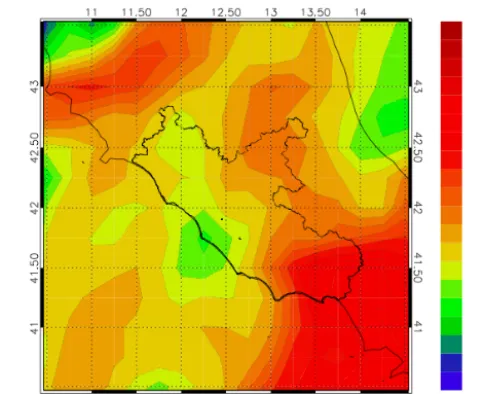
Figure 3 shows the value of the KI derived from the ECMWF operational analysis at 00:00 UTC on 20 October. A wide area over Lazio has KI values larger than 29, showing the potential for numerous thunderstorms occurrence.

Figure 4a shows the lightning density recorded by the LINET on 20 October 2011. The total number of flashes is 16 231 over the whole domain for the whole day, showing an intense electrical activity (the peak is 1521 flashes h−1over the domain). The lightning activity is mainly confined to the west of the Apennines and over the Tyrrhenian Sea, with the largest fraction of flashes occurring between the Apennines and the Sea.

Figure 4b shows the lightning density simulated by apply-ing the methodology described in Sect. 2. The total number

38 1

Figure 2: The 20 October 2011 case study. Geopotential height at 500 hPa (m, 2

black contours) sea surface temperature (°C, filled contours), and surface winds 3

(m/s, vectors plotted every ten grid points). The upper level trough, tilted in the 4

SW-NE direction, and the cyclonic wind at the surface on the lee of the western 5

Alps are well evident. The graph is on 20 October at 00 UTC and is derived from 6

the RAMS output. 7

8 9

Figure 3. KI at the 00:00 UTC on 20 October 2011. The boundaries

of the Lazio Region are also shown.

(8)

2940 S. Federico et al.: Simulating lightning into the RAMS model: implementation and preliminary results

39 Figure 3: KI at the 00 UTC on 20 October 2011. The boundaries of the Lazio 1

Region are also shown. 2

3 4

5 6 7

40 1

2

Figure 4: (a) Flash density (number of flashes per 25 km2 _and_{accumulated over} 3

the whole day) measured by the LINET network on 20 October 2011; (b) Flashes 4

density (number of flashes per 25 km2 _{and accumulated over the whole day)} 5

simulated by applying the DHS method on 20 October 2011. To obtain the flash 6

densities of Figure 4, observed flashes for the whole day have been remapped 7

onto a 5 km x 5 km grid, and the modelled flash density (ρfl) has been integrated 8

over the same grid and for the whole day. Only grid-boxes having at least one 9

flash are shown. The black solid line in Figure 4b shows the latitude of the cross 10

section of Figure 5. 11

12

Figure 4. (a) Flash density (number of flashes per 25 km2and ac-cumulated over the whole day) measured by the LINET network on 20 October 2011; (b) flash density (number of flashes per 25 km2 and accumulated over the whole day) simulated by applying the DHS method on 20 October 2011. To obtain the flash densities of Fig. 4, observed flashes for the whole day have been remapped onto a 5 km×5 km grid, and the modelled flash density (ρfl)has been

in-tegrated over the same grid and for the whole day. Only grid boxes having at least one flash are shown. The black solid line in Fig. 4b shows the latitude of the cross section of Fig. 5.

of occurrence of flashes. This is also evident to the East of the Apennines, where the simulated lightning activity is less than that observed. There are differences (of the order of few tens of kilometres) in the simulated position of the most in-tense convective cells. Nevertheless, the model well repre-sents both the intensity and the position of the lightning ac-tivity over Lazio.

41 1

2

Figure 5: Longitude-height cross section (latitude 41.70 N) at 08 UTC on 20 3

October 2011. Solid contours show areas where graupel density is larger than 0.1 4

g/m3_{(graupel cell); dashed contours show areas where ice density is larger than} 5

0.1 g/m3_{(ice cell). Color filled contours indicate the vertical velocity (m/s). The} 6

height of the 273 K isotherm is roughly indicated. The black mask at the bottom 7

of the figure shows the RAMS orography. 8

9

10

Figure 6: Lightning number (h)-1_{recorded (LINET) and simulated (RAMS) on 20} 11

October 2011 over the domain of Figure 4. 12

13

Figure 5. Longitude–height cross-section (latitude 41.70◦N) at 08:00 UTC on 20 October 2011. Solid contours show areas where graupel density is larger than 0.1 g m−3(graupel cell); dashed con-tours show areas where ice density is larger than 0.1 g m−3 (ice cell). Colour-filled contours indicate the vertical velocity (m s−1). The height of the 273 K isotherm is roughly indicated. The black mask at the bottom of the figure shows the RAMS orography.

41 1

2

Figure 5: Longitude-height cross section (latitude 41.70 N) at 08 UTC on 20 3

October 2011. Solid contours show areas where graupel density is larger than 0.1 4

g/m3_{(graupel cell); dashed contours show areas where ice density is larger than} 5

0.1 g/m3_{(ice cell). Color filled contours indicate the vertical velocity (m/s). The} 6

height of the 273 K isotherm is roughly indicated. The black mask at the bottom 7

of the figure shows the RAMS orography. 8

9

10

Figure 6: Lightning number (h)-1_{recorded (LINET) and simulated (RAMS) on 20} 11

October 2011 over the domain of Figure 4. 12

13

Figure 6. Lightning number(h)−1 recorded (LINET) and simu-lated (RAMS) on 20 October 2011 over the domain of Fig. 4.

To better understand how the lightning scheme works, Fig. 5 shows the vertical distribution of the graupel and ice cells and of the vertical velocity simulated along the 41.70◦N latitude cross-section. The vertical cross-section is at 08:00 UTC, when the simulated convection is at its maxi-mum (see below). There are two graupel cells centred around 12.5 and 13.5◦_{E. Those cells are topped by an ice cell and}

are producing flashes. Within those cells there are two max-ima of the vertical velocity forced by the convection: the first (≈10 m s−1; 12.5◦E–5500 m) inside the main convec-tive cell, the second (≈3.0 m s−1; 13.5◦E–3500 m) in the smaller one.

(9)

42 1

Figure 7: The synoptic environment of the 15 October 2012 case study. 2

Geopotential height at 500 hPa (m, filled contours); sea level pressure (hPa, black 3

contours); surface wind (m/s, vectors plotted every ten grid points). The Figure is 4

on 15 October 2012 at 18 UTC and is derived from the RAMS output. 5

6 7

8 9

Figure 7. The synoptic environment of the 15 October 2012 case

study. Geopotential height at 500 hPa (m, filled contours); sea level pressure (hPa, black contours); surface wind (m s−1, vectors plot-ted every ten grid points). The figure is for 15 October 2012 at 18:00 UTC and is derived from the RAMS output.

the event. In particular, the maximum flash number in 1 h is overestimated by the model (1918 flashes simulated in 1 h compared to 1521 observed) but occurs at the same time (08:00 UTC) as in the observations.

It is worth noting that the comparison shown in this sec-tion between simulated and observed lighting activity is an immediate and powerful tool to assess the model ability to reproduce the intensity and the evolution of the convection.

3.2 Case of 15 October 2012

The synoptic environment in which this storm developed is somewhat similar to that of 20 October 2011. An upper-level trough approached the Mediterranean Basin from NW Europe and interacted with the western Alps. Air masses crossed the western Alps, generating a cyclone on the lee of the Alps (Buzzi and Tibaldi, 1978). This situation is well depicted in the RAMS simulation, Fig. 7, which shows a low pressure on the lee of the Alps (e.g. the 1005 Pa isobar) and a cut-off at 500 hPa. The cyclonic pattern of surface winds ad-vected moist air masses from the Tyrrhenian Sea toward the Italian western coasts, developing convection.

The main difference of this storm compared to the 20 Oc-tober 2011 case study is that the synoptic-scale system moved rapidly to the east and the convection crossed Lazio from north to south in a few hours. The geopotential cut-off at 500 hPa, for example, was centred over NE Italy at 06:00 UTC on 16 October 2012 (not shown).

Figure 8 shows the KI derived from the ECMWF oper-ational analysis at 18:00 UTC on 15 October 2012. Values larger than 29 are shown in the northern part (>42.50◦N) of the domain and in the southern part (<41.50◦N) of Lazio,

42 1

Figure 7: The synoptic environment of the 15 October 2012 case study. 2

Geopotential height at 500 hPa (m, filled contours); sea level pressure (hPa, black 3

contours); surface wind (m/s, vectors plotted every ten grid points). The Figure is 4

on 15 October 2012 at 18 UTC and is derived from the RAMS output. 5

6 7

8

9 _{Figure 8. KI at the 18:00 UTC on 15 October 2012. The boundaries}

of the Lazio Region are also shown.

with a smaller chance of thunderstorms in the central part of the region.

Figure 9a shows the lightning density observed by the LINET network on 15 October 2012. The total number of flashes was 4820 and they occurred mainly in the late after-noon and evening, with a peak of 1319 flashes h−1. From Fig. 9a it is apparent that there is a considerable light-ning activity over the Tyrrhenian Sea, clustered in two main bands of flashes oriented in the southwest–northeast direc-tion, and over the land surface between the Apennines and the sea. However, the comparison of the lightning density registered for the whole day for this and the previous case study (Figs. 5a and 9a) shows that the convection was less intense for 15 October 2012 compared to 20 October 2011.

Figure 9b shows the lightning density simulated using the methodology presented in this paper. The total number of flashes over the domain and for the whole day is 7012 and the model overestimates by 45 % the observed occurrence for this case. Nevertheless, it should be noticed that the model is able to reproduce the less intense lightning activity of this case study compared to the 20 October 2011.

There are two main points to consider from Fig. 9: (a) the lightning activity between the Apennines and the Tyrrhenian Sea is simulated by the model, nevertheless its pattern is shifted to the southeast (O(100 km)) with respect to the ob-servations; (b) the lightning activity over the Tyrrhenian Sea is not well reproduced because the model misses the north-ernmost band of flashes, and the southnorth-ernmost band is mod-elled to the southeast of the observed band.

(10)

43 Figure 8: KI at the 18 UTC on 15 October 2012. The boundaries of the Lazio 1

Region are also shown. 2

3

4

5

44 1

Figure 9: (a) Flash density (number of flashes per 25 km2 _and_{accumulated over}

2

the whole day) measured by the LINET network on 15 October 2012; (b) Flash 3

density (number of flashes per 25 km2 _{and accumulated for the whole day)}

4

simulated by applying the DHS method on 15 October 2012. To obtain the 5

densities of Figure 9, observed flashes for the whole day have been remapped 6

onto a 5 km x 5 km grid, and the modelled flash density (ρfl) has been integrated

7

over the same grid and for the whole day. Only grid-boxes having at least one 8

flash are shown. The black solid line in Figure 9b shows the latitude of the cross 9

section of Figure 11. 10

11

Figure 9. (a) Flash density (number of flashes per 25 km2and ac-cumulated over the whole day) measured by the LINET network on 15 October 2012; (b) flash density (number of flashes per 25 km2 and accumulated for the whole day) simulated by applying the DHS method on 15 October 2012. To obtain the densities of Fig. 9, observed flashes for the whole day have been remapped onto a 5 km×5 km grid, and the modelled flash density (ρfl)has been

in-tegrated over the same grid and for the whole day. Only grid boxes having at least one flash are shown. The black solid line in Fig. 9b shows the latitude of the cross-section of Fig. 11.

of convection in the early hours of the day, which is missed by the model. However, the most intense convective activity occurred, by far, in the late afternoon and evening. RAMS correctly depicts the most intense phase of the convection starting in the afternoon, and the maximum lightning rate oc-curred at 17:00 UTC. Nevertheless, the maximum lightning rate is underestimated by the model (1164 flashes per hour simulated over the whole domain of Fig. 9 compared to 1319

45 1

Figure 10: Lightning number (h)-1_{recorded (LINET) and simulated (RAMS) on} 2

15 October 2012 over the domain of Figure 9. 3

4

5

Figure 11: Longitude-height section (latitude 41.20 N) at 21 UTC on 15 October 6

2012. Solid contours show areas where graupel density is larger than 0.1 g/m3 7

(graupel cell); dashed contours show areas where ice density is larger than 0.1 8

g/m3_{(ice cell). Color filled contours indicate the vertical velocity (m/s). The} 9

height of the 273K isotherm is roughly indicated. The black mask at the bottom of 10

the figure shows the RAMS orography. 11

12 13

Figure 10. Lightning number(h)−1recorded (LINET) and simu-lated (RAMS) on 15 October 2012 over the domain of Fig. 9.

45 1

Figure 10: Lightning number (h)-1_{recorded (LINET) and simulated (RAMS) on} 2

15 October 2012 over the domain of Figure 9. 3

4

5

Figure 11: Longitude-height section (latitude 41.20 N) at 21 UTC on 15 October 6

2012. Solid contours show areas where graupel density is larger than 0.1 g/m3 7

(graupel cell); dashed contours show areas where ice density is larger than 0.1 8

g/m3_{(ice cell). Color filled contours indicate the vertical velocity (m/s). The} 9

height of the 273K isotherm is roughly indicated. The black mask at the bottom of 10

the figure shows the RAMS orography. 11

12 13

Figure 11. Longitude–height section (latitude 41.20◦N) at 21:00 UTC on 15 October 2012. Solid contours show areas where graupel density is larger than 0.1 g m−3(graupel cell); dashed con-tours show areas where ice density is larger than 0.1 g m−3 (ice cell). Colour-filled contours indicate the vertical velocity (m s−1). The height of the 273 K isotherm is roughly indicated. The black mask at the bottom of the figure shows the RAMS orography.

flashes per hour observed), and the event duration is longer compared to the observations. For example, the model is pro-ducing a sizable amount of flashes (548 flashes per hour over the whole domain of Fig. 9) still at 21:00 UTC, when the observations show that the lightning activity is very low (28 flashes per hour over the same domain) and it is ending.

(11)

S. Federico et al.: Simulating lightning into the RAMS model: implementation and preliminary results 2943 the land surface. The vertical velocity shows several local

maxima/minima forced by the convection, but, as expected, their values are lower than those simulated for the 20 Octo-ber 2011 case study (Fig. 5).

Comparing the results of the 15 October 2012 case with those of the 20 October 2011 case it is evident that the sim-ulation is worse for the former case. There are different fac-tors contributing to this result. First it should be noted that the 15 October 2012 case was less intense than other cases considered in this paper, at least over the Lazio Region, and was characterized by weak convective cells, whose simula-tion is difficult because their weak forcing can be missed by the model. For example, the onset of the convection during the night between 14 and 15 October 2012 was caused by small convective cells over the sea and near the coast (not shown, see the discussion paper Federico et al., 2014) that could be likely better simulated by nudging local observa-tions (not available) into the RAMS.

Another important point to remark is that the convergence generated by the model at the surface (Fig. 7), which is a key factor to initiate the convection, is close to the coastline and over the southern part of the Lazio region, where most of the flashes are simulated (Fig. 9b). The development of the convergence zone near the coastline is caused by the flow deflection induced by the orography, which interacts with the undisturbed flow over the sea. The absence of convergence over the sea is a key factor contributing to the missed two bands of flashes over the sea (Fig. 9a).

The misplaced pattern of surface convergence simulated by the model is in turn the result of several factors: (a) ini-tial and dynamic boundary conditions, which can influence the specific model behaviour through the Froude number, or the lack of humidity, or the absence/presence of convergence lines; (b) model deficiencies both physical and dynamical, and; (c) the absence of local observations, which could trig-ger the convective cells.

The above results show also that errors in the simulated microphysical fields are directly transferred to the lightning scheme and to the simulated lightning distribution. This is one of the drawbacks of using the simple lightning scheme adopted in this study.

The results for this case study show that the lightning sim-ulation may be affected by a spatial displacement error of the order of tens of kilometres and by a temporal error of a few hours. It is recognized that these errors are significant from a practical point of view and limit the application of the lightning forecast at finer spatial and temporal scales. Nev-ertheless, they are typical of the current state-of-the-art cold-started cloud-resolving models, as reported in several papers on the subject (McCaul et al., 2009; Yair et al., 2010; DHS2) and as confirmed by the analysis of the objective scores for the other case studies considered in this paper (next section). These errors can be reduced by using data assimilation techniques and, particularly, by the assimilation of lightning data (Fierro et al., 2013; Qie et al., 2013; Lagouvardos et

al., 2013). For example, considering an application over the Mediterranean area, Lagouvardos et al. (2013) used light-ning data from the ZEUS network as a proxy for the pres-ence of convection to control the activation of the convective parametrization scheme in MM5 (Dudhia, 1993). The assim-ilation of lightning proved to have a positive impact on the representation of the precipitation field, particularly of the precipitation maxima, for a heavy precipitation event that af-fected southern France in the period of 6–8 September 2010. It is finally stressed that the displacement in time and space of the simulated lightning activity is an effective diagnostic tool to evidence problems in the forecast of the convection. This shows the importance of using computationally efficient lightning schemes, such as the one described in this paper, in forecast models.

3.3 Scores

To cast the model performance in an objective way, statistical verification was performed by calculating the hits (a), false alarms (b), misses (c), and correct no forecasts (d)for the case studies of 20 October 2011 and 15 October 2012. Start-ing from those statistics, the probability of detection (POD), false alarm rate (FAR), the bias, and the equitable threat score (ETS) were computed (Price et al., 2011; Lynn et al., 2012; Wilks, 2006):

POD= a a+c FAR= b

a+b Bias=a+b a+c ETS= a−ar

a+b+c−ar;ar=

(a+b)(a+c) a+b+c+d ,

wherear is the expected number of correct forecasts in a random forecast where forecast occurrence/non-occurrence is independent of observation/non-observation.

The scores were computed for different grid overlays (35, 25, 12.5 and 5 km grid element size) superimposed to the RAMS grid at 2.5 km resolution for the day considered (24 h), 20 October 2011 and 15 October 2012 respectively. The statistics are presented for the subdomain of the second grid shown in Fig. 4 (10.5–14.5◦E, 40.5–43.5◦N). Two dif-ferent minimum thresholds of lightning events per grid over-lay element are used to compute the scores:≥1 (i.e. a hit is when there is at least one simulated lightning event and at least one registered lightning event in the same grid over-lay element) and≥10 (i.e. a hit is when there are at least 10 simulated lightning events and at least 10 registered light-ning events in the same grid overlay element). Hereafter, these thresholds are referred to as MLT1 (minimum light-ning threshold≥1) and MLT10 (minimum lightning thresh-old≥10).

(12)

46

a)

1

2

b)

3

4

Figure 12: POD (vertical axis) plotted against FAR (horizontal axis) for the 20 5

October 2011 (solid line) and the 15 October 2012 case study (dashed line): a) for 6

MLT1; b) for MLT10. 7

35#km#

25#km# 12.5#km#

5#km# 35#km#

25#km#

12.5#km#

5#km#

0# 0,1# 0,2# 0,3# 0,4# 0,5# 0,6# 0,7# 0,8# 0,9# 1#

0,00# 0,10# 0,20# 0,30# 0,40# 0,50# 0,60#

PO

D$

FAR$

20111020#

20121015#

35#km# 25#km#

12.5#km#

5#km# 35#km# 25#km#

12.5#km#

5#km# 0#

0,1# 0,2# 0,3# 0,4# 0,5# 0,6# 0,7# 0,8# 0,9#

0# 0,2# 0,4# 0,6# 0,8# 1#

PO

D$

FAR$

20111020#

20121015#

Figure 12. POD (vertical axis) plotted against FAR (horizontal axis)

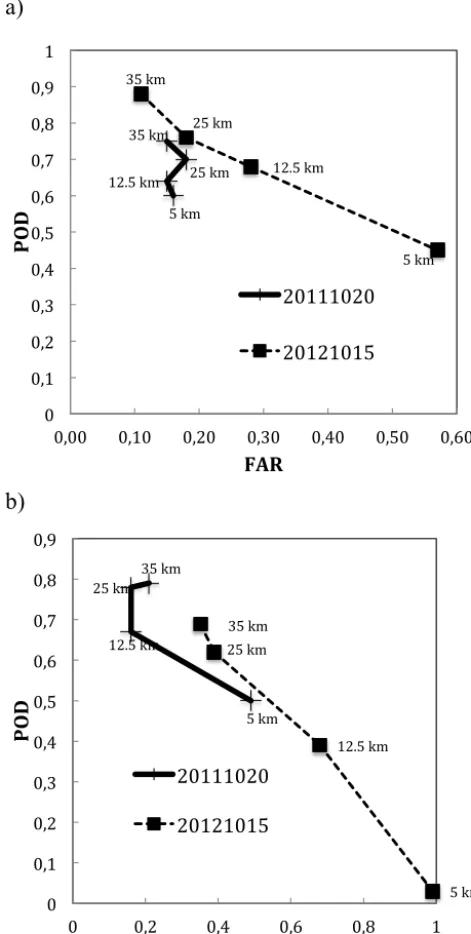
for the 20 October 2011 (solid line) and the 15 October 2012 case study (dashed line): (a) for MLT1; (b) for MLT10.

20 October 2011 (15 October 2012) decreases from 0.75 (0.88) for the 35 km overlay to 0.60 (0.45) for the 5 km over-lay. The FAR is roughly constant (0.16) for the 20 October case, while it increases from 0.11, for the 35 km overlay, to 0.57, for the 5 km overlay, for the 15 October 2012 case. It is noticed that POD is larger than FAR for all grid overlays on 20 October 2011, while POD is less than FAR for the 5 km overlay on 15 October 2012.

The results for the MLT10 are worse. On 20 October 2011 the POD is larger than FAR for all overlays (for the 5 km overlay the POD and FAR are nearly equal), while, on 15 Oc-tober 2012, POD is larger than FAR only for the 35 and 25 km overlays (not for the 12.5 and 5 km overlays). These results show the difficulty of correctly predicting the exact lo-cation of intense convective cells. Similar results were found by Lynn et al. (2012) considering an event in the central US (Tuscaloosa, 27 April 2012). They considered the 36, 12 and 4 km grid overlay sizes superimposed to the 4 km WRF grid (Fig. 8 of Lynn et al., 2012) and found a decrease of the performance for smaller grid sizes and for higher minimum lightning per grid element thresholds. In particular, for the 4 km overlay, the POD was larger than FAR for MLT1, while POD was less than FAR for MLT10.

The statistics of Fig. 12 show, as suggested from the re-sults presented in the previous two sections, that the model performance was better for the 20 October 2011 compared to studies that occurred in fall 2012.

To make the results of this paper statistically more robust, four additional case studies that occurred in fall 2012 are con-sidered. The cases refer to moderate–high lightning activity over Lazio (6666 to 14 357 lightning per day, Table 2) and occurred on 3 September, 30 September, 11 November, and 28 November 2012.

RAMS simulations for these cases were performed using the same grid configuration (Table 1, Fig. 1) as that used for the 20 October 2011 and 15 October 2012 case studies, us-ing the ECMWF operational analysis (0.25◦horizontal res-olution) as initial and boundary conditions. Simulations last 36 h and were initialized at 12:00 UTC on the day preceding the case study (12 h spin-up time). SST was interpolated onto the RAMS grids from ECMWF analyses.

The scores for the 25, 12.5 and 5 km grid overlays, for the whole day of each of the six simulations and for MLT1 and MLT10 are shown in Table 2. Considering the 25 km over-lay, it is noticed that POD is always larger than FAR for both lightning thresholds considered. Considering MLT1, the Bias ranges from 0.76 (11 November 2012) to 1.03 (30 Septem-ber 2012). ETS ranges from 0.47 (20 OctoSeptem-ber 2011) to 0.83 (28 November 2012). The performance decreases for MLT10. The equitable threat score ranges between 0.28 (3 September 2012) and 0.81 (28 November 2012). The Bias ranges between 0.80 (11 November 2012) and 1.17 (30 September 2012).

(13)

47 1

2

Figure 13: Number of grid elements with a number of flashes greater or equal to a 3

given threshold for the 5 km overlay and accumulated over all the case studies. 4

The lightning thresholds are given in the x-axis (1, 5, …, 50 flashes per grid 5

element). 6

7

8

1# 5# 10# 20# 30# 50# RAMS# 7348# 3403# 1657# 590# 293# 111# LINET# 7493# 3115# 1386# 434# 163# 48#

0# 1000# 2000# 3000# 4000# 5000# 6000# 7000# 8000#

#

$o

f$gr

id

$e

le

m

en

ts$

Figure 13. Number of grid elements with a number of flashes

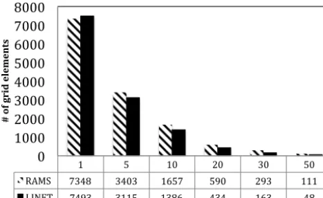
greater than or equal to a given threshold for the 5 km overlay and accumulated over all the case studies. The lightning thresholds are given in thex-axis (1, 5, . . . , 50 flashes per grid element).

to 1.23 (30 September 2012), while the ETS ranges from 0.14 (15 October 2012) to 0.53 (20 October 2011).

For the 5 km overlay the results are worse than for the two larger overlays. However, for the MLT1 the POD is larger than FAR for four cases studies (20 October 2011, 30 September 2012, 11 and 28 November 2012). The Bias ranges from 0.72 (20 October 2011) to 1.16 (30 ber 2012), while the ETS ranges from 0.17 (3 Septem-ber 2012) to 0.48 (20 OctoSeptem-ber 2011). For the MLT10 the POD is always lower than FAR, with the exception of 20 Oc-tober 2011 when POD and FAR show similar values. The Bias ranges from 0.97 (30 September 2012) to 2.31 (15 Oc-tober 2012), while the value of ETS is nearly zero for two case studies (30 September 2012, and 15 October 2012).

Altogether the statistics of Table 2 shows a decrease of the performance of the lightning simulation at finer horizontal scales and for the higher minimum thresholds of lightning events per grid element. This result confirms the findings of other authors and shows the difficulty in correctly simulating the exact position and intensity of the convective cells. It is also stressed that the results of Table 2 quantify objectively that the model had a better performance on 20 October 2011 than on 15 October 2012, and that the cases study presented in detail in the previous two sections span a wide range of model performance as well as of lightning number recorded over the area of study.

It is interesting to consider the performance of the light-ning scheme for other lightlight-ning thresholds. Figure 13 shows the number of grid elements where the simulated lightning number and that recorded by LINET are higher than the MLT value, for different thresholds and for the 5 km overlay. The distributions are obtained by summing over all cases. For the lowest threshold MLT1 (≥1 lightning per grid element), our method underestimates the lightning distribution, which is less spatially extended compared to the observations. This determines a Bias lower than 1.

For the larger thresholds (≥5 lightning per grid element threshold), our method overestimates the observed distribu-tion and it has a larger spatial extension compared to the observations. This determines a Bias larger than 1. This be-haviour is also shown by the results of Table 2.

The same behaviour is obtained for the other grid overlays (not shown) showing a general tendency of the model.

For Fig. 13, however, it should be considered that: 1. it is obtained by summing over all cases and exceptions

to the above results can occur for particular cases; 2. despite that the modelled and observed distributions

may show similar values, the spatial pattern of these dis-tributions can differ, determining low values of ETS and poor prediction. The results for the cases considered in this paper show a decrease of the ETS with increasing thresholds and decreasing grid overlay size.

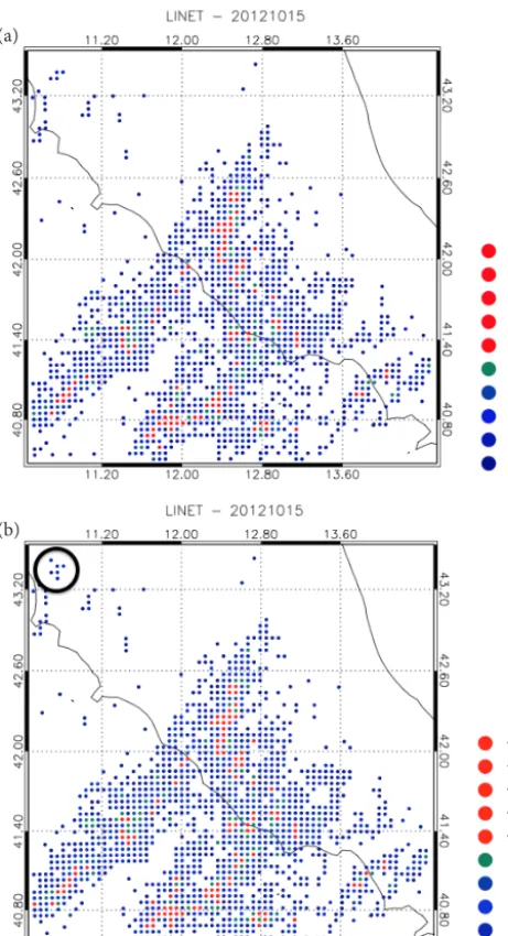
Another point to consider is the impact on the results of the threshold values used for grouping the LINET strokes. In this paper we assumed that all strikes observed within 10 km and 1 s (hereafter R10_1) from an initial strike point are grouped as a single flash. In a recent paper, Yair et al. (2014) showed that using stricter ranges (5 km, 0.5 s, hereafter R5_05) is sufficient to discriminate between successive flashes in most cases.

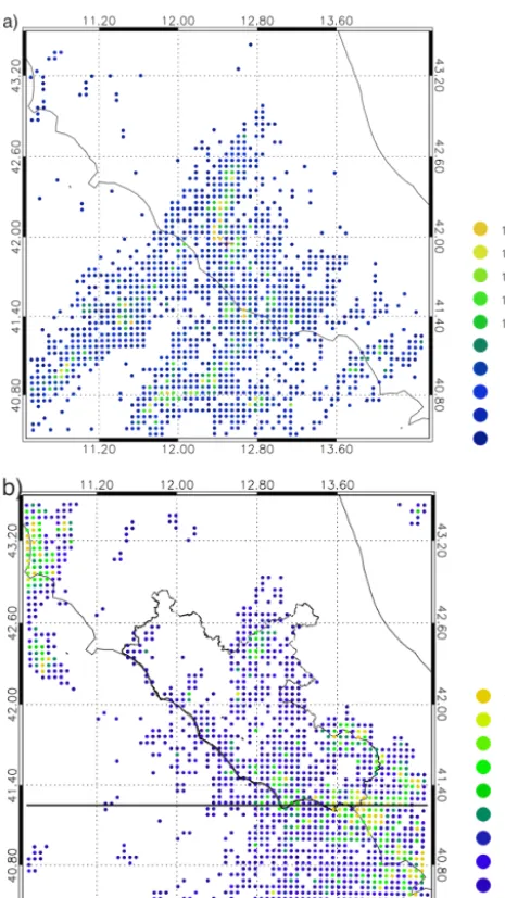
Using R5_05 for the lightning binning affects the results in two ways: (a) by increasing the number of total observed flashes, which spread over a wider area of the verification domain; (b) by increasing the number of grid elements with more than 10 flashes per day. These two effects are apparent in Fig. 14, which shows the flashes for the 15 October 2012 case study for R10_1 and R5_05, respectively.

In particular, the difference between the flashes in the area inside the circle (shown only in Fig. 14b) between R10_1 and R5_05 shows an example of the larger number of flashes obtained for R5_05, while a comparison of the red points in Fig. 14a and b shows the larger number of grid elements having more than 10 flashes per day for R5_05.

Table 3 shows the scores for the 20 October 2011 and 15 October 2012 case studies for R5_05. Comparing the re-sults of Table 2 (R10_1) and Table 3 (R5_05) it can be seen that: (a) the number of lightning is larger for R5_05, as ex-pected; (b) as a consequence of point (a), the bias decreases for R5_05 (particularly for the 15 October 2012 case study for MLT10); (c) the differences between R5_05 and R10_1 are larger as the grid element size becomes finer (i.e. for in-creasing horizontal resolution), because the differences be-tween the observed flashes for R10_1 and R5_05 are small (Fig. 14) and the statistics accounts for this difference when computed at the finer scales; (d) the ETS score shows a small improvement for both cases for R5_05, the largest difference being 0.03 for MLT10 for the 20 October 2011 case study.

(14)

Table 3. Skill score statistics of the 20 October 2011 and 15 October 2012 case study for R5_05 binning ranges. Date of forecast and number

of flashes observed (LINET) and simulated (RAMS) for each case study are shown in the first column. POD, FAR, Bias, and ETS are given for the MLT1 and MLT10 (in parentheses) for the 25, 12.5 and 5 km overlays superimposed to the 2.5 km RAMS grid. The area considered for the statistics is the area shown in Fig. 4 (10.5–14.5◦E, 40.5–43.5◦N).

25 km overlay 12.5 km overlay 5 km overlay

Case study POD FAR Bias ETS POD FAR Bias ETS POD FAR Bias ETS

20111020 LINET: 18373 RAMS: 19435

0.68 (0.78)

0.17 (0.16)

0.82 (0.94)

0.46 (0.60)

0.63 (0.66)

0.14 (0.15)

0.73 (0.78)

0.47 (0.54)

0.59 (0.50)

0.14 (0.43)

0.68 (0.88)

0.48 (0.34)

20121015 LINET: 5337 RAMS: 7012

0.76 (0.61)

0.18 (0.38)

0.93 (0.99)

0.53 (0.35)

0.67 (0.38)

0.27 (0.68)

0.92 (1.15)

0.42 (0.14)

0.45 (0.03)

0.54 (0.99)

0.99 (1.95)

0.21 (0.01)

for R5_05 and for R10_1 for all the cases analysed (not shown, see the discussion paper Federico et al., 2014) as, for example, the better performance of the model for the 20 Oc-tober 2011 case study. This consistency provides further ro-bustness to the findings of this study.

4 Discussion and conclusions

This study shows the application of a new methodology to simulate lightning activity and produce lightning occurrence maps implemented into the RAMS model. The methodology has been applied to six case studies that occurred over the Lazio Region, in central Italy. Two of them were presented in detail. The first one occurred on 20 October 2011, was well represented by the model and was characterized by an intense lightning activity; the second, occurred on 15 Oc-tober 2012, was characterized by moderate lightning activ-ity and was less adequately represented by the model. The number of flashes simulated (observed) over Lazio is 19 435 (16 231) for the first case and 7012 (4820) for the second case. The results show that the model correctly simulates the larger number of flashes that characterized the first event compared to the second.

The analysis of the two cases shows that, particularly on 15 October 2012, there are errors in the timing (O(3 h)) and in the positioning (O(100 km)) of the convection, which are reflected in the simulated spatial and temporal distribution of the flashes.

It is evident that the errors in the simulated convection (timing errors, position error and intensity of convention) are directly transferred to the simulated lightning field. This is the main drawback of the method implemented in this work and in many others reported in the literature. In addition to RAMS deficiencies in the parametrization of the physi-cal processes, initial and dynamic boundary conditions could also play a role and the analysis of the meteorological param-eters at the mesoscale and rapid updated forecasting cycles would very likely mitigate these weaknesses.

A possible way to overcome these limitations in the verifi-cation of the lightning scheme is to restrict the computation

of the scores to those areas where convection is both sim-ulated and observed. This problem was considered in this work, but three main difficulties were encountered: (a) un-availability of the data over the second domain of the RAMS model for some case studies (for example both radar and rain gauges for 11 and 28 November 2012); (b) for some case studies the convection occurred mainly over the Tyrrhenian Sea making the comparison between the model and ground-based data difficult (30 September 2012); (c) less satisfac-tory performance of the model for cases characterized by weak and scattered convection (15 October and 3 Septem-ber 2012). One area where the modelled precipitation was in good agreement with that observed was found for the case study of the 20 October 2011 (not shown, see the discussion paper Federico et al., 2014), and for that area the lightning module gave good results (4318 flashes predicted and 3978 observed). Nevertheless, the direct verification of the light-ning module could not be completely achieved in this work and it will be considered in detail in future studies.

There are drawbacks in the lightning scheme too. As dis-cussed in Sect. 2.2, a simplification of our model is that it considers only two charged regions. Even if the main positive dipole represents the gross structure of thunderstorms (Mac-Gorman and Rust, 1998) with additional charged regions having smaller magnitudes, large thunderstorms exhibit a substantially more complex charge distribution (Stolzenburg et al., 1998) than the single dipole used in our model. This contributes to the discrepancy between modelled and ob-served flashes and its impact is larger for larger thunder-storms.

(15)

47 1

2

Figure 13: Number of grid elements with a number of flashes greater or equal to a 3

given threshold for the 5 km overlay and accumulated over all the case studies. 4

The lightning thresholds are given in the x-axis (1, 5, …, 50 flashes per grid 5

element). 6

7

8

1# 5# 10# 20# 30# 50#

RAMS# 7348# 3403# 1657# 590# 293# 111#

LINET# 7493# 3115# 1386# 434# 163# 48#

0# 1000# 2000# 3000# 4000# 5000# 6000# 7000# 8000#

#$of$grid$elemen

ts$

1

Figure 14: Flashes observed for the 15 October 2012 case study: a) choosing 2

larger ranges (10km , 1 s) for binning the strokes from an initial strike point 3

recorded by LINET; b) as in a) but choosing stricter ranges (5km , 0.5 s). 4

Observed flashes for the whole day have been remapped onto a 5 km x 5 km grid 5

superimposed to the RAMS grid. The red dots show the grid elements with more 6

than 10 flashes for the whole day. 7

8

(a)

(b)

Figure 14. Flashes observed for the 15 October 2012 case study: (a) choosing larger ranges (10 km , 1 s) for binning the strokes from

an initial strike point recorded by LINET; (b) as in (a) but choosing stricter ranges (5 km, 0.5 s). Observed flashes for the whole day have been remapped onto a 5 km×5 km grid superimposed to the RAMS grid. The red dots show the grid elements with more than 10 flashes for the whole day.

and negative cloud-to-ground and intracloud) were properly taken into account by considering their specific characteris-tics (currents, threshold energy for the discharge, etc.).

Another drawback of the lightning scheme is that all the energy accumulated in the plane capacitor is converted to flashes in a single application of the lightning scheme. Lynn et al. (2012) showed the importance of the advection of the electric potential energy from one grid-cell to another as a producer of lightning.

Assuming a constant lightning efficiency (γ=0.9) through the lifetime of the storm is another source of error of the lightning model. The lightning efficiency describes the contribution from lightning to the total discharging of the ca-pacitor, but other effects such as corona currents and pre-cipitation currents might contribute to the discharge. To our knowledge, no exact estimates of the relative contributions of these effects in the different stages of evolving storms exist. The lightning efficiency, however, was included to account for these effects, and it can be adjusted as new research will quantify more precisely the behaviour of this parameter in the different stages of the convection.

The lightning model adopted in this paper assumes fixed polarities of the capacitor plates (i.e. the upper plate is pos-itively charged while the lower plate is negatively charged). Clouds with the main dipole inverted, as those observed by Rust el al. (2005), cannot be handled by this scheme. A pos-sible way to overcome this limitation would be the assump-tion of a reversed polarity for clouds showing some specific characteristics. This issue will be explored in future studies.

Despite these issues, which contributed to cause discrep-ancy between observed and measured lightning activity, sta-tistical scores show objectively the ability of the methodol-ogy implemented in this paper to simulate the daily lightning activity for several spatial scales and for two different mini-mum thresholds of lightning events per grid element.

An advantage of using the methodology presented is that it is simple to implement and computationally fast. It takes 5 s of a state-of-the-art desktop computer to elaborate once the lightning scheme for both domains of Fig. 1. This is impor-tant for several applications, based on nowcasting and short-term forecasting of the lightning activity, such as ground ser-vice planning in airports or in general for outdoor activities where public safety could be affected by lightning. More-over, our scheme, being based on the ice and mixed-phase hydrometeors simulated by RAMS is more physically based compared to the methods using thermodynamic indices, as shown by several studies (Petersen et al., 2005; Katsanos et al., 2007a; Yair et al., 2010).

Besides future studies dedicated specifically to solve some critical issues of our methodology, there are at least two main directions for future development of the research presented in this paper:

1. the use of lightning data assimilation to improve the forecast in time and space of the convective activity, es-pecially its triggering over the sea;

2. the improvement of the physics and dynamics of the model should improve its microphysical fields and the derived lightning activity.

Finally, the lightning simulation presented in this paper can be exploited in an ensemble system, using a similar approach to that described in Federico et al. (2008), based on the comparison between model pseudo water vapour images and