RESEARCH
Constrained incremental tree building: new
absolute fast converging phylogeny estimation
methods with improved scalability and accuracy
Qiuyi Zhang
1, Satish Rao
2and Tandy Warnow
3*Abstract
Background: Absolute fast converging (AFC) phylogeny estimation methods are ones that have been proven to recover the true tree with high probability given sequences whose lengths are polynomial in the number of number of leaves in the tree (once the shortest and longest branch weights are fixed). While there has been a large literature on AFC methods, the best in terms of empirical performance was DCMNJ, published in SODA 2001. The main empiri-cal advantage of DCMNJ over other AFC methods is its use of neighbor joining (NJ) to construct trees on smaller taxon subsets, which are then combined into a tree on the full set of species using a supertree method; in contrast, the other AFC methods in essence depend on quartet trees that are computed independently of each other, which reduces accuracy compared to neighbor joining. However, DCMNJ is unlikely to scale to large datasets due to its reli-ance on supertree methods, as no current supertree methods are able to scale to large datasets with high accuracy. Results: In this study we present a new approach to large-scale phylogeny estimation that shares some of the fea-tures of DCMNJ but bypasses the use of supertree methods. We prove that this new approach is AFC and uses polyno-mial time and space. Furthermore, we describe variations on this basic approach that can be used with leaf-disjoint constraint trees (computed using methods such as maximum likelihood) to produce other methods that are likely to provide even better accuracy. Thus, we present a new generalizable technique for large-scale tree estimation that is designed to improve scalability for phylogeny estimation methods to ultra-large datasets, and that can be used in a variety of settings (including tree estimation from unaligned sequences, and species tree estimation from gene trees). Keywords: Phylogeny estimation, Short quartets, Sample complexity, Absolute fast converging methods, Neighbor joining, Maximum likelihood
© The Author(s) 2019. This article is distributed under the terms of the Creative Commons Attribution 4.0 International License (http://creat iveco mmons .org/licen ses/by/4.0/), which permits unrestricted use, distribution, and reproduction in any medium, provided you give appropriate credit to the original author(s) and the source, provide a link to the Creative Commons license, and indicate if changes were made. The Creative Commons Public Domain Dedication waiver (http://creat iveco mmons .org/ publi cdoma in/zero/1.0/) applies to the data made available in this article, unless otherwise stated.
Introduction
The inference of phylogenies from molecular sequence data is generally approached as a statistical estimation problem, in which a model tree (equipped with a model of sequence evolution) is assumed to have generated the observed data, and the properties of the statistical model are then used to infer the tree. Various statistical approaches can be applied for this estimation, including maximum likelihood, Bayesian techniques, and methods
that operate by computing a distance matrix and then computing the tree from the distance matrix.
Many stochastic sequence evolution models have been developed, starting with the Cavender–Farris–Neyman [1, 2] symmetric two-state model (referred to henceforth as “CFN”) and including increasingly complex molecu-lar sequence evolution models (with four states for DNA, 20 states for amino acids, and 64 states for codon sequences). However, typically the theory that can be established under the CFN model can also be established under the more complex molecular sequence evolution models used in phylogeny estimation.
Under standard sequence evolution models, many methods are known to be statistically consistent
Open Access
*Correspondence: [email protected]
(meaning that they will provably converge to the true tree as the sequence lengths increase), including maxi-mum likelihood [3] and many distance-based meth-ods [4, 5]. However, with the increasing availability of sequence datasets (e.g., the SILVA database has sev-eral million RNA sequences [6]), the need for phylog-eny estimation methods that can be highly accurate on ultra-large datasets has increased. Therefore, a key challenge is to have methods that can scale to large datasets while maintaining good accuracy. Hence, the most desirable methods are those that run in polyno-mial time and that recover the true tree with high prob-ability from short sequences (i.e., sequences that do not have very many sites). In this respect, methods that are “absolute fast converging” [7–9] (i.e., methods that recover the true tree with high probability from poly-nomial length sequences) are the most promising.
There are several methods that have been established to be absolute fast converging (AFC) under the CFN model, including maximum likelihood [3] (if solved exactly) and various distance-based methods [7–14]. Some of these algorithms achieve a poly-logarithmic sample complexity but require a balanced model tree and an upper bound on g, the maximum edge weight (defining the expected number of changes of a random site) in the CFN model. Specifically, methods based on reconstruction of ancestral sequences provide the best sample complexity bounds but cannot handle the case where g is larger than what is known as the Kes-ten–Stigum threshold, which is ln(√2) [15] for the CFN model. The “short quartet” methods were the earliest AFC methods (which are AFC in the regime where g is unbounded), but these are designed to either return the true tree or else fail to return anything [7–9].
Two of the fastest AFC methods are the Harmonic Greedy Triplets (HGT + FP) method by Csűrös [16] and a method developed by King et al. [17]; these meth-ods use O(n2) time and are based on quartet trees, and have the desirable property that they always return a tree for every input. Another good approach is DCMNJ,
which uses a divide-and-conquer technique [9]. In the first phase, O(n2) trees are computed, each based on dividing the sequence dataset into overlapping subsets, constructing trees on each subset using the polynomial time distance-based method neighbor joining (NJ) [18], and then combining the subset trees using a supertree method. This approach differs from other AFC methods in its use of neighbor joining to construct trees on sub-sets, whereas the other AFC methods in essence con-struct the tree by independently concon-structing quartet trees, and then assembling the quartet trees together using a quartet amalgamation method.
Very few AFC methods have been implemented; how-ever, a study [10] comparing HGT+FP [16] and DCMNJ [9]
showed that DCMNJ had better accuracy. Since the theory
does not predict this, the results on simulated data sug-gest that the use of NJ to construct trees on subsets and
then combine the trees using a supertree method may be empirically advantageous compared to methods that combine quartet trees that are estimated independently. Unfortunately, the reliance on a supertree method to combine subset trees means that DCMNJ is unlikely to
scale to ultra-large datasets, because no current supertree method has shown the ability to maintain good accuracy and reasonable running times on large datasets [19].
The purpose of this paper is to describe a new polyno-mial time AFC phylogeny estimation method that should improve on DCMNJ: it is designed to have comparable
accuracy to DCMNJ but also to be able to analyze
ultra-large datasets (i.e., more than 100,000 sequences). The basic approach of this new method is similar to DCMNJ
in that it uses divide-and-conquer, applies neighbor join-ing to subsets of the sequence dataset, and then merges the subtrees together. However, it differs from DCMNJ in
a few important ways, which we describe below. Most importantly, it divides the taxon set into disjoint subsets and then merges the subset trees without relying on any supertree method; thus, it avoids the challenge of relying on existing supertree methods, none of which are likely to scale to large datasets. We present the results here initially for the CFN model, and then extend the results for the Generalized Time Reversible (GTR) model [20]. Our arguments for correctness are very similar to those in [16, 17].
Background material
Absolute fast convergence under the CFN model
Under the Cavender–Farris–Neyman (CFN) model, we have a rooted binary tree T and substitution probabili-ties p(e) on the edges e of T. The state at the root is 0 or 1 with equal probability, and the state changes on edge e
with probability p(e), with 0<p(e) <0.5 for all edges e.
This model can be used for sequence evolution by requir-ing that all the sites evolve i.i.d. down the tree. Finally, we define w(e)= −12log(1−2p(e)). We also define CFNf,g
to be the set of all CFN model trees (T,�) (where
denotes the set of numeric parameters on the edges) with
f ≤w(e)≤g for all edges in T, for arbitrarily selected
positive real numbers f ≤g.
Definition 1 A phylogeny estimation method is said to be absolute fast converging (AFC) under the CFN model if, for all positive values f,g,ǫ (with f ≤g ), there
topology T given sequences of length p(n) with probabil-ity at least 1−ǫ. Note that the polynomial will in general
depend on f, g and ǫ.
DCMNJ+ SQS: an AFC method with good empirical
performance but low scalability
Here we describe the approach used in [9] called “DCMNJ+ SQS”, which was shown to have high
accu-racy in simulation studies with up to 1600 sequences [10]. (Note: “DCM” refers to “disk-covering method” and “SQS” refers to the “short quartet support” crite-rion; see [5, 9]). The input is a set of sequences gener-ated by an unknown model tree and a dissimilarity matrix d (i.e., a symmetric matrix that is zero on the diagonal) where dij is the estimated distance between taxa si and sj, based on the selected sequence
evolu-tion model. For example, when the model is CFN, then dij= −12ln(1−2Hij) will be the “empirical CFN
distance”, where Hij is the Hamming distance between
sequences i and j divided by the sequence length (i.e., the normalized Hamming distances). Note that these empirical CFN distances converge in probability to
Dij= −12log(1−2Eij) where Eij is the expected nor-malized Hamming distance between sequences in leaves i and j, and that D is an additive matrix for the model tree. DCMNJ+SQS uses a two-phase structure, as
follows.
• Phase 1: A set T of O(n2) trees is computed, with at
most one tree tq for each entry q in the dissimilarity matrix d.
• Phase 2: All the trees in T are scored using the SQS criterion (where “SQS” refers to the short quartet support, defined in [9]) and the best-scoring tree is returned.
Before we can describe these phases, we need to provide some definitions.
Definition 2 (From [21]) For the given dissimilar-ity matrix d and positive real number q, we define the threshold graph TG(d, q) to be the graph with the n taxa as the vertex set and edges (i, j) if and only if dij≤q.
We also assign weight dij to each edge (i, j) in TG(d, q). Hence, TG(d,∞) denotes the complete graph with edge weights given by the dissimilarity matrix d.
We use a standard technique, called the Four Point Method, to compute quartet trees (i.e., unrooted binary trees on four leaves) that is based on the Four Point Con-dition [22].
Definition 3 (From [7]) Given a four-taxon set
{u,v,w,z} and a dissimilarity matrix d, the Four Point
Method ( FPM ) infers tree uv|wz (meaning the quar-tet tree with an edge separating u, v from w, z) if d(u,v)+d(w,z)≤min{d(u,w)+d(v,z),d(u,z)+d(v,w)}.
If equality holds, then the FPM infers an arbitrary topology.
Phase 1 for DCMNJ+SQS is performed as follows.
Given q (the selected threshold), the threshold graph
TG(d, q) is computed, then edges are added to the graph to make it triangulated (if necessary), where a triangu-lated graph is one that has no simple cycles of size four or more; furthermore, if d is additive, then TG(d, q) is triangulated. Once the triangulated graph is computed, the set of all maximal cliques can be extracted in poly-nomial time. See [9] for additional details and proofs.
Trees are computed for each maximal clique using neighbor joining [18], and the trees on these cliques are then combined into a tree on the full set of species using a selected supertree method. Phase 2 uses the
SQS criterion, but other criteria also have good theo-retical properties. The SQS score of a tree T, defined by SQS(T), is the maximum l such that for all quartets
{u,v,w,x} of taxa with maximum interleaf distance at
most l, the Four Point Method on {u,v,w,x} produces a
four-leaf tree that agrees with the T.
Theorem 1 (From [9, 10]) The short quartet sup-port (SQS) criterion score can be calculated for each treetq∈T in polynomial time. Also, there is a polyno-mialp(n)such that ifT contains the true treeTand the sequences are of length p(n) (where n is the number of leaves), then with probability at least1−ǫ,the tree inT with the highest SQS score is the true treeT.
The basic approach has good theoretical guarantees (i.e., it is AFC, and more generally if X is any
exponen-tially converging base method (meaning X recovers the
tree with high probability given exponentially many sites) and Y is any true tree selection criteria that has
the same theoretical properties as SQS (as given in Theorem 1), then DCMX+Y is AFC. Empirical
perfor-mance of DCMNJ+SQS on simulated data was excellent,
substantially outperforming NJ and fast
triplet/quartet-based greedy tree growing methods, such as HTP+FP,
on large datasets especially when there was a high rate of evolution [10]. However, these studies were lim-ited to datasets with at most 1600 sequences. In other words, DCMNJ+SQS was not tested on very large
Furthermore, the design of DCMNJ suggests some
limita-tions in terms of scalability to large datasets. Most impor-tantly, supertree methods do not have good scalability, as all current supertree methods with good accuracy are attempts to solve NP-hard optimization problems, and so become computationally intensive on large datasets [19]. Hence, any reasonably fast method will need to com-pletely avoid the supertree calculation step.
Incremental tree‑building ( INC)
We begin by describing the INC method in the uncon-strained condition (i.e., when there are no constraint trees), and prove that it is AFC.
High‑level description of INC
The input to INC is a dissimilarity matrix d. We pre-sent a high-level description of how tree t=INC(d) is computed.
• Find the insertion ordering σ=x1,x2,. . .,xn. • Initialize t as the three-leaf tree on the first three taxa
in the ordering. • For i=4 up to n.
• Determine the set of valid quartets to use for plac-ing xi into tree t.
• Compute quartet trees for each valid quartet, and let them vote for where to place xi.
• Pick the edge e in t that has the most votes; if this is a tie, pick an edge at random from the set of edges with the most votes.
• Insert xi into edge e.
• Return the resulting tree t.
Thus, at a high-level, the INC algorithm operates by greedily growing a tree t based on a computed sequence addition ordering. Yet, many of the details of the algo-rithm are unspecified (e.g., we do not say how we calcu-late the insertion ordering, how we determine the set of valid quartets, how we compute trees on valid quartets, and how the quartet trees vote). Below, we provide details for each of the steps for this algorithm.
Computing the sequence addition ordering
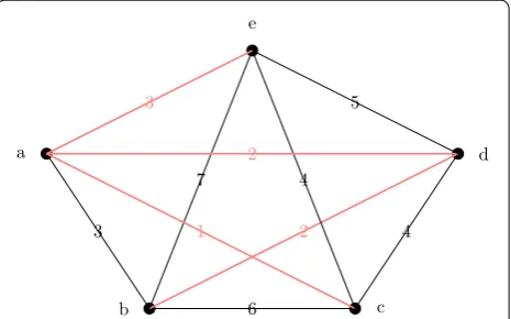
We begin by constructing a minimum spanning tree S of TG(d,∞), where d is the input dissimilarity matrix. Once
the spanning tree S is computed, we choose an arbitrary leaf in S to be the starting vertex in the ordering. Then we order the vertices according to order of traversal in a
BFS (or DFS) from the starting vertex. See Fig. 1 for an example.
How we compute the growing tree t
We initialize our tree t by choosing the first three taxa according to our insertion ordering and forming the three-leaf tree with an internal node that connects to all three taxa. In order to define how we insert the remaining taxa into t, we need to formally define the “valid quartets” and how we compute quartet trees for valid quartets.
Definition 4 Let q0 be the maximum weight of an edge
in S and let q=8q0, A quartet of leaves is valid if its
max-imum pairwise distance (i.e., diameter) is at most q. The quartet tree for the valid quartet is computed using the Four Point Method.
As we will show later, the restriction to just the “valid quartets” allows us to develop a tree construc-tion method that runs in polynomial time and that is AFC. Note also that restricting the diameter of the valid quartets to small values has a mixed effect: if the maxi-mum permitted diameter is too small then even cor-rect quartet trees will not be sufficient to reconstruct the tree, but if the maximum permitted diameter is too large then some computed quartet trees are more likely to be incorrect. We show that this setting for the max-imum diameter q to be 8q0 is sufficient to allow us to
prove that the algorithm is AFC. However, we did not try to optimize this constant, and hence the choice of the constant 8 is likely not optimal (i.e., smaller con-stants might give better theoretical results).
There may be many valid quartets, but we only need to examine a linear number of these, as we now show. Suppose we wish to add a vertex x into t. Given an internal node u of t, because t is binary the removal of
u splits t into three non-empty components which we
a
b c
d e
6
3 2
7
1 4
4 2
3 5
Fig. 1 How the insertion ordering is computed. We show the threshold graph TG(D,∞) and a minimum spanning tree S in red. A possible insertion ordering produced by a BFS on S starting at e is
will refer to as t1,t2,t3 (with internal nodes included).
Because the leaves of t form a connected induced sub-tree of S, we can find taxa ui in ti and vi ∈V(t)\ti such that (ui,vi) is an edge in S, for i=1, 2, 3. We will
associ-ate the triplet u1,u2,u3 to node u, so that the addition
of leaf x defines a quartet, and we can check to see if the quartet is valid. We summarize this discussion with the following definition.
Definition 5 Let u be an internal node of a binary tree
t and let u1,u2,u3 be leaves in the three components of t upon removing u such that there exists vi with (ui,vi)
an edge in S where vi is not in the same component as ui. Then, for some choice of q∈R+, a quartet query on
{u1,u2,u3,x} is q-valid iff the d-diameter (maximum
pairwise distance with respect to the input matrix d) of
{u1,u2,u3,x} is less than q. We use the term valid when q
is clear from context.
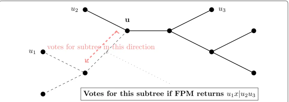
To determine how to place leaf x into the growing tree
t, we compute a tree for each valid quartet query (which includes x) using the Four Point Method. For example, if the tree computed on valid quartet query u1,u2,u3,x
(with ui∈ti, and t1,t2,t3 the three subtrees off internal
node u) returns xu1|u2u3, then this implies that x should
be placed in the subtree of t induced on t1∪u hence,
each edge in that subtree will receive a vote (Fig. 2). Thus, each valid quartet adds a vote to each edge in some non-empty subtree of the tree. We define the sup-port of an edge in the tree t to be the number of valid
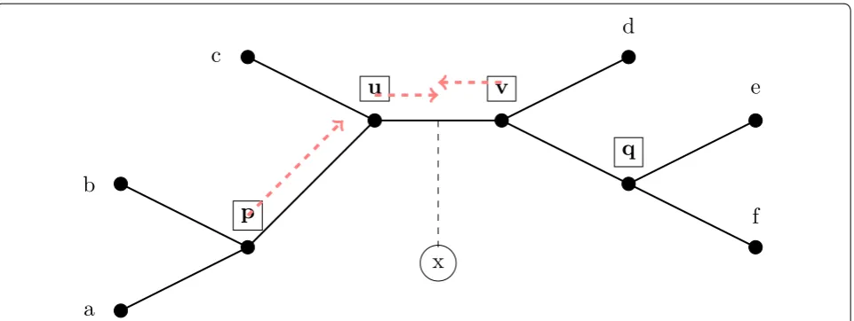
quartet trees that voted for that edge. We then choose an edge e in the tree t that has the largest total support (and if there is a tie, we pick an edge e at random with the maximum support). We then subdivide e and then make x adjacent to the node created. See Fig. 3 for an illustration of how this voting procedure operates.
Furthermore, as we will shortly show, when the sequences are long enough, then there will be a unique edge on which all queries agree, and so the algorithm will correctly add x into t (in such a way that it agrees with the model tree T), and so inductively the greedy algorithm will construct the model tree.
Theoretical properties of INC under the CFN model
We now establish the theoretical properties of AFC
under the CFN model. Throughout this section, recall that dij is the empirical CFN dissimilarity between
taxa i, j and Dij is the underlying CFN model distance
between taxa i, j defined by the model tree (T,�) with edge weights given by w(e)= −12log(1−2p(e)).
Given matrices d and D and positive real q, we define
ǫ(q)=max{|dij−Dij| :dij ≤qorDij≤q}.
Theorem 2 Letdbe a dissimilarity matrix, Dan addi-tive matrix defining a model tree T with edge weights w:E(T)→R+,andq=8q0,whereq0is the maximum distance in the minimum spanning tree ofTG(d,∞).Let
fbe the weight of the shortest internal edge inTand sup-poseǫ(q) <f/2andq0≥f/2,thenINC(d)returnsT.
u
1u
2u
3u
Votes for this subtree if FPM returns
u
1x
|
u
2u
3votes for subtree in this direction
Proof We proceed by induction on the number of leaves in T. Our claim holds when T has three leaves, since there is only one such topology. Let t be the tree maintained by INC before the insertion of the last taxon
x according to our insertion ordering. By induction, t
must have the correct topology. It suffices to show that valid queries can determine the accurate placing of x. Assume that the correct location on which to place x is
e=(u,v) of t. Note that when ǫ(q) <f/2, the Four Point Method is guaranteed to correctly construct quartet trees for all quartets with diameter at most q (and hence for all valid quartets), so that all valid node queries will return the correct quartet tree. Therefore, e will receive all possible votes.
To show that all other edges will miss at least one vote, it suffices to show that node queries are valid at u and v
because all other edges will miss a vote from one of the two such queries, confirming that x is inserted at e (if one of u, v is a leaf vertex, the same conclusion is achieved).
We will show that a node query at u is valid; a similar argument is done for v. Let u1,u2,u3 be selected upon the
deletion of u with their corresponding vi. First, for all i,
D(ui,vi)≤q0+f/2 since d(ui,vi)≤q0 and ǫ(q)≤f/2.
Then, since vi∈V\ti and t is the correct tree topology,
D(ui,u)≤D(ui,vi)≤q0+f/2, where D is the true
dis-tance matrix and u is the corresponding internal node in
T.
Next, we claim that D(x,u)≤2q0+f and together
we will have concluded that {u1,u2,u3,x} is a quartet of d-diameter at most 3q0+2f since by triangle
inequal-ity, we deduce {u1,u2,u3,x} is of D-diameter 3q0+3f/2
and so the d-diameter is bounded at 3q0+2f ≤7q0≤q,
proving validity.
For the last claim, since x is within q0 of some leaf x′
in t, D(x,x′)≤d(x,x′)+f/2≤q0+f/2. Since the path x to x′ must pass through u or v in T and e=(u,v) is the correct edge insertion location, we conclude that
min(D(x,u),D(x,v))≤q0+f/2.
If D(x,u)≤q0+f/2, then our claim follows (we
auto-matically get D(x,u)≤2q0+f ). Else, D(x,v)≤q0+f/2.
Since v∈V(t3),D(x,u)≤D(x,v)+D(u,v)≤q0+f/2+ D(u,v)≤q0+f/2+D(u,u3)≤q0+f/2+q0+f/2≤
≤2q0+f.
Therefore, if the correct edge is (u, v), then the query at u votes against all edge placements for x in t1∪t2, and
symmetrically for v. Hence all other edges will miss at
least one vote.
Theorem 3 Given then×ndissimilarity matrixdand a givenq,INC(d)can be implemented inO(n2)time and
space.
Proof It suffices to show that as we grow our tree t, each insertion step can be implemented to take O(n) time. First, each internal node, when initialized due to an inserted taxon, can store the necessary vertices u1,u2,u3
and that can be done in O(n) time. Each node query is
O(1), so in total the |V(t)| node queries take O(n) time. The only possible difficulty is efficiently finding the edge with the most votes. A naive implementation will lead to an O(n3) runtime. For any edge e=(u,v) on the tree, let n(e) denote the total number of votes that e has.
u
v
p
q
x
a
b
c
d
e
f
Fig. 3 Using quartet queries to place new taxa. When adding a taxon x into the tree t, all valid quartet queries are allowed to vote for the edges in the tree (see Fig. 2) and x is then added to the edge that receives the most votes. In this figure, we show x being placed into edge uv, based on the following possible vote outcomes: The query at p returns tree ab|xc and so votes for {pu,uc,uv,vd,vq,qe,qf}, and similarly the queries at u and
Note that if e,e′ are adjacent edges in t with common
vertex u, then n(e)−n(e′) can be determined by simply looking at the short quartet query at u. Specifically, let
e=(u,v) and e′=(u,v′) be adjacent edges at vertex u. If the query at u was invalid or it showed that x should be in tj with v,v′�∈tj, then n(e)−n(e′)=0. Otherwise, if the query returned tj with v∈tj, then n(e)−n(e′)=1; a sim-ilar argument shows that if v′∈tj then n(e)−n(e′)= −1.
Therefore, by using this local property, we can calculate n(e)+C for some constant C in O(n) time by performing
BFS starting from any leaf of the tree. The BFS then
sim-ply returns the edge with the highest score.
Finally, throughout the algorithm, we need to store the dissimilarity matrix, spanning tree, insertion ordering, and O(1) vertices at each node of the tree. Together, this
requires O(n2) space.
Theorem 4 (Azuma’s inequality [23]) Suppose X=(X1,X2, ...,Xk) are independent random variables
taking values in any set S, and letL:Sk →Rbe any func-tion that satisfies the condifunc-tion:|L(u)−L(v)| ≤t
when-ever u and v differ in just one coordinate. Then,
Theorem 5 For k =�
ln(n/ǫ)e4q
f2
, with probability
≥1−ǫ, we have ǫ(q) <f/2. Furthermore, if q0 is the minimum value ofqsuch thatTG(d, q) is connected, then q0=O(glogn)andq0≥f/2.
Proof To show that ǫ(q) <f/2, we must show that |Dij−dij|<f/2 when Dij <q or dij <q. First, if Dij <q
we show that k=�
ln(n/ǫ)e2q
f2
suffices to show
|Dij−dij|<f/2 holds with probability ≥1−ǫ/n2. We
express our probability of failure as:
The first expression can be written as:
P(|L(X)−E[L(X)]| ≥)≤2 exp
−
2
2t2k
P(|Dij−dij| ≥f/2)=P
log
1−2Hij
1−2Eij ≥ f
≤P((1−2Eij)e−f ≥1−2Hij)+P(1−2Hij≥(1−2Eij)ef)
P(Hij−Eij ≥ 1 2(1−e
−f)(1
−2Eij))
≤P(|Hij−Eij| ≥ 1 2(1−e
−f)e−2Dij)
≤2 exp(−�(k(1−e−f)2e−4q)) ≤2 exp(−�(lnn/ǫ))
The second line follows from Azuma’s (Theorem 4) with
t=1/k. Similarly, the second expression is equivalent to:
Next, if dij<q, then we show that Dij<2q+1 with high probability and then apply the previous result with
q′=2q+1. First, if we let rij=Dij−q, then by simple algebra our probability that dij<q when rij >q+1 is bounded by
The fourth to fifth line follows since e2rij−1> 12e2rij
whenever rij>1. Therefore, by a union bound, we
con-clude our claim that ǫ(q) <f/2 with probability ≥1−ǫ.
We now show that q0=O(glogn). Note that in our
model tree, since g is the maximum weight of an edge in a binary tree with n leaves, it follows that TG(D,O(glogn)) is connected. By our previous part, we know that
|dij−Dij|<f/2 for all edges in TG(D,O(glogn)).
There-fore, we conclude that TG(d,O(glogn)) is also con-nected, and so q0=O(glogn).
Lastly, we show q0≥f/2. Consider all edges in the minimum spanning tree of TG(d,∞). These edges have true weight (in D) at least f and by our previous part the weight of the edges in the minimum spanning tree devi-ate from the true weight (as defined by the model tree) by at most f / 2. Thus, we conclude that q0≥f/2.
Theorem 6 INCis absolute fast converging for the CFN model and takes O(n2) time and space (assuming
dis-tances are precomputed).
Proof All we need to establish is that for every triplet
ǫ,f,g with 0<f <g<∞ and ǫ >0, there is a
polyno-mial p(n) such that for all model trees (T,�) in CFNf,g, P(Eij−Hij ≥
1 2(e
f −1)(1−2E ij))
≤P(|Eij−Hij| ≥ 1 2(e
f
−1)e−2Dij)
≤2 exp(−�(k(ef −1)2e−4q))
≤2 exp(−�(lnn/ǫ))
P(dij<q)=P(Dij−dij >Dij−q)
=P
−1
2log
1−2Eij
1−2Hij
>Dij−q
=P(1−2Hij >e2rij(1−2Eij))
=P
Eij−Hij>
1 2(e
2rij−1)e−2Dij
=P
|Eij−Hij|>
1 4e
2rij−2Dij
≤2 exp(−�(ke−4q))
given sequences of length at least p(n) generated by (T,�) and empirical CFN dissimilarity matrix d com-puted on these sequences, the tree returned by INC(d) is the model tree T with probability at least 1−ǫ.
Let q be the maximum edge weight on the mini-mum spanning tree in the underlying model tree. We know q=O(glogn). By Theorem 5, with probability
≥1−ǫ, when k=�(ln(n/ǫ)e4q/f2)=poly(n), we have
ǫ(q) <f/2 Furthermore, q0≥f/2. Therefore, by Theo-rem 2, the insertion algorithm will return the model tree
T. Hence, INC is absolute fast converging for the CFN model.
Finally, given the dissimilarity matrix, the running time and space complexity to compute and store the minimum spanning tree and to run INC are all O(n2) by Theorem 3.
The method we described runs in O(n2) time and is AFC. As shown by [17], any algorithm that reconstructs the true tree with high probability and uses distance calculations as its only source of information about the phylogeny on sequences of length O(polylogn) will have
�(n2) runtime, up to logarithmic factors. Hence, our
runtime is optimal.
Boosting INC using constraint trees
We show how INC can be modified to take an arbitrary set of disjoint constraint trees. We present several vari-ants of this method: one that optimizes speed while still guaranteeing that the resultant algorithm is AFC, and other variants that are designed for improved empirical accuracy but with an increase in running time and poten-tially a loss of the AFC property.
Constrained INC
The input to the constrained version of INC includes a set of leaf-disjoint trees. Therefore, the constraint set is com-patible (i.e., a compatibility tree exists). We will describe a straightforward modification to INC so that it never violates the topological information in the constraint
trees, by which we mean only that the final output tree is required to induce each constraint tree, when restricted to that specific set of leaves. Thus, the constraint trees are not required to be clades in the output tree.
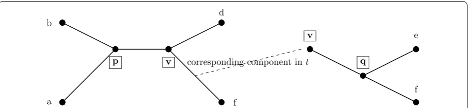
Before proceeding, we define the induced tree topol-ogy, tA, on a tree t and a subset of leaves A as follows.
Consider the minimal subtree of t that contains the leaves
A, and then suppress all nodes of degree two (i.e., replace all maximal paths of degree two nodes by a single edge). The endpoints of an edge e∈tA correspond to vertices in t and so e corresponds to a (possibly length 1) path in t; we denote the corresponding endpoints of e as et(u) and
et(v). For an induced tree tA, the component in t corre-sponding to an edge e∈tA is the set of edges and
verti-ces that can be reached by a walk starting from et(u) and ending at et(v) without using et(u) or et(v) multiple times. Note this will be a subgraph of t that includes et(u) and
et(v) as leaves. See Fig. 4.
When working with constraint trees, we alter the inser-tion algorithm to account for the constraints. Recall that the constraint trees are on disjoint sets of taxa. Thus, when inserting a taxon, we identify the corresponding constraint tree tc that includes that new taxon. Let A
be the set of taxa shared between tc and t and note that
tcA=tA since the trees are consistent. Thus, in tcA∪{x}, the taxon x can be viewed as being attached to some edge e
in tA. The eligible edges are in the component in t cor-responding to e. We then simply run INC on the compo-nent to find the desired edge of insertion.
INC−NJ
We continue by presenting the O(n2)INC−NJ method,
which is AFC and uses neighbor joining on carefully selected subsets to achieve this running time. Given the selected threshold q, we take our threshold graph
TG(d, q) and compute a greedy disjoint clique decompo-sition, such that each clique is of size O(√n). This is done by a simple ball-growing procedure that is interrupted when the ball includes more than O(√n) vertices; it is easy to see this takes O(n2) time. Next, we run NJ on each
a
b d
f
v
p corresponding component int
v
q
e
f
of these clique; this produces a set of neighbor joining subset trees that will serve as our constraint trees. Since the subsets are disjoint, the subset trees are guaranteed to be compatible (meaning that a compatibility supertree exists). Finally, if ǫ(q) <f/2, then the following theorem guarantees that all constraint trees produced by our tech-nique are correct. Furthermore, since NJ applied to each
clique of size O(√n) takes at most O(n1.5) time, our total runtime over all cliques is O(n2).
Theorem 7 Neighbor Joining (NJ) will recover the true tree T whenever the input matrix d satisfies
L∞(d,D) <f/2,whereDis an additive matrix defining
an edge-weighted version of the true tree T and f is the shortest internal branch weight in T. Furthermore, the runtime and space complexity isO(n3).
Proof The first sentence follows from [4]. The second sen-tence follows easily from the description of the algorithm.
Theorem 8 INC−NJis AFC and has runtime and space complexityO(n2)(assuming distances are precomputed).
Proof Follows directly from combining Theorems 6 and
7.
Boosting INC using other constraint trees
The version of constrained-INC we presented in the previous section achieves an optimal running time, but is based on obtaining constraint trees using neighbor joining on small subsets. However, we could modify the decomposition to produce larger subsets and thus take advantage of the likely improvement in accuracy obtained by using neighbor joining on these larger sub-sets to produce the constraint trees. This would still pro-duce a polynomial time algorithm, but one with a higher (and hence suboptimal) running time.
Another variation would be to use other phylogeny estima-tion methods besides neighbor joining. In particular, maxi-mum likelihood could be used to construct the constraint trees. As shown in [3], maximum likelihood under the CFN model is AFC. Hence, running maximum likelihood on sub-sets of the taxon set produced using the same technique as for INC−NJ will provide correct subset trees from
polyno-mial length sequences with high probability. Hence, the same approach we describe for use with neighbor joining (where that subset trees are computed using neighbor joining) can be modified to be used with maximum likelihood, and will be an AFC method. One negative impact of doing this would be running time, since maximum likelihood is NP-hard [24] and heuristics for maximum likelihood are computationally more intensive than neighbor joining.
Extension to the generalized time reversible (GTR) Markov models
In this section, we extend our AFC convergence guar-antees to the generalized time reversible (GTR) Markov model [20], which is the most commonly used site evolu-tion model used in phylogenetics. We will show that INC is AFC for the GTR model, drawing on established tech-niques and theory which we now present and summarize. The GTR model can be seen as a special case of the general Markov model [25], which we first describe. Under the general Markov model on m≥2 states, we have a rooted binary tree T with some distribution of states π >0 at the root of the tree and m-by-m
stochas-tic transition matrices M(e) for each edge e of T. Starting with a random sequence drawn i.i.d. from π, each site of the sequence evolves i.i.d. down the tree, according to the transition matrices specified by the model.
Definition 6 (GTR model) Let be the set of states with || =m. Let Q be an m×m rate matrix with Qij>0 for i�=j and
j∈Qij =0 for all i∈. Assume
that Q satisfies detailed balance with respect to π, or
πiQij=πjQji. Then, the General Time Reversible model is a general Markov model on with π as the initial state
distribution and M(e)=eτeQ for some τ
e>0 for each edge.
Note that the GTR model captures the CFN model by setting m=2,π =(1/2, 1/2) and
If we just consider one site, let fij(α,β) be the
probabil-ity that leaf i is in state α and leaf j is in state β. By some indexing of the states, we can form a m-by-m square matrix Fij= [fi,j(α,β)]. Then, we define the true distance function to be Dij= −log det(Fij). Let fˆij(α,β) be the
empirical probability (or relative frequency) that leaf i
and leaf j are in state α,β respectively, calculated by
tak-ing a simple average over all k sequence sites. Similarly, we define Fˆij = [ˆfi,j(α,β)] and the empirical distance function to be dij = −log det(Fˆij). This log-det distance function is well-known for the general Markov model (and hence applicable for its submodels, including the GTR model) and is a generalization of the CFN distance function that also satisfies similar properties [25]. Note that the empirical distance function will converge to the true distance function as the number of sites k→ ∞. With this extended definition of dij,Dij, we define ǫ(q)
similarly.
Note that det(M(e)) takes the values 1 or – 1 precisely if M(e) is a permutation matrix. Also, for the CFN model,
det(M(e))=1−2p(e), where p(e) is the substitution Q=
−1/2 1/2 1/2 −1/2
probability on edge e; thus we know that det(M(e)) >0 and det(M(e))→0 as p(e)→0.5, which correctly
sup-ports the intuition that information loss is large when
p(e) is close to 0.5. In general, (1/2)[1−det(M(e))] plays
the role of p(e) in the general model and −log(det(M(e))) is the corresponding w(e).
Thus, the natural extension of CFNf,g model to the GTR
model, GTRf,g, is to enforce f ≤ −log(det(M(e)))≤g for all edges in all model trees in GMf,g.
Definition 7 A phylogeny estimation method is said to be absolute fast converging (AFC) under the GTR model if, for all positive values f,g,ǫ (with f ≤g ), there
is a polynomial p such that for all GTR model trees T in
GTRf,g, the method will recover T given sequences of length k=O(p(n)) with probability at least 1−ǫ.
Now, we apply INC with the extended version of the empirical distance matrix and we define TG(d, q), q0,
ǫ(q) analogously for our generalized distance measure.
Note that by our Markov property and time-reversi-bility, if P is the unique path between leaves i, j in T, then the true distance matrix is additive and satisfies Dij=e∈P−log(det(M(e))) up to a constant shift [8]. Thus, if ǫ(q) <f/2, then applying a quartet query via the Four Point Method will return the accurate quartet tree. Therefore, the claim that INC is AFC for the GTR model follows immediately after we establish a slightly extended concentration bound.
Theorem 9 For k=�(ln(nf/ǫ)2 e4q), with probability
≥1−ǫ,we haveǫ(q) <f/2for allq=O(glogn)in the
GTR model.Furthermore, ifq0is the minimum value ofq such thatTG(d, q)is connected, thenq0=O(glogn)and
q0≥f/2.
Proof Since the log-det distance function is still addi-tive and corresponds to a tree metric with f, g still as minimum and maximum distances of an edge in the tree metric, our proof for the GTR model follows analogously once the following concentration equality is proved:
By Hadamard’s inequality, we note that
Since m is regarded as a constant (for DNA models, m=4 ) and since Fij,Fˆij are matrices whose entries
P(|det(Fˆij)−det(Fij)| ≥x)≤e−�(kx
2)
det(Fijˆ )−det(Fij)
≤mm+1
Fˆij−Fij
maxmax
Fij
max,
Fˆij
max
denote frequencies or probabilities and thus are all bounded by 1, we conclude that it suffices to prove:
For each of the m2 entries of Fˆij,Fij, which are
ˆ
fij(α,β),fij(α,β) respectively for all pairs of states
α,β∈�, we can prove concentration by applying
Azu-ma’s inequality (Theorem 4) for sum of k indicators.
And our conclusion follows.
Theorem 10 INCis absolute fast converging for the GTR model and takes O(n2) time and space (assuming
dis-tances are precomputed).
Discussion
This paper presents a novel algorithmic technique for constructing phylogenetic trees, which allows statisti-cally consistent and highly accurate methods to be used on subsets of the taxa in a divide-and-conquer frame-work. We proved that several of these variants are abso-lute fast converging (AFC) under the CFN and GTR sequence evolution models, and that some of these meth-ods achieve O(n2) time and space (where n is the num-ber of sequences) once the dissimilarity matrix relating the sequences is computed. More generally, tree estima-tion methods could be scaled to large datasets using this approach, provided that it is possible to compute a matrix of pairwise distances that is guaranteed to converge to an additive matrix as the amount of data increases.
Many of the ideas in the algorithmic design of INC are derived from prior algorithms for similar problems. For example, the node query insertion procedure was explored earlier in [26, 27] to produce a fast O(nlogn) tree-growing algorithm, but analyzed under a different model of quartet tree error than we use here; further-more, a direct implementation of their model does not produce an AFC algorithm. The idea of using a distance matrix to combine disjoint trees was originally presented in [28] in the context of multi-locus species tree estima-tion; that technique (called NJMerge) is a modification of the neighbor joining method [18] to allow for constraint trees. Since neighbor joining is not AFC [29], it seems unlikely that NJMerge can be used to produce an AFC method.
The goal of this work was improved empirical per-formance, compared to prior AFC methods. One of the interesting aspects of INC is the potential to use it with disjoint constraint trees. As noted in this paper,
P Fˆij−Fij
max≥x
≤e−�(kx2)
P
fˆij(α,β)−fij(α,β) ≥x
maximum likelihood (if solved exactly) is AFC under the standard sequence evolution models, and although it is NP-hard to solve exactly there are many seemingly good heuristics for maximum likelihood (e.g., RAxML [30]). One possible technique that could result in excel-lent empirical accuracy and scalability is to use a maxi-mum likelihood heuristic to compute constraint trees, and then combine the constraint trees using constrained INC. The value of such an approach, however, depends on the decomposition strategy, as not all decomposi-tions will produce AFC methods. Consider, for example, the impact of selecting quartets from a large phylogeny: if these quartets are selected arbitrarily, it is possible to produce quartets whose true trees fall in the Felsenstein Zone, where methods such as maximum parsimony are not statistically consistent and maximum likelihood— although consistent—will tend to have poor accuracy unless very long sequences are available [31, 32]. There-fore, the use of constrained INC with maximum likeli-hood, or any other tree estimation method, will only be AFC for some decomposition strategies (and not for arbi-trary ones), and may not provide accuracy advantages except when combined with carefully designed decom-position strategies.
Thus, additional work is needed to develop provably AFC divide-and-conquer strategies that enable this kind of approach to be used to the greatest empirical advan-tage on large challenging phylogenetic datasets.
Authors’ contributions
Established theory: QZ, SR, TW. Made figures: QZ. Wrote paper: QZ, SR, TW. All authors read and approved the final manuscript.
Author details
1 Department of Mathematics, University of California Berkeley, Evans Hall, Berkeley, CA 94720, USA. 2 Department of Computer Science, University of California Berkeley, SODA Hall, Berkeley, CA 94720, USA. 3 Department of Computer Science, University of Illinois Urbana-Champaign, 201 N. Good-win Avenue, Urbana, IL 61801, USA.
Acknowledgements
The authors thank Mike Steel for helpful discussions, and the reviewers whose suggestions led to improvements in the manuscript.
Competing interests
The authors declare that they have no competing interests. Ethics approval and consent to participate
Not applicable. Funding
Supported by U.S. National Science Foundation Grant 1535989 (to SR) and 1535977 (to TW).
Publisher’s Note
Springer Nature remains neutral with regard to jurisdictional claims in pub-lished maps and institutional affiliations.
Received: 27 September 2018 Accepted: 18 January 2019
References
1. Neyman J. Molecular studies of evolution: a source of novel statistical problems. Statistical decision theory and related topics. New York: Aca-demic Press; 1971. p. 1–27.
2. Cavender JA. Taxonomy with confidence. Math Biosci. 1978;40(3–4):271–80.
3. Roch S, Sly A. Phase transition in the sample complexity of likelihood-based phylogeny inference. Probab Theory Relat Fields. 2017;169(1):3–62. 4. Atteson K. The performance of neighbor-joining methods of
phyloge-netic reconstruction. Algorithmica. 1999;25(2–3):251–78.
5. Warnow T. Computational phylogenetics: an introduction to designing methods for phylogeny estimation. Cambridge: Cambridge University Press; 2018.
6. Quast C, Pruesse E, Yilmaz P, Gerken J, Schweer T, Yarza P, Peplies J, Glöck-ner FO. The SILVA ribosomal RNA gene database project: improved data processing and web-based tools. Nucleic Acids Res. 2012;41(D1):590–6. 7. Erdös P, Steel MA, Székely L, Warnow T. A few logs suffice to build (almost)
all trees (i). Random Struct Algorithms. 1999;14:153–84.
8. Erdös P, Steel MA, Székely L, Warnow T. A few logs suffice to build (almost) all trees (ii). Theor Comput Sci. 1999;221:77–118.
9. Warnow T, Moret BME, St. John K. Absolute convergence: true trees from short sequences. In: Proceedings of SODA. Society for Industrial and Applied Mathematics; 2001. p. 186–95.
10. Nakhleh L, Roshan U, St. John K, Sun J, Warnow T. Designing fast converg-ing phylogenetic methods. Bioinformatics. 2001;17(suppl–1):190–8. 11. Roch S. Sequence-length requirement for distance-based phylogeny
reconstruction: breaking the polynomial barrier. In: Proceedings of the IEEE Symposium on Foundations of Computer Science (FOCS); 2008. p. 729–38.
12. Roch S. Towards extracting all phylogenetic information from matrices of evolutionary distances. Science. 2010;327(5971):1376–9.
13. Mihaescu R, Hill C, Rao S. Fast phylogeny reconstruction through learning of ancestral sequences. Algorithmica. 2013;66(2):419–49.
14. Brown DG, Truszkowski J. Fast phylogenetic tree reconstruction using locality-sensitive hashing. In: Workshop on algorithms for bioinformatics (WABI). Springer, New York; 2012. p. 14–29.
15. Mossel E. Phase transitions in phylogeny. Trans Am Math Soc. 2004;356(6):2379–404.
16. Csűrös M. Fast recovery of evolutionary trees with thousands of nodes. J Comput Biol. 2002;9(2):277–97.
17. King V, Zhang L, Zhou Y. On the complexity of distance-based evolu-tionary tree reconstruction. In: 14th annual ACM-SIAM symposium on discrete algorithms (SODA). Society for Industrial and Applied Mathemat-ics; 2003. p. 444–53.
18. Saitou N, Nei M. The neighbor-joining method: a new method for recon-structing phylogenetic trees. Mol Biol Evol. 1987;4(4):406–25.
19. Warnow T. Supertree construction: opportunities and challenges. 2018. arXiv :1805.03530 [q-bio.PE]
20. Tavaré S. Some probabilistic and statistical problems in the analysis of DNA sequences. Lectures on mathematics in the life sciences, vol. 17. Providence: American Mathematical Society; 1986. p. 57–86. 21. Huson D, Nettles S, Parida L, Warnow T, Yooseph S. The disk-covering
method for tree reconstruction. In: Algorithms and experiments (ALEX). 1998. p. 62–75.
22. Buneman P. A note on the metric properties of trees. J Comb Theory (B). 1974;17:48–50.
23. Azuma K. Weighted sums of certain dependent random variables. Tohoku Math J Second Ser. 1967;19(3):357–67.
24. Roch S. A short proof that phylogenetic tree reconstruction by maximum likelihood is hard. IEEE/ACM Trans Comput Biol Bioinform. 2006;3(1):92–4. 25. Steel MA. Recovering a tree from the leaf colourations it generates under
a Markov model. Appl Math Lett. 1994;7(2):19–23.
26. Brown DG, Truszkowski J. Fast error-tolerant quartet phylogeny algo-rithms. In: Annual symposium on combinatorial pattern matching. Springer, New York; 2011. p. 147–61.
27. Truszkowski J, Hao Y, Brown DG. Towards a practical O(n log n) phylogeny algorithm. Algorithms Mol Biol. 2012;7(1):32.
•fast, convenient online submission •
thorough peer review by experienced researchers in your field • rapid publication on acceptance
• support for research data, including large and complex data types •
gold Open Access which fosters wider collaboration and increased citations maximum visibility for your research: over 100M website views per year •
At BMC, research is always in progress.
Learn more biomedcentral.com/submissions
Ready to submit your research? Choose BMC and benefit from: 29. Lacey MR, Chang JT. A signal-to-noise analysis of phylogeny estimation
by neighbor-joining: insufficiency of polynomial length sequences. Math Biosci. 2006;199(2):188–215. https ://doi.org/10.1016/j.mbs.2005.11.003. 30. Stamatakis A. RAxML version 8: a tool for phylogenetic analysis and
post-analysis of large phylogenies. Bioinformatics. 2014;30(9):1312–3.
31. Felsenstein J. Cases in which parsimony or compatibility methods will be positively misleading. Syst Zool. 1978;27(4):401–10.