Remote sensing of sea ice: advances during the DAMOCLES project

The Cryosphere, 6, 1411–1434, 2012 www.the-cryosphere.net/6/1411/2012/ doi:10.5194/tc-6-1411-2012

© Author(s) 2012. CC Attribution 3.0 License.

The Cryosphere

Remote sensing of sea ice: advances during the DAMOCLES project

G. Heygster1, V. Alexandrov2, G. Dybkjær4, W. von Hoyningen-Huene1, F. Girard-Ardhuin3, I. L. Katsev5, A. Kokhanovsky1, T. Lavergne6, A. V. Malinka5, C. Melsheimer1, L. Toudal Pedersen4, A. S. Prikhach5, R. Saldo7, R. Tonboe4, H. Wiebe1, and E. P. Zege5

1_{Institute of Environmental Physics, University of Bremen (UB), Germany}

2_{Nansen International Environmental and Remote Sensing Centre (NIERSC), St. Petersburg, Russia and Nansen} Environmental and Remote Sensing Centre, Bergen, Norway

3_{Institut Franc¸ais de Recherche pour l’Exploitation de la Mer (IFREMER) , Plouzan´e, France} 4_{Danish Meteorological Institute (DMI), Denmark}

5_{B.I. Stepanov Institute of Physics of the National Academy of Sciences of Belarus (IP-NASB), Minsk, Belarusian} 6_{Norwegian Meteorological Institute (met.no), Oslo, Norway}

7_{Danish National Space Center (DNSC), Copenhagen, Denmark}

Correspondence to: G. Heygster ([email protected])

Received: 29 November 2011 – Published in The Cryosphere Discuss.: 3 January 2012 Revised: 22 August 2012 – Accepted: 13 October 2012 – Published: 3 December 2012

Abstract. In the Arctic, global warming is particularly pro-nounced so that we need to monitor its development contin-uously. On the other hand, the vast and hostile conditions make in situ observation difficult, so that available satellite observations should be exploited in the best possible way to extract geophysical information. Here, we give a r´esum´e of the sea ice remote sensing efforts of the European Union’s (EU) project DAMOCLES (Developing Arctic Modeling and Observing Capabilities for Long-term Environmental Stud-ies). In order to better understand the seasonal variation of the microwave emission of sea ice observed from space, the monthly variations of the microwave emissivity of first-year and multi-year sea ice have been derived for the frequen-cies of the microwave imagers like AMSR-E (Advanced Mi-crowave Scanning Radiometer on EOS) and sounding fre-quencies of AMSU (Advanced Microwave Sounding Unit), and have been used to develop an optimal estimation method to retrieve sea ice and atmospheric parameters simultane-ously. In addition, a sea ice microwave emissivity model has been used together with a thermodynamic model to establish relations between the emissivities from 6 GHz to 50 GHz. At the latter frequency, the emissivity is needed for assimilation into atmospheric circulation models, but is more difficult to observe directly. The size of the snow grains on top of the sea ice influences both its albedo and the microwave emission. A method to determine the effective size of the snow grains

1 Introduction

Sea ice is an essential component of the climate system at high latitudes. It influences weather and climate on both re-gional and global scales. Sea ice is an efficient insulator that strongly reduces fluxes of heat and vapour between ocean and atmosphere, where even a few percent of open water or refrozen thin ice in the Arctic sea ice may increase the heat flux between ocean and atmosphere drastically and increase 2 m air temperatures by several degrees (L¨upkes et al., 2008). The combination of thinning Arctic sea ice and the positive albedo feedback mechanism, caused by relative low albedo of the open ocean, are considered the main reasons for the signal of global warming to be amplified in the Arctic (Ser-reze et al., 2009). Sea ice extent, concentration, drift and de-formation are therefore important parameters for both cou-pled climate circulation models and for operational applica-tions like numerical weather prediction. These characteristics must be monitored continuously. The goal of this review is to combine and bundle the progress of sea ice remote sensing capabilities achieved during the project DAMOCLES (De-veloping Arctic Modeling and Observing Capabilities for Long-term Environmental Studies) conducted from 2006 to 2010. DAMOCLES was one of the main European contribu-tions to the International Polar Year.

For observing sea ice from space, passive microwave sen-sors have the advantages of not requiring sunlight (they ob-serve thermal radiation) and can thus also collect measure-ments during the (polar) night, and are also widely inde-pendent of cloud cover. Moreover, their availability since 1972 makes passive microwave observations the longest of all satellite records available and allows for analyses on cli-mate time scales. However, the amount of emitted radiation (radiance) is much higher and varies much more over sea ice than over open water, making it difficult to estimate areas covered by the main sea ice type (first-year ice or multi-year ice) and to determine atmospheric quantities from microwave observations over sea ice. The necessary step to improve this situation of better estimating the microwave emissivity at the microwave observing frequencies is presented in Sect. 2.1, together with an application to retrieve both surface and at-mospheric parameters over sea ice. As an attempt to pre-dict the sea ice emissivity from the meteorological history, Sect. 2.3 combines a sea ice emissivity model with a ther-modynamic model, driven with ECMWF atmospheric model data (Tonboe, 2010).

Knowledge of the sea ice temperature is required to deter-mine the energy flux between ocean and atmosphere. It is rel-evant when retrieving the microwave emissivity (see above), and is needed to determine the atmospheric temperature pro-file from data of temperature sounders like AMSU-A (part of AMSU). In thermodynamic equilibrium, the vertical temper-ature profile within the sea ice and snow pack is characterized by the snow surface temperature and the snow/ice interface temperature. Section 3 investigates the relation between these

two quantities and the brightness temperatures, together with a study investigating which microwave frequencies are best suited as proxies for assimilation in atmospheric circulation models.

Snow on top of the sea ice is relatively slight in mass, but crucial for climate change studies because not only the area covered by snow and ice is reduced with time (Seidel and Martinec, 2004), but also the snow strongly influences the albedo of the sea ice, and thus the local radiative balance that plays an essential role for the albedo feedback process. The albedo of snow does not have a constant value, but depends on the grain size (with smaller grains having higher albedo) and the amount of pollution like soot (e.g. in Eurasia, Hansen and Nazarenko, 2004) and in fewer cases dust, which both lower the albedo significantly. Other factors contributing to snow and sea ice albedo are the solar zenith angle, cloud cover, surface tilt and even air humidity (Pirazzini, 2004). DAMOCLES has contributed to our remote sensing capabil-ities for the snow grain size (Sect. 4.1), which is based on the knowledge of the reflectance function (Sect. 4.2), and to the retrieval of the albedo itself (Sect. 4.3).

Sea ice drift and deformation are dynamic parameters in-fluencing the open water fraction and ice thickness distribu-tion and hence the energy and mass balance of the Arctic sea ice. Section 5 presents progress, in the detection of sea ice drift and deformation derived from the METOP instru-ments scatterometer ASCAT, the optical radiometer AVHRR, from ASCAT (Advanced Synthetic Aperture Radar) on EN-VISAT and from passive microwave radiometers on Aqua and DMSP satellites.

Information on sea ice thickness is needed to determine the ice volume, to compute the ice mass exchanges with the ocean, to validate numerical models of the ocean circula-tion as well as to plan ship and offshore operacircula-tions in the ice. In the last 10 yr, radar altimeter data from ERS and EN-VISAT have been used to determine the inter-annual changes in sea ice thickness through direct measurements of sea ice freeboard. The contribution of DAMOCLES, presented in Sect. 6, was an investigation on the relation between free-board and ice thickness based on the airborne Sever expedi-tions conducted between 1928 and 1993.

2 Sea ice microwave emissivity

2.1 Emissivity determination

The satellite observed radiance, called brightness tempera-tureTb=Tem×ε, is the product of the physical temperature

Tem of the isothermal emitting layer and the emissivityε, a material parameter. Over open ocean, microwave observa-tions have been used for many decades to determine a wide range of surface and atmospheric parameters such as surface temperature, wind speed, atmospheric total water vapour, liq-uid water and precipitation. Over sea ice, we so far only have

G. Heygster: Remote sensing of sea ice: progress from DAMOCLES project 1413

been able to retrieve concentrations (percentage of surface cover) of total ice (Andersen et al., 2007) and multi-year ice (ice having survived at least one summer melt season) (Cava-lieri et al., 1984; now used with tie points from Comiso et al., 1997). The reason why we can extract so much less geophys-ical information from microwave observations over sea ice is the high and highly varying sea ice emissivity, making it dif-ficult to determine the much smaller atmospheric component of the received radiation. In the frequency range from 6 to 90 GHz, the emissivity of open water increases from about 0.4 to 0.6 (with the vertically polarized emissivity about 0.25 higher than the horizontal one), whereas that of first-year ice varies between 0.85 and 0.95, and that of multi-year ice be-tween 0.9 and 0.55 (Spreen et al., 2008). However, the uncer-tainty in the emissivity of open water, influenced by temper-ature and wind speed, increases in the same frequency range from 0.2 to 2.1 K (Wentz, 1983), but that of sea ice varies according to ice type and frequency between 6 K (first-year ice at 6 GHz) and 16 K (multi-year ice at 37 GHz) (Eppler et al., 1992). Moreover, the microwave radiation emanates, compared to water, from much deeper layers of snow and ice where the meteorological history is frozen in the micro-physical parameters, resulting in a much more complex re-lationship between physical properties of the snow/ice com-plex and the microwave radiances. As a consequence, reli-able emissivity forward models, while existing for open wa-ter (e.g. Wentz, 1983), remain a challenge for the case of sea ice (Tonboe et al., 2006).

As an additional difficulty, in winter the high vertical tem-perature gradient within the sea ice from about−30◦C at the surface to−1.8◦_{C at the bottom complicates the} deter-mination of the temperature of the emitting layer at the dif-ferent observing frequencies, which span the range from 6 to 183 GHz and have different penetration depths. In order to characterize the temperature of an emitting layer that is not isothermal, but has a temperature gradient by a single scalar instead by a temperature profile, the concept of effective tem-perature is used. It is the temtem-perature of a layer identical to the emitting layer, except being of homogeneous tempera-ture, and emitting the same radiation as the layer with the temperature profile. This concept will be used in the next sec-tion on emissivity modelling.

Within DAMOCLES, the annual cycle of the emissivities of first-year and multi-year sea ice, the two most promi-nent ice types, were determined at all microwave observ-ing frequencies of the sensors Advanced Microwave Sound-ing Unit (AMSU, consistSound-ing of the temperature soundSound-ing part AMSU-A at lower frequencies and the humidity sound-ing part AMSU-B at higher frequencies) for the year 2005 (Matthew et al., 2008) and Advanced Microwave Scanning Radiometer on EOS (AMSR-E) (Matthew et al., 2009). The horizontal resolutions of AMSU-A and B are 48 km and 16 km at nadir, where each 3 observations of AMSU-B are combined to correspond to one AMSU-A footprint. The

res-olution of AMSR-E varies with frequency (6.9...89 GHz) be-tween 43×75 km and 3.5×5.9 km.

In both studies, the emissivity is retrieved over two Arc-tic regions, one covered by first-year ice (76.5–78◦N, 77– 79◦E) in the Kara Sea and one covered by multi-year ice (84–85.5◦N, 31.5–36◦W) north of Greenland. Knowledge about the surface temperature and atmospheric temperature and humidity profiles is provided from ECMWF ERA-40 re-analysis data available every 6 h in a grid of about 120 km resolution and with 60 vertical levels. Vertical temperature profile within the snow and sea ice pack are taken from the Heat Budget of the Arctic Ocean (SHEBA) observations in 1997 and 1998 (Ulbay et al., 2002) and penetration depth data from Haggerty and Curry (2001) are used to estimate the temperature of the emitting layer, using a linear regression. The discrepancy in time and space between satellite and in situ observations may introduce an error in the analysis, es-pecially in view of a climatological change, but this was the best combination of data available at the time of the study. The emissivityε(ν,θ) at frequencyνand incidence angleϑ

is retrieved as the ratio(Tb(ν, θ )−Tb,0)/(Tb,1−Tb,0) where

Tb(ν, θ) is the observed brightness temperature, andTb,0and

Tb,1are simulated brightness temperatures determined from known atmospheric profiles (Matthew et al., 2009).

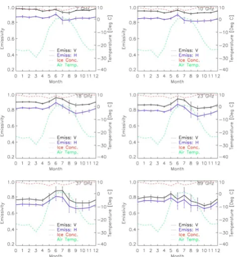
Here we present as examples the monthly averaged re-sults for first-year ice (Fig. 1) and multi-year ice (Fig. 2) for the AMSR-E frequencies ranging from 7 to 89 GHz. During the winter months, the surface emissivity and the concentra-tions of first-year ice shown also in Fig. 1 are near unity and the difference between horizontally and vertically polarized emissivity is low. During the months of June, July, and Oc-tober, the satellite footprints may contain both ice and open water, leading to high variability (error bars) of the deter-mined average emissivity. During August and September, the ice has completely melted and the emissivity of open water is observed. The monthly variation of multi-year ice (Fig. 2) remains nearly constant for all months except the summer months from May to September when the higher emissiv-ity values are observed, with a maximum of 0.95 at 7 GHz in June. The retrieved emissivities agree well with those of AMSU in the sense that for similar frequencies similar emis-sivities are found. As the polarization of the AMSU measure-ments varies with incidence angle, for such a comparison first the polarizations of the AMSR-E observations (horizontal and vertical) need to be converted to those of the AMSU ob-servations at the AMSR-E incidence angle of 50◦_(Matthew et al., 2009). For the first time, also the correlations between the emissivities at different frequencies and polarizations of AMSR-E have been determined (Mathew et al., 2009). The covariances, which are easily derived from the correlations, are required when assimilating the brightness temperatures into atmospheric and ocean circulation models.

operational processing chain of the Norwegian Meteorolgo-ical Institute (Schyberg and Tveter, 2009, 2010).

Another important application of the emissivities is the re-trieval of atmospheric parameters over sea ice, similarly as has been done over open ocean from passive microwave sen-sors for more than three decades. The idea is to model the ra-diances of the AMSR-E channels with a forward model that takes surface and atmospheric parameters as input, and then use an inverse method to retrieve these parameters (state ables) from the measured AMSR-E radiances. The state vari-ables here are surface wind speed, total column water vapour (TWV), cloud liquid water path (CLW), sea surface tempera-ture, ice surface effective temperatempera-ture, sea ice concentration, and multi-year ice fraction. Note that the ice surface temper-ature is in fact the effective tempertemper-ature of the emitting layer of the snow/ice complex, as introduced and described in the previous section.

The forward model is based on the one by Wentz and Meissner (2000) that simulates AMSR-E radiances over open water given wind speed, TWV, CLW, and surface tempera-ture. We have modified this forward model to allow partial or full ice cover of the sea. This in turn requires knowledge of the sea ice emissivity of first-year ice and multi-year ice which is taken from the method mentioned above.

The inverse method, the “optimal estimation method” (Rodgers, 2000), requires a priori data and covariances for all state variables. The a priori data for the ice concentration are directly determined from the AMSR-E brightness tem-peratures (using the NASA Team algorithm), and the a priori surface temperatures are derived from the AMSR-E bright-ness temperatures, the ice concentration and the sea ice emis-sivities using the iterative method of the bootstrap algorithm as described by Comiso et al. (2003). The remaining a priori data are taken from meteorological analysis data (ECMWF). The solution has to be found by an iteration scheme (New-ton method), and comprises not just the retrieved state vari-ables, but also includes the a posteriori covariance matrix that contains the standard deviations (the uncertainties) of the re-trieved variables and their mutual correlations.

The retrieval produces fields (swath by swath) of the state variables. The entire Arctic can be covered daily. However, mainly in areas of multi-year ice, the retrieval shows slow convergence – the most probable reason being that the emis-sivities of multi-year ice are not well enough represented in the forward model, as they are based on emissivity val-ues retrieved for a certain area (85–85.5◦_{N, 31.5–36}◦_{W, see} above).

2.2 Emissivity modelling; combination with thermodynamic model

It has been demonstrated that the seasonal variability of ther-mal microwave emission can be simulated using a combi-nation of thermodynamic model and emission modelling. Combined thermodynamic and emissivity models generate

long snow/sea ice/microwave time series that can be used for statistical analysis of radiometer sea ice data sensitivi-ties (M¨atzler et al., 2006). The purpose is not necessarily to reproduce a particular situation in time and space but rather to provide a realistic characterisation of the daily to seasonal variability.

In DAMOCLES the microwave emission processes from sea ice have been simulated using the combination of a one dimensional thermodynamic sea ice model and a microwave emission model (Tonboe, 2010; Tonboe et al., 2011). The emission model is the sea ice version of the Microwave Emis-sion Model for Layered Snow-packs (MEMLS) (Wiesmann and M¨atzler, 1999; M¨atzler et al., 2006) It uses the theoret-ical improved Born approximation for estimating scattering, which validates for a wider range of frequencies and scatterer sizes than the empirical formulations (M¨atzler and Wies-mann, 1999). Using the improved Born approximation, the shape of the scatters is important for the scattering magnitude (M¨atzler, 1998). We assume spherical scatters in snow when the correlation length, a measure of grain size, is less than 0.2 mm and the scatters are formed as cups when greater than 0.2 mm to resemble depth hoar crystals. The sea ice version of MEMLS includes models for the sea ice dielectric prop-erties while using the same principles for radiative transfer as the snow model. Again the scattering within sea ice lay-ers beneath the snow is estimated using the improved Born approximation. The scattering in multi-year ice is assumed from small air bubbles within the ice. The emission model is used to simulate the sea ice Tb’s and emissivity where the subscript v or h and number denote the polarization at oblique incidence angles and the frequency in GHz, respec-tively, e.g.ev89for the emissivity at 89 GHz and vertical po-larization. All simulations are at 50◦_{incidence angle similar} to SSMIS and other conically scanning radiometers.

The thermodynamic model has the following prognostic parameters for each layer: thermometric temperature, den-sity, thickness, snow grain size and type, ice salinity and snow liquid water content. Snow layering is very important for the microwave signatures; therefore, it treats snow lay-ers related to individual snow precipitation events. For sea ice it has a growth rate dependent salinity profile. The sea ice salinity is a function of growth rate and water salinity (32 psu) (Nagawo and Sinha, 1981).

Climatology indicates that there is snow on multi-year ice at the end of summer melt in September (Warren et al., 1999). Therefore, the multi-year ice simulations are initiated on 1 September with an isothermal 2.5 m ice floe with 5-cm-old snow layer on top. The multi-year ice gradually grows at the six positions from 2.5 m to between 3.0 and 3.4 m in spring and snow depths during winter ranging between 0.2 and 0.5 m. The mean snow depth in this data set is 0.26 m and the mean ice thickness is 2.8 m. The snow/ice inter-face temperature is near 270 K in September and May and down to 230 K in March. The simulations are confined to these relatively cold conditions. The melt processes during

G. Heygster: Remote sensing of sea ice: progress from DAMOCLES project 1415

1 2 3 4 5 6 7

8

9

Figure 1. Seasonal variation of emissivities of first-year ice at AMSR-E frequencies,

(black) vertical and (blue) horizontal polarizations. (Top left) 7 GHz, 10 GHz, 18 GHz, 23 GHz, 37 GHz, and (bottom right) 89 GHz. Red dashed line: Ice concentration. Green dashed line: Air temperature. Months 0 and 12 are the same. From Matthew et al. (2009).

37

Fig. 1. Seasonal variation of emissivities of first-year ice at

AMSR-E frequencies, (black) vertical and (blue) horizontal polarizations. (Top left) 7, 10, 18, 23, 37 and (bottom right) 89 GHz. Red dashed line: ice concentration; green dashed line: air temperature. Months 0 and 12 are the same from Matthew et al. (2009).

the summer season are complicated and not sufficiently de-scribed by the thermodynamic model. Summer melt is there-fore not included in this study. The thermodynamic model is further described in Tonboe (2010) and Tonboe et al. (2011). The thermodynamic model is fed with ECMWF ERA 40 data input at 6 h intervals. The parameters used as input to the thermodynamic model are the surface air pressure, the 2 m air temperature, the 10 m wind speed, the incoming short-wave solar radiation, the incoming long-wave radiation, the dew-point temperature and precipitation. In return the thermody-namic model produces detailed snow and ice profiles which are input to the emission model at each time-step. The input to the emission model is snow and ice density, snow grain size and scatter size in ice, temperature, salinity and snow type. The layer thickness in the snow-pack is determined at each precipitation event and the subsequent metamorphosis.

Emissivity at 18, 36 and 89 GHz, its temporal variabil-ity, the gradient ratio at 18 and 36 GHz (GR18/36=(T36v−

T18v)/(T36v+T18v)), and the polarisation ratio at 18 GHz (PR18=(T18v−T18h)/(T18v+T18h)) are comparable to typ-ical signatures derived from satellite measurements (Tonboe, 2010).

The correlation between each of the multi-year ice param-eters – brightness temperature (Tv), emissivity (ev) and effec-tive temperature (Teff, see explanation in Sect. 2.1) – at neigh-bouring frequencies 18, 36 and 50 GHz is high (r≥0.94).

1 2 3 4 5

Figure 2. Seasonal variation of emissivities of multiyear ice at AMSR-E frequencies [(black) vertical and (blue) horizontal polarizations]. (Top left) 7 GHz, 10 GHz, 18 GHz, 23 GHz, 37 GHz, and (bottom right) 89 GHz. Red dashed line: Ice concentration. Green dashed line: Air temperature. Months 0 and 12 are the same. From Mathew et al. (2009).

38

Fig. 2. Seasonal variation of emissivities of multi-year ice at

AMSR-E frequencies [(black) vertical and (blue) horizontal polar-izations]. (Top left) 7, 10, 18, 23, 37 and (bottom right) 89 GHz. Red dashed line: ice concentration; green dashed line: air temperature. Months 0 and 12 are the same from Mathew et al. (2009).

The correlation between each of the 18 and 36 GHz multi-year ice parametersev,TeffandTvis equally good for phys-ical temperatures near the melting point and low tempera-tures during winter. The melting season is not included and the correlations are referring to snow ice interface temper-atures less than about 270 K and above 240 K (Tonboe et al., 2011). These lower frequencies (18–50 GHz) penetrate into the multi-year ice, while the penetration of the 89 GHz reaches only to the snow ice interface. The high frequency channels at 150 and 183 GHz are penetrating only the snow surface and the correlation between these is also high (r=

0.99). However, the emissivity of multi-year ice at 89 GHz,

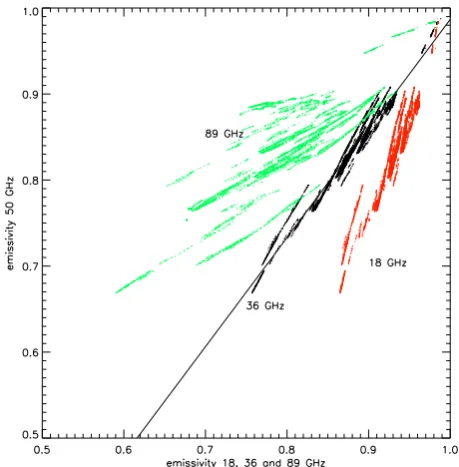
The emissivity is affected by volume scattering processes in the snow cover and also absorption in the upper ice. The GR18/36, which is a measurable proxy for scattering, is fur-ther related to the emissivity of multi-year iceev50at 50 GHz. The linear relationship between these two simulated param-eters seems to be robust over the wide range of temperatures and snow depths covered by the cases of Fig. 3. However, the relationships of Teff to measurable parameters such as air or surface temperature show less correlation because of the steep temperature gradient near the surface and the pen-etration depth variability. Nevertheless,Teff is highly corlated with that of neighbouring channels. The simucorlated re-lationship between GR18/36andev50suggests that it may be possible to estimate the microwave emissivity at the atmo-spheric sounding frequencies (∼50 GHz) from satellite mea-surements at lower frequencies seasonally across the Arc-tic Ocean with microwave instruments such as SSMIS, as it is done over open water. The emissivity of the sounding frequencies cannot be detected directly from observations in these channels because they are dominated by the atmo-spheric signal component, which in addition is difficult to separate from the surface contribution.

Test runs with the regional numerical weather prediction model HIRLAM (High Resolution Limited Area Model) where satellite microwave radiometer data from sea ice cov-ered regions were assimilated indicated that atmospheric temperature sounding of the troposphere over sea ice, which is not practiced in current numerical weather prediction mod-els, is feasible (Heygster et al., 2009). The test showed that the assimilation of AMSU-A near 50 GHz temperature sounding data over sea ice improved model skill on common variables such as surface temperature, wind and air pressure. These promising test results are the motivation for the new EUMETSAT Ocean and Sea Ice Satellite Application Facil-ity (OSI SAF) sea ice emissivFacil-ity model.

The OSISAF emissivity model is based on simulated cor-relations between the surface brightness temperature at 18 and 36 GHz and at 50 GHz. The model coefficients are tuned with simulated data from a combined thermodynamic and emission model in DAMOCLES. The intention with the model is to provide a first guess sea ice surface emissivity estimate for tropospheric temperature sounding in numeri-cal weather prediction models assimilating both AMSU and Special Sensor Microwave Imager/Sounder (SSMI/S) data (Tonboe and Schyberg, 2011).

3 Snow and sea ice temperatures

The snow surface temperature is among the most impor-tant variables in the surface energy balance equation and it strongly interacts with the atmospheric boundary layer struc-ture, the turbulent heat exchange and the ice growth rate.

The snow surface on thick multi-year sea ice in winter is on average colder than the air because of the negative radia-1

2 3 4 5

Figure 3. The simulated 18, 36 and 89 GHz emissivity at vertical polarisation of multiyear ice vs. the 50 GHz emissivity. The 18 GHz vs. the 50 GHz emissivity is shown in red, the 36 GHz vs. the 50GHz in black, and the 89 GHz vs. the 50GHz in green. The line is fitted to the 36 GHz vs. 50 GHz cluster: ev50=1.268ev36 - 0.28.

39

Fig. 3. The simulated 18, 36 and 89 GHz emissivity at vertical

polar-isation of multi-year ice vs. the 50 GHz emissivity. The 18 GHz vs. the 50 GHz emissivity is shown in red, the 36 GHz vs. the 50 GHz in black, and the 89 GHz vs. the 50 GHz in green. The line is fitted to the 36 GHz vs. 50 GHz cluster:ev50=1.268ev36−0.28.

tion balance (Maykut, 1986). Beneath the snow surface there is a strong temperature gradient with increasing temperatures towards the ice-water interface temperature at the freezing point around−1.8◦_{C. With the thermodynamic model} pre-sented in Tonboe (2010) and in Tonboe et al. (2011), the sea ice surface temperature and the thermal microwave bright-ness temperature were simulated using a combination of ther-modynamic and microwave emission models (Tonboe et al., 2011).

The simulations indicate that the physical snow/ice inter-face temperature or alternatively the 6 GHz effective tem-perature have a good correlation with the effective temper-ature at the tempertemper-ature sounding channels near 50 GHz. The physical snow/ice interface temperature is related to the brightness temperature at 6 GHz vertical polarisation as ex-pected. The simulations reveal that the 6 GHz brightness tem-perature can be related to the snow/ice interface temtem-perature correcting for the temperature dependent penetration depth in saline ice. The penetration is deeper at colder temperatures and shallower at warmer temperatures. This means the 6 GHz

Teffis relatively warmer than the snow/ice interface temper-ature at colder physical tempertemper-atures because of deeper pen-etration, in line with the findings of Ulaby et al. (1986) that the penetration depth increases with decreasing temperatures Nevertheless, it may be possible to derive the snow/ice in-terface temperature from the 6 GHz brightness temperature. The snow/ice interface temperature estimate may be more

G. Heygster: Remote sensing of sea ice: progress from DAMOCLES project 1417

0 10 20 30 40 50 60 70 80 90

0.0 0.4 0.8 1.2 1.6 2.0

Cs

(p

p

m

)

solar angle (degree) MIX

0 10 20 30 40 50 60 70 80 90

0 20 40 60 80 100 120 140 160 180 200

MIX

aef

(



m)

solar angle (degree)

1

2

3

Figure 4. Retrieval of effective snow grain size and soot concentration by two methods: SGSP (-x) and

LUT-Mie (-o).

Nadir observation. Horizontal lines mark true values.

40

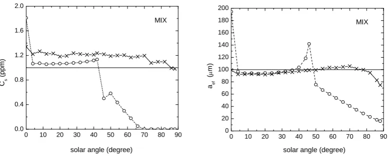
Fig. 4. Retrieval of effective snow grain size and soot concentration by two methods: SGSP (−×) and LUT-Mie(−); Nadir observation. Horizontal lines mark true values.

easily used in physical modelling than the effective tempera-ture. Hydrodynamic ocean and sea ice models with advanced sea ice modules simulate the snow surface and snow/ice tem-peratures explicitly.

The simulations with the combined thermodynamic and emission model show that the 6 GHz brightness or effec-tive temperature estimates (Hwang and Barber, 2008) or the snow/ice interface temperature is a closer proxy for the effec-tive temperature near 50 GHz than the snow surface temper-ature. This is compatible with the value of about 6 cm pene-tration depth for multi-year ice, as interpolated in Mathew et al. (2008) from Haggerty and Curry (2001).

The snow surface temperature can be measured with in-frared radiometers and the effective temperature at 6 GHz can be estimated using the 6 GHz brightness temperature. Because of the large temperature gradient in the snow and the ice and the low heat conduction rate in snow, the snow surface temperature is relatively poorly correlated with both the snow/ice interface temperature and the effective tempera-tures between 6 and 89 GHz. However, the effective temper-atures between 6 GHz and 89 GHz are highly correlated.

4 Snow on sea ice

4.1 Retrieval of snow grain size

Snow on top of the sea ice contributes to the processes of snow ice formation (due to refreezing of ocean flooding) and superimposed ice formation (via refreezing of meltwater or rain), and it influences the albedo of the sea ice, and thus the local radiative balance, which plays an essential role for the albedo feedback process and ice melting. The albedo of snow does not have a constant value, but depends on the grain size (snow with smaller grains has higher albedo) and the amount of pollution like soot and in fewer cases dust, which both lead to lower albedo. Satellite remote sensing is an important tool

for snow cover monitoring, especially over difficult-to-access polar regions.

Within DAMOCLES, a new algorithm for retrieving the Snow Grain Size and Pollution (SGSP) for snow on sea ice and land ice from satellite data has been developed (Zege et al., 2008, 2011). This algorithm is based on the analytical solution for snow reflectance within the asymptotic radiative transfer theory (Zege et al., 1991). The unique feature of the SGSP algorithm is that the results depend only very weakly on the snow grain shape. The SGSP accounts for the Bidi-rectional Reflectance Distribution Function (BRDF) of the snow pack. It works at low Sun elevations, which are typi-cal for polar regions. Because of the analytitypi-cal nature of the basic equations used in the algorithm, the SGSP code is fast enough for near-real time applications to large-scale satellite data. The SGSP code includes the new atmospheric correc-tion procedure that accounts for the real BRDF of the partic-ular snow pack.

the frequently used LUT-Mie technique and the disregard of the real snow BDRF (particularly the use of the Lamber-tian reflectance model) may lead to grain size errors of 40 to 250 % in the retrieved values if the Sun zenith angle varies between 50 and 75◦, whereas the SGSP retrieval does not exceed 10 %. This is illustrated in the computer simulations of Fig. 4. The comparatively fresh snow that is modelled as a mixture (MIX) of different ice crystals is considered here with grain effective size of 100 µm and a soot load of 1 ppm. These simulations were performed with the software tool SRS (Snow Remote Sensing), developed under DAMOCLES specifically to study the accuracy of various approaches and retrieval techniques for snow remote sensing. SRS simulates the bidirectional reflectance from a snow–atmosphere system at the atmosphere top and the signals in the spectral chan-nels of optical satellite instruments. SRS includes the accu-rate and fast radiative transfer code RAY (Tynes et al., 2001), realistic and changeable atmosphere models with stratifica-tion of all components (aerosol, gases) and realistic mod-els of stratified snow. The simulated signals in the spectral channels of MODIS were used for retrieval performed both with SGSP and Mie-LUT codes. The SGSP method provides reasonable accuracy at all possible solar angles, while the LUT-Mie retrieval technique fails when snow grains are not spherical at oblique solar angles. This conclusion is of great importance for snow satellite sensing in polar regions where the sun elevation is always low.

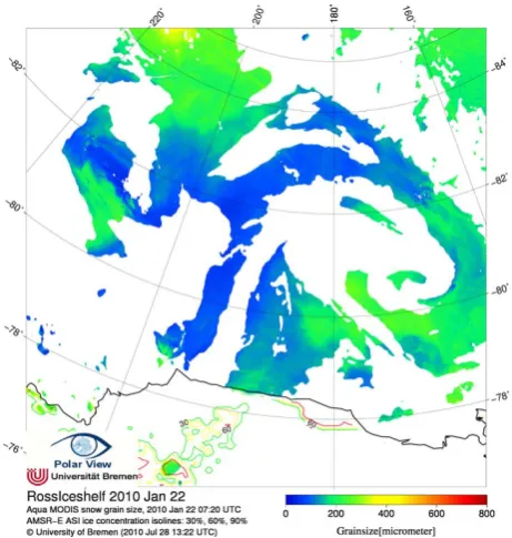
The SGSP includes newly developed iterative atmospheric correction procedure that allows for the real snow BDRF and provides a reasonable accuracy of the snow parameters re-trieval even at the low sun positions typical for polar regions. The SGSP algorithm has been extensively and success-fully validated (Zege et al., 2011; Wiebe et al., 2012) us-ing computer simulations with SRS code. Detailed compar-ison with field data obtained during campaigns carried out by Aoki et al. (2007), where the micro-physical snow grain size was measured using a lens and a ruler, was performed as well (Wiebe at al., 2012). The SGSP-retrieved snow grain size complies well with the in-situ measured snow grain size. The SGSP code with the atmospheric correction proce-dure is operationally applied in the MODIS processing chain providing MODIS snow product for selected polar regions (see www.iup.uni-bremen.de/seaice/amsr/modis.html). Fig-ure 5 shows an example of the operational retrieval of snow grain size on the Ross ice shelf. The large-scale variation of the snow grain size depicted in the figure might be cause by regionally varying meteorological influences like snow depo-sition, as explained in a local study by Wiebe et al. (2012) by comparison of a time series with observations from an auto-mated weather station, and by temperatures reaching nearly melting during this season.

1 2 3

4 Figure 5. Snow grain size retrieval example on the Ross ice shelf as provided in near real time.

41

Fig. 5. Snow grain size retrieval example on the Ross ice shelf as

provided in near real time.

4.2 In situ measurements of snow reflectance

For validation of any remote surface sensing observations from satellite, in situ observations are required. These are dif-ficult to obtain in the high Arctic. The in situ component of the Damocles project has helped to fulfil these requirements with a campaign of 15 scientists, 2 weeks total duration at end of April 2007, to Longyearbyen, Svalbard, and to the schooner Tara drifting with the sea ice (Gascard et al., 2008). The original plan had been to measure the snow reflectance with a Sun photometer CIMEL CE 318 at both places. How-ever, it turned out that the sea ice surface near Tara drift-ing at the time of the campaign near 88◦N was too rough, so that snow reflectance measurements were only taken in Longyearbyen. The observation site was the flat top of a 450 m high hill with few radomes for satellite communica-tions at a distance of several hundreds of meters. The ter-rain was gently sloping towards 5◦W. Taking the reflectance measurements at Longyearbyen as a proxy for those at Tara may introduce two types of errors, namely by differences in roughness and salinity. We assume that the difference in roughness cancels out if considering footprint sizes at satel-lite sensors scales (about 1 km2). Also the difference in snow salinity should be small as at this season the snow cover was about 15 to 25 cm. No indications of seawater flooding of the lower snow layers were found near Tara, and if, then it would have been hardly visible as the penetration depth of sunlight into the snow is clearly less.

G. Heygster: Remote sensing of sea ice: progress from DAMOCLES project 1419 1

2 3

4 5 6 7

Figure 6: The CIMEL sun photometer CE 318 equipped with additional heating and thermal insulation (golden color) during sky observations on the Arctic sea ice near Tara at about 88°N. .

42

Fig. 6. The CIMEL Sun photometer CE 318 equipped with

addi-tional heating and thermal insulation (golden color) during sky ob-servations on the Arctic sea ice near Tara at about 88◦N.

The Sun photometer CIMEL CE 318 had been equipped with two additional heatings and a thermal insulation (Fig. 6) in order to ensure reliable functioning of the electrical and mechanical drive and the electronics under Arctic condi-tions. The photometer is able to observe at 8 wavelengths, of which 6 were used here, namely 340, 440, 500, 670, 870 and 1020 nm. The channels at 380 nm and 940 nm, strongly influenced by calibration problems and water vapour, respec-tively, were not used. Three types of radiance measurements were performed, in the sky along the Sun principal plane and along Sun almucantars, i.e. circles parallel to the hori-zon at the Sun elevation. The surface reflectance in direc-tion towards the Sun and perpendicular to it was also mea-sured. While the sky measurement sequences are ready pro-grammed in the photometer by the provider, the reflectance measurements were realized by an additional metal mirror placed under an angle of 45◦in front of the photometer, de-flecting the incoming radiation by 90◦ from the ground so that the pre-installed Sun principal plane observation pro-gram could also be used for the surface measurements. The opening angle of the photometer of 1.2◦leads at a height of the photometer head of 1.2 m above ground, to a footprint of the sensor on ground varying between 1.3 and 7.2 mm if the observing zenith angles varies from 10 to 80◦.

The snow reflectance at view nadir angles 0 to 80◦was measured on 21 April. Figure 7 and Table 1 show the re-sults from two wavelengths, 440 and 1040 nm. At 440 nm, the reflectance increases from about 0.9 to 1.6 with the view angle towards the Sun increasing from 0◦_{to 80}◦_{. In the} per-pendicular direction, the increase is much slower and reaches only up to about 1.0. In both directions, several curves have been taken. The observed variability of the reflectance can be explained with the small diameter of the footprint, so that different and independent spots are observed from one pho-tometer run to the next. The reflectance at 1020 nm wave-length shows a similar behaviour, but starts at clearly lower

Table 1. Comparison of reflectances taken in situ at Longyearbyen

(this paper), and from space by PARASOL over Greenland and Antarctica (Kokhanvosky and Breon, 2011).

Direction towards Sun Direction perpendicular to Sun

0◦ 60◦ 80◦ 0◦ 50◦ 80◦

1020 nm

Longyeab 0.70 1.20 1.90 0.70 0.80 0.90

Greenland 0.70 0.90 – 0.70 0.72 –

Antarctica 0.65 0.90 – 0.65 0.67 –

(30◦)

670/440 nm

Longyeab 0.90 1.20 1.65 0.90 0.98 1.00

Greenland 0.93 1.05 – 0.92 0.92 –

Antarctica 0.91 1.06 – 0.90 0.91 –

(30◦)

values (∼0.7). The increase in the direction perpendicular to the Sun reaches 0.9 at 80◦view angle, but values are as high as 1.9 towards the Sun.

For a Lambertian surface, the reflectance does not depend on the view angle. In both observing directions we note that surface does not behave Lambertian, but for different rea-sons: towards the Sun, there is an additional broad specular component, which we can interpret as being caused by an orientation distribution of the flat snow crystals on ground with a broad maximum at flat orientation. A purely specu-lar component would have a clear peak at the view angle of the Sun zenith angle, i.e. 72◦_{, broadened by the orientation} distribution of the snow crystals. However, the maximum re-flectance has been observed at 80◦_{view angle. This} discrep-ancy can hardly be explained with the sampling distance of 10◦ view angle. Rather, it may be explained with the glint theory of Konoshonkin and Borovoi (2011) who showed that the width of the peak increases and the viewing zenith angle of the reflectance maximum decreases with the maximum tilt angle of the snow flakes.

In the direction perpendicular to the Sun, the increase of reflectance can be confirmed visually and qualitatively as ex-plained by Fig. 6: the shadows of small-scale roughness in the snow become less visible at more oblique incidence an-gles.

1

2

3

4

Figure 7: Snow reflectance functions taken in Longyearbyen at 1020 nm (left) and 440 nm (right).

Different curves represent different measurements.

43

Fig. 7. Snow reflectance functions taken in Longyearbyen at 1020 nm (left) and 440 nm (right). Different curves represent different

measure-ments.

₁

2

0.2 0.4 0.6 0.8 1.0 1.2 1.4 1.6 1.8 2.0 2.2 2.4 2.6

0.0 0.1 0.2 0.3 0.4 0.5 0.6 0.7 0.8 0.9 1.0



R=0.94exp(-3.5(d)0.5)

re

fl

e

c

ti

on func

ti

on

wavelength, micrometers

theory (d=0.12mm) experiment

Averaged measurements

Model, snow grain size 0.12 mm, SZA= 72.27°

3

4

5

6

7

Figure 8: (a) all observed reflectances, together with those obtained from the snow forward model of

Kohanovsky (2011) with effective grain size 0.12 mm, (b) observed and modelled (Kohknaovsky et al.

2011) snow reflectance.

44

Fig. 8. (a) All observed reflectances, together with those obtained from the snow forward model of Kohanovsky et al. (2011) with effective

grain size 0.12 mm, (b) observed and modelled (Kohknaovsky et al., 2011) snow reflectance.

and perhaps more important, the increase of the reflectance with view angle is in all cases clearly more pronounced in the Longyearbyen observations, and the strong increase of the reflectance beyond 60◦ _{in the direction toward the Sun} is completely missed in the PARASOL observations. On the other hand, the PARASOL observations also cover negative view angles, i.e. in the direction pointing away from the Sun, which have not been taken in situ, so that both observations may complement each other when being used for modelling the snow reflectance.

The reflectances at the various wavelengths (Fig. 8a) can be used to determine the effective grain diameter that best fits the reflectance spectrum. This has been done using the forward model of Kokhanovsky et al. (2011), leading to an effective grain size of 0.122 mm. The reflectances obtained from the forward model with this value are also shown in Fig. 8a and b and show the agreement of the calculated

re-flectance function with the observations, at least in the wave-length range up to 1020 nm.

4.3 Snow albedo

Currently the snow albedo is found using several satellite in-struments. Routine visible satellite observations of the po-lar regions began in 1972 with launch of the first Landsat. The NOAA/AVHRR sensor provides the longest time se-ries of surface albedo observations currently available. The AVHRR Polar Pathfinder (APP) (Fowler et al., 2000) prod-uct is available from the National Snow and Ice Data Cen-ter (http:/nsidc.org), providing twice daily observations of surface albedo for the Arctic and Antarctic from AVHRR spanning July 1981 to December 2000. The accuracy of this product is estimated to be approximately 6 % (Stroeve et al., 2001). In addition, Riihel¨a et al. (2010) performed the val-idation of Climate-SAF surface broadband albedo using in

G. Heygster: Remote sensing of sea ice: progress from DAMOCLES project 1421

0.40 0.45 0.50 0.55 0.60 0.65 0.70 0.75 0.80 0.85 0.90 0.0

0.1 0.2 0.3 0.4 0.5 0.6 0.7 0.8 0.9 1.0

al

bedo

wavelength, micrometers

May 3 April 28 March 31

Figure 9. The albedo retrieved from MERIS observations for several days in 2006 (average for all orbits). As it should be, albedo decreases with the wavelength and it is smaller for days with higher temperature. The results for the point wit

1 2

h the coordinates (24.6E, 79.8N) is given (glacier Austfonna, 3

island Nordaustlandet on Spitsbergen ). 4

45

Fig. 9. The albedo retrieved from MERIS observations for several

days in 2006 (average for all orbits). As it should be, albedo de-creases with the wavelength and it is smaller for days with higher temperature. The results for the point with the coordinates (24.6◦E, 79.8◦N) are given (glacier Austfonna, island Nordaustlandet on Spitsbergen).

situ observations over Greenland and the ice-covered Arctic Ocean, and the seasonality of spectral albedo and transmis-sivity of sea ice were observed during the Arctic Transpolar Drift of the Schoner Tara in 2007 (Nicolaus et al., 2010). A prototype snow albedo algorithm for the MODIS instrument was developed by Klein and Stroeve (2002). Models of the bidirectional reflectance of snow created using a discrete or-dinate radiative transfer (DISORT) model are used to correct for anisotropic scattering effects over non-forested surfaces. Maximum daily differences between the five MODIS broad-band albedo retrievals and in situ albedo are 15 %. Daily dif-ferences between the “best” MODIS broadband estimate and the measured SURFRAD albedo are 1–8 %. Recently, Liang et al. (2005) developed an improved snow albedo retrieval algorithm. The most important improvement to the direct re-trieval algorithm is that the nonparametric regression method (e.g. neural network) used in the previous studies has been replaced by an explicit multiple linear regression analysis. Another important improvement is that the Lambertian as-sumption used in the previous study has been replaced with a more explicit snow BRDF model. A key improvement is the inclusion of angular grids that represent reflectance over the entire Sun-viewing angular hemisphere. A linear regression equation is developed for each grid, and thus thousands of linear equations are developed in this algorithm for convert-ing TOA reflectance to surface broadband albedo directly.

The shortcoming of methods described above is the use of an assumption that the snow grains have a spherical shape. Therefore, we have developed an approach that is based on the model of aspherical snow grains. In particular we have used the following equation for snow reflectance functionR

(Zege et al., 1991):

R=R0Ap. (1)

Here, A is the snow albedo, R0 is the snow reflec-tion funcreflec-tion for the nonabsorbing aspherical grains (pre-calculated values are assumed for fractal snow grains),p=

K (µ0) K (µ) /R0, K (µ)=3₇(1+2µ) , µis the cosine of the observation zenith angle and µ0 is the cosine of the so-lar zenith angle. The atmospheric correction is applied to satellite data for the conversion of satellite – measured re-flectance Rsat to the value of snow reflectanceR. Such an approach was validated using ground measurements (Negi and Kokhanovsky, 2010) and found to be a robust and fast method to derive snow albedo with account for the snow BRDF. We note that Eq. (1) can be used directly to find the snow albedo:

A=(R/R0)1/p. (2)

The results of retrievals for Spitzbergen are given in Fig. 9. They are based on measurements of MERIS (MEdium Res-olution Imaging Spectrometer) on board ENVISAT. Valida-tion of the albedo retrievals can be done indirectly using the extensively validated grain size (Wiebe et al., 2012; Kokhan-vosky et al., 2011).

5 Sea ice drift and deformation

The dynamic Arctic sea ice transports fresh water, its im-port contributes negatively to the latent heat budget, and it strongly influences the heat flux between ocean and atmo-sphere through opening and closing of the sea ice cover (Maykut, 1978; Marcq and Weiss, 2012). Sea ice dynamics also contribute to the ice thickness distribution through ridg-ing and raftridg-ing. Thermodynamic ice growth leads to maxi-mum thickness of about 3.5 m for multi-year ice (Eicken et al., 1995), higher thickness are typically generated by dy-namic processes.

Table 2. Main characteristics of the ice drift data sets available from the Damocles project. Grid Spacing: spacing between ice motion vectors;

Time Span: duration of the observed motion; Area Averaging: extent of the area of sea ice that is monitored by each motion vector; Data set Coverage: the period for which the data is available; Annual Coverage: the time of year in which ice drift data are produced.

Product Source Instrument/ Grid Time Area Data set Annual

Institution Mode Spacing Span Averaging Coverage coverag

OSI-405 OSI SAF SSM/I, AMSR-E, 62.5 km 48 h ∼140×140 km2 2006-ongoing Oct–May ASCAT

IFR-Merged CERSAT/ SSM/I, QuikSCAT, 62.5 km 72 h ∼140×140 km2 1992-ongoing Oct–May IFREMER ASCAT

IFR-89 GHz CERSAT/ AMSR-E 89 31.25 km 48 h ∼70×70 km2 2002–2011 Oct–May IFREMER GHzH /V

OSI-407 OSI SAF AVHRR band 2/4 20 km 24 h ∼40×40 km2 2009-ongoing All year DTU-WSM DTU ASAR-WSM 10 km 24 h ∼10×10 km2 2010–2012 All year

All four ice drift products are developed jointly between the DAMOCLES project and other national and international projects.

Present ice drift products consist of sea ice displacement vectors over some period of time (T toT +dT) and for an area defined by the product grid size, the latter ranging be-tween 10 and 100 km and dT ranging bebe-tween 12 h and 3 days. The ice drift data contain no details of the sea ice during the displacement period,dT. Hence, a complete description of the sea ice dynamics requires high temporal and spatial resolution. However, a general condition of Earth observa-tion data with satellites is that a tradeoff exists between tem-poral coverage and spatial resolution. Some data sets pro-vide high temporal resolution; some propro-vide very good spa-tial coverage whereas others provide only parspa-tial coverage of the Arctic. Some data sets are available only during winter months whereas others are available all year around. These are the reasons why it takes several different ice drift data sets to get detailed knowledge of sea ice dynamics on a broader range of spatial and temporal scales. Methods to relate data sets with different sampling characteristics have been sug-gested by, e.g. Rampal et al. (2008) from an analysis of drift-ing buoy dispersion. They found a power law relation be-tween the temporal and spatial deformation.

Through the past decade drastic changes of the sea ice drift and deformation patterns in the Arctic Ocean have been re-ported in various studies (Vihma et al., 2012; Spreen et al., 2011; Rampal et al., 2009). These changes coincide with co-herent reports on decreasing Arctic sea ice volume and gen-eral thinning of the ice cover (Kurtz et al., 2011; Kwok, 2011; Rothrock et al., 2008). The great loss of Arctic sea ice dur-ing the ice minimum in 2007 seem to have had a particular strong impact on the ice drift patterns, and especially the loss of large amounts of perennial sea ice in the Western Arc-tic seems to have changed the sea ice characterisArc-tics there (Maslanik et al., 2011). New results of drift and deforma-tion characteristics in the Western Arctic are presented in Sect. 5.5. This analysis is based on ice drift and deformation

data calculated from the full data set of AMSR-E passive mi-crowave data from 2002 to 2011. These drift and deformation data constitute to our knowledge the most accurate and con-sistent daily and Arctic-wide data set covering this period. 5.1 ASCAT and multi-sensor sea ice drift at

IFREMER/Cersat

Like SeaWinds/QuikSCAT, the scatterometer ASCAT is pri-marily designed for wind estimation over ocean. It is a C-band radar (5.3 GHz) like two precursors on the European Research Satellites ERS-1 and ERS-2, respectively, hence-forth together denoted as ERS. Like ERS, the ASCAT ob-serving geometry is also based on fan-beam antennas. Over sea ice, the backscatter is related to the surface roughness of ice (at the scale of the wavelength used), which in turn is linked with ice age (Gohin, 1995). In contrast to open wa-ter, the backscatter is not a function of the azimuth of the beam but varies strongly with incidence angle. As a con-sequence, swaths signatures are clearly visible in ASCAT backscatter data, indicating that such data cannot be used di-rectly for geophysical interpretation. It is indeed mandatory to construct incidence-adjusted ASCAT backscatter maps for sea ice application. It is noteworthy that the backscatter from SeaWinds/QuikSCAT scatterometer does not require an inci-dence angle correction because of its conically revolving an-tennas providing constant incidence angle. Based on the ex-perience from ERS and NSCAT data, IFREMER has devel-oped algorithms to compute incidence-adjusted backscatter maps normalized to 40◦_{incidence angle. Once corrected, the} backscatter values over sea ice can be further interpreted with horizontally homogeneous retrieval algorithms in order to detect geophysical structures which can be compared to those from SeaWinds/QuikSCAT maps. ASCAT offers a complete daily coverage of the Arctic Ocean, although some peripheral regions are not entirely mapped each day (e.g. Baffin Bay).

One application of the ASCAT incidence-adjusted backscatter maps is to estimate sea ice displacement. Al-though single ice floes cannot be detected with the low pixel

G. Heygster: Remote sensing of sea ice: progress from DAMOCLES project 1423

resolution available with microwave sensors such as ASCAT (typically 10–20 km), the general circulation of sea ice can effectively be mapped on a daily basis. Several motion ex-traction methods have been tested based on tracking com-mon features in pairs of sequential satellite images. The most commonly used technique, the Maximum Cross Correlation (MCC), enables only detection of translation displacement (Kamachi, 1989; Ninnis et al., 1986). The main limitation of the MCC is the angular resolution for small drifts: the vec-tor direction in slow motion areas has a larger uncertainty. A correlation is estimated between an array of the backscat-ter/brightness temperature map in one day and an array of the same size of another map separated in time. In particu-lar, Girard-Ardhuin and Ezraty (2012) apply this process on the Laplacian field in order to enhance the structures to be tracked. The relative location of the maximum similarity be-tween the arrays of the two original images is the displace-ment vector. To remove outliers, a threshold minimum corre-lation coefficient is imposed, and a comparison with the wind pattern is often applied (ECMWF model for Girard-Ardhuin and Ezraty, 2012; NCEP re-analyses for Kwok et al., 1998) since mean sea ice drift is strongly linked with geostrophic winds.

Brightness temperature maps from passive microwave ra-diometers have been used for sea ice drift estimation since the 1990s. The same method has been applied to scatterom-eter data, first with 12.5 km pixel resolution one day aver-age SeaWinds/QuikSCAT backscatter maps and now with ASCAT (same grid resolution). This allows to process ev-ery day during winter, 3- and 6-day lag ice drift maps since 1992 with radiometers (SSM/I, AMSR-E) and scatterome-ters since 1999 with SeaWinds/QuikSCAT and ASCAT. The noise level is dominated by sensor ground resolution and pixel size. Advantages and shortcomings of each product de-pend on pixel sizes, period and magnitude of drift.

One recent major improvement of these drift estimations is the combination of two drift fields (QuikSCAT with SSMI and now ASCAT with SSMI): it provides better confidence in the results than each individually since each drift is in-ferred from independent measurements. The number of valid drift vectors is increased, in particular for early fall and early spring (more than 20 %), and the merged drift enables dis-crimination of outliers remaining in the individual products (Girard-Ardhuin and Ezraty, 2012). A time and space inter-polation algorithm has been added to fill the gaps and pro-vide the fullest field as possible, as often requested by the modelling community. The CERSAT/IFREMER backscatter and sea ice drift time series since 1992 is ongoing for Arctic long term monitoring with the Metop/ASCAT scatterometer data. Data are easy and free to access via the CERSAT portal (http://cersat.ifremer.fr). The merged sea ice drift products have been validated against buoys, and the standard devia-tion of the difference ranges from 6.2 to 8.6 km, depending on the sensors and the day-lags used, including 5.1 km due

to quantification effect (Girard-Ardhuin and Ezraty, 2012). Characteristic values of products are found in Table 2.

A recent study has made the effort to compare drift data sets at several resolutions from models, in situ and satellite observations in the particular area of the Laptev Sea, show-ing that the satellite-inferred drifts (those presented here and in Sect. 5.4) present good estimates; in particular the CER-SAT/IFREMER product (Ifremer-89 GHz) has an especially strong correlation and low standard deviation compared to the reference data (Rozman et al., 2011).

5.2 Sea ice drift from AVHRR observations

For the DAMOCLES project, a MCC sea ice motion retrieval algorithm was developed for data from the Metop/AVHRR instrument. The setup operates on swath data at original spa-tial resolution (approximately 1 km) of visible (VIS, channel 2) and Thermal InfraRed (TIR, channel 4) data. The VIS data are used during sunlit periods, when the TIR data show poor applicability for feature recognition as a consequence of low temperature difference between snow/ice interface and water. The TIR data are thus used during autumn, winter and spring, when leads, ridge zones and thin ice are easily recognised in the data. Characteristics of the setup are found in Table 2.

The use of satellite based VIS and TIR measurements for sea ice drift retrievals is limited by the presence of clouds, so the applicability is therefore constrained to areas below clear skies. This limitation, in combination with comprehensive filtering for dubious ice displacement vectors, causes large data gaps, especially during the Arctic summer when cloud cover prevails. However, the advantage of using AVHRR data for ice drift monitoring is the daily coverage of the Arctic re-gion with high spatial resolution, providing high precision ice drift estimates. A comparison of this product to high pre-cision GPS buoy positions shows that the standard deviation of the 24 h displacement error is around 1 km in both summer and winter (Hwang and Lavergne, 2010).

The AVHRR ice motion product is suited for data assim-ilation and for tuning of model ice parameters, like sea ice strength, thanks to its fine temporal and spatial resolution, as well as the high product accuracy. The product should also prove useful for validation of modelled sea ice motion. This 24 h ice motion product has subsequently been opera-tionalized and is now available from the OSISAF web por-tal, where further documentation of the product is available (http://osisaf.met.no).

5.3 Sea ice drift from ASAR observations

2

A: B:

C: D:

46

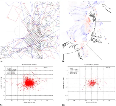
Fig. 10. (A) Example of ice drift derived from ENVISAT ASAR WSM data between 15 March and 16 March 2010. Only every 25th vector

shown. Red rectangles show ENVISAT WSM coverage on 15 March, blue on 16 March. (B) Example of corresponding ice deformation pattern derived by differentiating the ice drift field between 15 and 16 March 2010. Blue shows areas of divergence and red areas of conver-gence. (C) Validation of ice ENVISAT ASAR derived ice drift against hourly GPS locations from Ice Tethered Platforms (spring). Axes are difference in drift in 24 h (in km). (D) Validation of ice ENVISAT ASAR derived ice drift against hourly GPS locations from Ice Tethered Platforms (summer).

images. In 2002, ESA launched the Envisat satellite with its Advanced Synthetic Aperture Radar (ASAR) instrument, wherewith the data coverage increased tremendously. After the release of the coarse resolution (1000 m) Global Monitor-ing Mode (GMM) images in 2004, ice feature trackMonitor-ing from these images was developed at the Danish Technical Uni-versity (DTU). The method is similar to the RGPS method, i.e. maximizing a two dimensional digital cross correlation (MCC) to find matches between images 3 days apart. Drift vectors every 20 km were derived, and the method proved skills in deriving ice drift even during the summer months where most other methods fail. In June 2007, ESA started providing much improved coverage of the polar regions, now in the finer resolution (150 m) Wide Swath Mode (WSM). Daily coverage of the European sector of the Arctic has been available almost continuously since 2007. The DTU

pro-cessing scheme was adapted to the higher resolution WSM scenes, and a data set of daily ice drift vectors from June 2007 to the present is being continuously updated, now as part of the EU MyOcean project. The individual 150 m resolution data-files are averaged and gridded to a polar stereographic projection at 300 m grid spacing, and ice features are tracked using circular subsets of 5 km radius sampled every 10 km. Each swath of day 1 is correlated with each overlapping swath of day 2, which are separated in time by between 12 and 36 h (Table 2). The processing provides very accurate ice drift vectors from the coverage area (RMS difference to GPS buoys less than 500 m in 24 h, see Fig. 10c and d). Mode de-tailed validation with GPS drift buoys show RMS uncertain-ties of between 200 m and 600 m for the 12–36 h drift vec-tors, depending somewhat on area and season (Hwang and Lavergne, 2010). This is substantially better than most other

G. Heygster: Remote sensing of sea ice: progress from DAMOCLES project 1425

ice drift products. The coverage is generally limited to the area of the Arctic Ocean between 90◦_{W and 90}◦_{E (see} ex-ample in Fig. 10a). ENVISAT ASAR coverage only extends to approximately 87◦N. The ASAR ice drift data set can be derived all year round contrary to most other data sets (see Fig. 10d).

5.4 Multi-sensor ice drift analysis at the EUMETSAT OSI SAF

All ice drift products described previously in this chapter are based on the MCC algorithm. However, it exhibits strong weaknesses when the length of the displacement is short with respect to the pixel size. For example, displacements that are less than half an image pixel in length cannot be retrieved and are identified as zero-drift. For the same rea-son, the angular resolution of the motion vector field is poor for short displacement lengths. This noise is often referred to as the quantization noise or tracking error. While this does not restrict the usefulness for motion tracking from high-resolution images (e.g. SAR, Sect. 3) or AVHRR (Sect. 5.2), the quantization noise is largely apparent in MCC-based mo-tion vector fields from low-resolumo-tion images acquired by passive microwave instruments such as SSM/I, and AMSR-E and scatterometers such as QuikSCAT/SeaWinds and AS-CAT (Sect. 5.1).

An alternative motion tracking method was thus devel-oped during the DAMOCLES project. The Continuous MCC (CMCC, Lavergne et al., 2010) is strongly linked to the MCC, but uses a continuous optimization step for finding the motion vector that maximizes the correlation metric. As a re-sult, the quantization noise is removed, and the motion field obtained from the low-resolution images is spatially smooth and does not exhibit the MCC artefacts such as zero-length vectors and poor angular resolution. Particularly, the defor-mation metrics such as the convergence/divergence are more realistic from a field processed by the CMCC than by the MCC (see Sect. 5.5).

The CMCC was successfully applied to ice motion track-ing from AMSR-E (37 GHz), SSM/I (85 GHz), and ASCAT daily images (12.5 km grid spacing). Validation against GPS buoys document un-biased and accurate estimates, with stan-dard deviation of the error in x- and y-displacement ranging from 2.5 km to 4.5 km after 48 h drift, depending on the in-strument used. In any case, these validation statistics were documented to be better than those obtained from the same satellite sensors, even with using the more crude MCC tech-nique (Sect. 4.3 in Lavergne et al., 2010).

The ice drift algorithms of Lavergne et al. (2010) were implemented in the operational processing chain of the EUMETSAT OSI SAF in late 2009. Daily products (OSI-405, both single- and multi-sensor, Table 2) are available from the OSI SAF web site (http://osisaf.met.no) for use in sea ice monitoring and data assimilation by coupled ocean and ice models (Lavergne and Eastwood, 2010).

5.5 Sea ice deformation

Sea ice drift and deformation generate leads, ridges and fault-ing in the sea ice cover with subsequent exposure of open wa-ter to the atmosphere, thus significantly increasing the trans-port of heat and humidity from the ocean to the atmosphere, as mentioned above. The ice drift speed and the degree of deformation depends on the main forcing parameters, wind and ocean current, and on the internal strength of the ice.

Thin ice deforms easier than thick ice (Kwok, 2006; Ram-pal et al., 2009; Stern and Lindsay, 2009). Ice deformation characteristics therefore function as a proxy for ice thickness and thus as an indicator of the state of sea ice, provided that wind and ocean forcing is even.

There are no simple and unambiguous trends in the sur-face wind patterns over the Arctic Ocean in recent years, and trends seem to depend on both season and region. Smed-srud et al. (2011) analyzed NCEP/NCAR reanalysis data and found that wind speeds have increased southward in the Fram Strait throughout the past 50 yr and increasing the ice export here. Also using NCEP/NCAR reanalysis data, Hakkinen et al. (2008) report increasing storm activity over the central Arctic Ocean in the past 50 yr, resulting in positive trends of both wind stress and ice drift. Spreen et al. (2011) analyzed four different atmosphere reanalysis data sets for nearly two decades, up to 2009. Their analysis showed large regional differences, with areas of both negative and positive wind speed trends across the Arctic Ocean. However, both Vihma et al. (2012) and Spreen et al. (2011) found that the positive trends in sea ice drift during the past 2 decades cannot be explained by increased wind stress alone. This study shows no positive trends in wind speeds for the ice covered Arctic Ocean since 2002 (see Fig. 12).

More than 70 % of the short term ice drift is explained by geostrophic wind (Thorndyke and Colony, 1982), thus leav-ing only a small fraction of the ice drift to surface current and internal stress. Therefore we assume that trends in the Arctic surface currents in the past decades have negligible influence on the changing characteristics of the Arctic sea ice dynam-ics. Rather we assume that the graduate thinning of the Arctic sea ice in recent years is the main cause for changing ice drift and deformation characteristics. This is also documented in several studies, e.g. Vihma et al. (2012), Spreen et al. (2011) and Rampal et al. (2009).

1 2 3 4 5 6 7 8

Figure 11: Monthly mean values of Western Arctic 48 hour sea ice divergence (black lines and circles) and convergence (grey lines and circles), during seven winter month (Oct-May) since 2002. Mean values are based on daily divergence fields calculated from AMSR-E ice drift fields, using the CMCC algorithm. The ice convergence values are negative divergence values, but plotted here as absolute values for comparison to positive divergence values. The associated diverged and converged areas are plotted as aggregated winter (Oct-May) values in square kilometres (black and grey triangles, respectively).

48

Fig. 11. Monthly mean values of Western Arctic 48 h sea ice divergence (black lines and circles) and convergence (grey lines and circles),

during seven winter month (October–May) since 2002. Mean values are based on daily divergence fields calculated from AMSR-E ice drift fields using the CMCC algorithm. The ice convergence values are negative divergence values, but plotted here as absolute values for comparison to positive divergence values. The associated diverged and converged areas are plotted as aggregated winter (October–May) values in square kilometres (black and grey triangles, respectively).

1 2

3 4 5 6 7 8 9

Figure 12: Monthly mean ice/wind speed ratios, November 2002 to March 2012, from the Western Arctic regions. The red line is fitted to October-November-December data and the black line is the fitted line to all data (red and black), with levels of significance at 0.11 and 0.06, respectively. The grey points with error bars are monthly mean wind speed with ±1 Standard deviation.

49

Fig. 12. Monthly mean ice/wind speed ratios, November 2002 to March 2012, from the Western Arctic regions. The red line is fitted to

October-November-December data and the black line is the fitted line to all data (red and black), with levels of significance at 0.11 and 0.06, respectively. The grey points with error bars are monthly mean wind speed with ±1 Standard deviation.

export and melt area during summer as the dominating anti-cyclonic rotation now exports MYI into the open water where it melts during summer. This is a very significant change in the sea ice of the Arctic Ocean in recent years. The ice drift and deformation results discussed below focus on the West-ern Arctic sea ice, as the largest changes are anticipated to emerge here.

An ice drift and deformation data set, based on the full time series of AMSR-E data (from 2002 to 2012), was ana-lyzed for changing characteristics in the Western Arctic sea ice behaviour. The AMSR-E ice drift data set was produced using the CMCC methodology mentioned in Sect. 5.4. Ice divergence fields are produced from the highest quality and non interpolated drift vectors to ensure best quality data. The

divergence is calculated as the area change of a grid cell (Dy-bkjaer, 2010). The uniqueness of this ice drift and divergence data set lies in the combination of high precision, daily Arc-tic coverage, high data consistency through the single sensor status and the fact that it covers the most dramatic changes in sea ice characteristics in recent years.

Sea ice divergence and convergence data for the Western Arctic Ocean are shown in Fig. 11 as mean monthly values. Mean divergence is estimated for all areas with a positive area change (opening of leads) and mean convergence is es-timated for all areas with a negative area change (ridging and rafting) over 48 h. An annually consistent feature in the data is the relative high deformation rates in the month after the summer melt period when large areas are covered by new