Decentralized Advanced Model Predictive Controller
of Fluidized-Bed for Polymerization Process
Ahmmed S. Ibrehem*+
Department of Chemical Engineering, UiTM University of Mara 40450 Shah Alam, MALAYSIA
Mohamed A. Hussain
Department of Chemical Engineering, University of Malaya 50603 Kuala Lumpur, MALAYSIA
Nayef M. Ghasem
Department of Chemical Engineering, University of Al Ain. U.A.E
ABSTRACT: The control of fluidized-bed operations processes is still one of the major areas of research due to the complexity of the process and the inherent nonlinearity and varying dynamics involved in its operation. There are varieties of problems in chemical engineering that can be formulated as NonLinear Programming (NLPs). The quality of the developed solution significantly affects the performance of such system. Controller design involves tuning the process controllers and implementing them to achieve certain performance of controlled variables by using Sequential Quadratic Programming (SQP) method to tackle the constrained high NLPs problem for modified mathematical model for gas phase olefin polymerization in fluidized-bed catalytic reactor. The objective of this work is to present a comparative study; PID control is compared to an advanced neural network based MPC decentralized controller and also, see the effect of SQP on the performance of controlled variables. The two control approached were evaluated for set point tracking and load rejection properties giving acceptable results.
KEY WORDS:Model predictive control, Proportion integral derivative control, Neural networks, Optimization.
INTRODUCTION
The incentive for process control may vary depending on the processes application under consideration. The objectives include; maintaining high product quality, avoiding or minimizing losses, maximizing throughput, minimizing operational costs, and ensuring safe and an environment friendly operation. Furthermore, studying the control of fluidized-bed, polymerizations operations
has always been a research active area because of its complexity and non-linearity that obscure the design of optimum control strategies capable of handling the whole ranges of operation. This is further complicated by the availability of a variety of contacting geometries, and the use of diverse processing techniques. The processes entailed in fluidization are highly complex and often
*To whom correspondence should be addressed.
+E-mail: [email protected]
require extensive coordination and management in order to ensure that they are handled efficiently and with high safety standards. The ability of the process to achieve and maintain the desired equilibrium value is termed as the controllability of the process. This is measured by considering a range of properties of the non linear process [1]. However, in engineering practice a plant is called controllable if it is possible to achieve the specified control objectives [47]. Control strategy involves the design of control systems and studying them for stability and robustness. Controller design involves tuning the process controllers and implementing them to achieve certain performance of controlled variables. Nevertheless, most industrial polymerization processes are still controlled using linear controllers based on linear process model. However starting from the last decade, some researchers [31],[5],[13] have started proposing nonlinear controller designs to control certain severely nonlinear processes where tight control is required. Furthermore, most of the nonlinear control problems related to polyethylene reactors are highly complex. This process is represented one of the major challenges facing process engineers in the chemical process industries and this process requires optimization and control of product quality while keeping process variable costs as low as possible.
Modern control algorithms attempt to address these difficulties and to solve the polymerization control problem under variable operating conditions in order to achieve optimal performance. Many such algorithms have been proposed during the last two decades [2].
Recently, the Model Predictive Control (MPC) has attracted researchers as well as process engineers to implement it as one of the most recommended advance process algorithms, both in academic and industry. The combination of new control design concepts in MPC, such as model predication, receding horizon optimization and real time correction, makes it possible to yield high performance characteristics and Neural Network (NN) based control system design is gaining a great deal of attention due to the networks universal approximation ability, on and off learning feature, and their parallelism [4],[6].
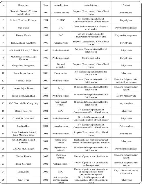
Control studied for the polyethylene production process spans a variety of schemes and algorithms. A list of relevant studies is given in Table 1 for the period 1990-2008 [8].
In this work, we have utilized the advantages of both methods within a neural-network model based model
prediction controller to control the fluidized bed polyethylene reactor. The model used for the control is the modified model developed recently by [1]. Control studies were done for set point tracking and disturbance rejection and comparison made with the PID controller.
THEORITICAL SECTION
Descriptive behavior of the new mathematical model Heterogeneous models are used widely especially in polymerization system. Current research in this important area can be divided into two parts namely; mathematical models for fixed bed catalyst reactor systems and mathematical models for fluidize bed catalytic reaction for production of polyethylene [29],[71],[23] improved
the heterogeneous model however, they
did not consider solid phase effect. Varma, 1981 included mixing in the axial direction. R. Sala, F. Valz-Gris & L. Zanderighi Paterson developed a two dimensional mathematical model where concentration and temperature patterns in the reactor can be predicted [11],[12].
R.J. Zeman & N. R. Amundson, Xuejing Zheng, Makarand S. Pimplapure, Günter Weickert, and Joachim Loos, Victor M. Zavala, Antonio Flores-Tlacuahuac and Eduardo Vivaldo-Lima improved the Dynamic optimization of a semi-batch reactor for polyurethane production,
H. Hatzantonis, H. Yiannoulakis, A. Yiagopoulos,
C. Kiparissides further improved the two phase model of the polymerization system. In previous works, mass transfer with chemical reaction in fluidized-bed systems either consider all phases (D. Kunii & O. Levenspiel, 1969) or the emulsion phase alone [31],[5],[13].
Modified modeling is by including the catalyst phase and considering all three phases as compared to the other models i.e, constant bubble size model, well mixed model and the bubble growth model. Simulations were also performed to study the effect of superficial velocity and catalyst flow rate in the bubble and emulsion phases. Comparisons with actual plant data at steady state were also performed [1],[17].
Table 1: Summary of control studies for polymerization processes from 1990 to 2008.
No Researcher Year Control system Control strategy Product
1 Elnashaie, Gonzales Velasco,
Abdel-Hakim 1990 Deadbeat method
Set point (Temperature) effect of batch
reactor Polyethylene
2 G. Ravi, Y. Arkun, F. Joseph 1994 NLMPC Set point (Temperature and
Concentration) effect of batch reactor Polyethylene
4 Wei, Danial 1996 IMC Control relevant reduction of volterra
series models Polymerization process
6 Thomas, Francis 1997 IMC An anti-windup scheme for
multivariable nonlinear systems Polymerization process
7 Tian,y.J.Zhang, A.J.Morris 1999 Neural network Set point (Temperature) effect of batch
reactor Polyethylene
8 A.Bolsoni,E.L.Lima, J.C.Pinto 1999 Predictive control Set point (Concentration) effect of
batch reactor Polystyrene
9 Morimasa, Masahiro, Koji,
Fuminao 1999 Predictive control Control melt index Polyethylene
10 Gangadhar, Evanghelos 1999 Optimal
controller
Set point (Temperature) effect of batch
reactor Polystyrene
11 Janos, Lagos, Ferenc 2000 Fuzzy control Set point (Temperature) effect for
batch reactor Polystyrene
12 Yaohui, Yaman 2000 Predictive control Set point (Concentration) effect of
batch reactor
Emulsion Polymerization system of polystyrene
13 Janson, Lajos, Ferenc 2000 Fuzzy Distributed (Temperature) effect for
batch reactor
Emulsion Polymerization system
14 Boong, Goon, Kee, Hyun 2001 Predictive control Distributed (Temperature) effect for
batch reactor Methyl Methacrylate
15 W.C.Chen, Ni-Bin. Chang, Jenj 2001 Fuzzy neural
control
Distributed (Temperature) effect for
batch reactor polypropylene
16 Boong, Kee, Hyu 2001 MPC Set point (Temperature and
Concentration) effect of batch reactor Polystyrene
17 O. Abel, W. Marquardt 2001 Predictive control Set point (Temperature and
Concentration) effect of batch reactor Polystyrene
18 Joachim Horn 2001 Neural network Set point (Temperature and
Concentration) effect of batch reactor Polypropylene
19 Hiroya, Morimasa, Satoshi,
Kouji, Masahiro, Wang 2001 Predictive control
Set point Temperature effect of batch
reactor Polyethylene
20 Robert, Douglas, Ronald,
Babatund 2001
Voletra series model
Identification of nonlinear empirical
models for chemical dynamic processes Polystyrene
21 C.W.Ng, M.A.Hussain 2002 Hybrid neural
network
Distributed (Temperature) effect for
batch reactor Polymerization process
22 Charles, Francis 2002 Open loop
optimal Control of particle size distributaries
Emulsion Polymerization system
23 Yuan, Jie, Julian 2002 Optimal control Control of particle size distributaries
and composition
Emulsion Polymerization system
24 Dulce, Nuno 2002 MPC
Control of particle size distributaries and composition of batch
polymerization system
Vinyl chloride and methyl methacrylate
25 Sang, Hyun 2002
Auto-regressive moving average
model
Set point (Temperature and Concentration) effect of continuous
system
Table 1: Continued
26 Chiaki, Jinyoung 2002 Neural network Set point (Temperature effect of batch
reactor system
Emulsion Polymerization system
27 Nayef Mohamed Ghasem 2005 Optimal control Distributed (Temperature) effect for
batch reactor
Emulsion Polymerization system
28 Zhihua, Jie 2004 Optimal control Batch-to –Batch control Poly Methyl methacrylate
29 Nido, Gilles, Timothy 2003 MPC Set point (Concentration) effect of
batch reactor linear system Polystyrene
30 Kenneth, Ahmet 2003 IMC Control for nonlinear process change in
set point concentration Polystyrene
31 Francis, Christopher, Timothy 2003 MPC Control of particle size distribution in
batch reactor Emulsion Polymerization
32 R.A.M. Vieira, M. Embirucu,
C. Sayer, Lima 2003 MPC
Control of particle size distribution in
batch reactor set point concentration Polystyrene
33 C.Chatziduksa, J. D Perkins,
C. Kiparissides 2003 Optimal control
Set point (Concentration) effect of
fluidized bed reactor Polyethylene
34 D. Del Vecchio, N. Petit 2005 Optimal control Control for tubular chemical reactor Polystyrene
35 Antonio, Lorenz 2005 Optimal control Control for unstable polymerization
reactors Polystyrene
36 G. Mourue, D. Dochain,
V.Wertz, D. Descamps 2004 MPC
Distributed concentration effect for
nonlinear chemical processes Polystyrene
37 Z. Zeybek, S. Yuce, H.Hapoglu,
M. Alpbaz 2004
Adaptive controller
Control heuristic temperature of batch
reactor Polystyrene
38 Dennis, Okko 2005 Predictive control
Distributed (Temperature and concentration) effect for continuous
nonlinear chemical processes
Polyethylene
39 Costas Kiparissides 2005 Optimal control Control on molecular weight
distribution Polyethylene
40 Simant, Baranitharan, Ali 2005 Optimal control
Control for determination of MMA polymerized in non-isothermal batch
reactor
Poly Methyl methacrylate
41 Ch. Vekates, K. Venkat 2005 Neural network Control of unstable nonlinear processes Poly Methyl methacrylate
42 Jesus, Cerrillo, John 2005 MPC Distributed (Temperature and Pressure)
effect for autoclave process
Nylon polymerization autoclave process
43 Babatunde, Ogunnaike, Kapil 2006 MPC Control of nonlinear processes Polystyrene
44 Bassam, Jose 2006 Optimal control Control on emulsion copolymerization
of styrene Poly Styrene
45 B.Alhamad, R. WIillis, J. A.
Romagnoli, Gomes 2006 Optimal control
Control on molecular weight
distribution Poly Styrene
46 Felix, Masound, Michael 2006 Optimal control Control of high temperature semi batch
reactor Poly butyl acrylate
47
Ahmmed s ibrehem, Mohamed Azlan Hussain, Nayef Mohamed
Ghasem
2007 NMPC Control of emulsion temperature and
molecular weight Poly ethylene
48
Sebastian Terrazas-Moreno, Antonio Flores-Tlacuahuac, and
Ignacio E. Grossmann
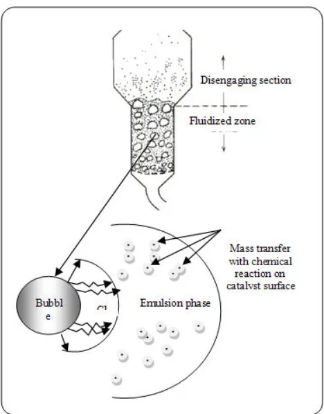
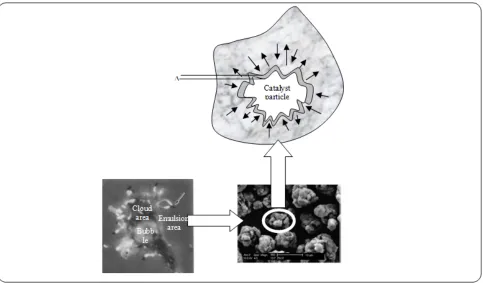
Fig. 1: Steps of polymerization process.
on the surface of catalyst particles, and specify the kind of catalyst particles if the catalyst porous or rigid kind because the kind of catalyst particles has big effects on the rate of reaction. All details can be shown in [1],[17].
In this model the reactant gas enters the bottom of the bed and flows up the reactor in the form of bubbles. As the bubbles rise, mass transfer of the reactant gases takes place between the bubbles and the clouds without chemical reaction, and between the clouds and the emulsion without chemical reaction, and between emulsion and solid with a chemical reaction that happens on the surface of catalyst particles. The model accounts the effects of solid phase on the rate of reaction as shown in Fig. 1.
The product then flows back into the bubble and finally exits the bed when the bubble reaches the top of the bed. The rate at which the reactants and products transfer in and out of the bubble affects the conversion but the time delay of bubble is very small.
The bubbles contain very small amounts of solids. They are not spherical; rather, they have an approximately hemispherical top and a pushed-in bottom.
Each bubble of gas has a wake which contains a significant amount of solids [35],[54],[55].
As the bubble rises, it pulls up the wake with its solids behind it. The net flow of the solids in the emulsion phase must therefore be downward. The gas within a particular bubble remains largely within that bubble, penetrating only a short distance into the surrounding emulsion phase. The region penetrated by gas from a rising bubble is called the cloud. Emulsions are part of a more general class of two-phase systems of matter called colloids. Although the terms colloid and emulsion are sometimes used interchangeably, emulsion tends to imply that both the dispersed and the continuous phase are liquid. The model assumptions are listed in Table 2 and the difference in assumptions between our model and the entire well known model is shown in Table 3 [37], [39], [56].
Reaction kinetics
(A). the specific properties of this step for rigid catalyst particles are as, follow;
After the mass transfer of emulsion particles to the catalyst, chemical reaction will happen on the surface of catalyst if the catalysts are not porous.
The polymerization rate in the gas phase obtained with the type of catalyst used in this work clearly shows growing polymer chain by depending on active site that happen at the surface layers of catalyst. Many models are not concerned about what happen exactly between emulsions molecules and catalysts particles so, in this proposed model we try to give a good picture about what happen at these catalysts particles by depending on the kind of the rate of reaction at the surface of catalyst particles as seen in Fig. 2 so, as to calculate propagation growth of polyethylene particles [58], [62].
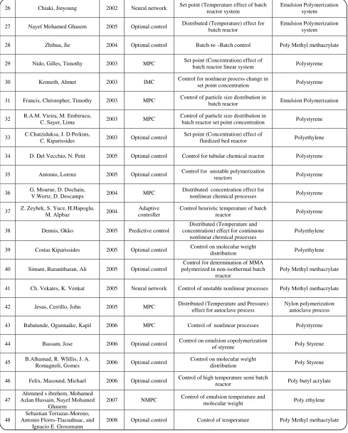
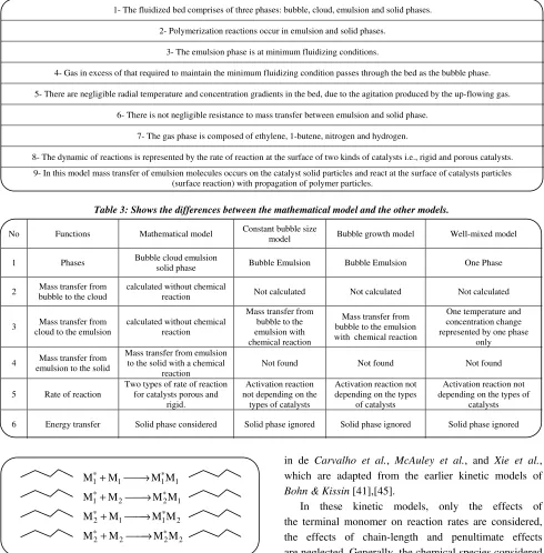
Table 2: List of model assumptions.
1- The fluidized bed comprises of three phases: bubble, cloud, emulsion and solid phases.
2- Polymerization reactions occur in emulsion and solid phases.
3- The emulsion phase is at minimum fluidizing conditions.
4- Gas in excess of that required to maintain the minimum fluidizing condition passes through the bed as the bubble phase.
5- There are negligible radial temperature and concentration gradients in the bed, due to the agitation produced by the up-flowing gas.
6- There is not negligible resistance to mass transfer between emulsion and solid phase.
7- The gas phase is composed of ethylene, 1-butene, nitrogen and hydrogen.
8- The dynamic of reactions is represented by the rate of reaction at the surface of two kinds of catalysts i.e., rigid and porous catalysts.
9- In this model mass transfer of emulsion molecules occurs on the catalyst solid particles and react at the surface of catalysts particles (surface reaction) with propagation of polymer particles.
Table 3: Shows the differences between the mathematical model and the other models.
No Functions Mathematical model Constant bubble size
model Bubble growth model Well-mixed model
1 Phases Bubble cloud emulsion
solid phase Bubble Emulsion Bubble Emulsion One Phase
2 Mass transfer from bubble to the cloud calculated without chemical reaction Not calculated Not calculated Not calculated
3 Mass transfer from
cloud to the emulsion
calculated without chemical reaction
Mass transfer from bubble to the emulsion with chemical reaction
Mass transfer from bubble to the emulsion with chemical reaction
One temperature and concentration change represented by one phase
only
4 Mass transfer from
emulsion to the solid
Mass transfer from emulsion to the solid with a chemical
reaction
Not found Not found Not found
5 Rate of reaction
Two types of rate of reaction for catalysts porous and
rigid.
Activation reaction not depending on the
types of catalysts
Activation reaction not depending on the types
of catalysts
Activation reaction not depending on the types of
catalysts
6 Energy transfer Solid phase considered Solid phase ignored Solid phase ignored Solid phase ignored
Fig. 2: Four plausible polymerization steps
In the simplest case, where only two monomers M1, M2 are involved, the four plausible polymerization steps can be illustrated in Fig. 2 as follows.
The kinetic mechanism of ethylene-butene copolymerization involves a large number of simultaneous and parallel reactions and a myriad of inorganic species. The kinetic mechanism of copolymerization can be found
in de Carvalho et al., McAuley et al., and Xie et al., which are adapted from the earlier kinetic models of
Bohn & Kissin [41],[45].
In these kinetic models, only the effects of the terminal monomer on reaction rates are considered, the effects of chain-length and penultimate effects are neglected. Generally, the chemical species considered in this modified mathematical model are active sites, cocatalyst, live polymers, dead polymers, chain transfer agent, impurities, and poison.
The concentration of these species is denoted by a pair of bracket enclosing the species, the concentration of ethylene, butane, hydrogen, potential active sites, active sites, live polymers, and dead polymers are represented by [M1], [M2], [H2], [P0], [Pn,i] and [Qn] respectively [71],[33],[46],[69].
* *
1 1 1 1
* *
1 2 2 1
* *
2 1 1 2
* *
2 2 2 2
M M M M
M M M M
M M M M
M M M M
+ →
+ →
+ →
When supported catalyst particles are injected into the polymerization reactor, the chemical species take part in a series of complex reactions at the interface between the solid catalyst and the polymer matrix, as follows.
Spontaneous activation: o kn o
P →P (1)
Initiation: kij
o j 1j
P +M →P , J=1, 2 (2)
Propagation:
p i, j
k
nj j n 1, j
P +M →P + (3) i, j 1, 2 , n= =1, 2,...,∞
Chain transfer:
f i, j
k
nj j 1,i n
P +M →P +Q (4) i, j 1 , n= =1, 2,...,∞
Chain transfer to H2:
h i, j
k
nj 2 o n
P +H →P +Q (5) i, j 1, 2 , n= =1, 2,...,∞
The reaction begins by the formation of active sites (1), which is assumed to take place in excess of cocatalyst. This reaction is followed by initiation reactions (2), in which the monomer gases and the active sites are combined to form live polymers. The live polymers then grow according to the propagation reactions (3). Most dead polymers are produced by chain transfers reactions, which can occur in several ways[48], [49]. For simplicity, only chain transfers to monomers (4) and hydrogen (5) are considered in the kinetic modeling. From the kinetic mechanism, the rate expression for each species can be written and the rate expression for the active sites rpο· can be written as follows:
0
p
r = Active site formation - Active site consumption
2
n 0 i
j 0 j
j 1
k [P ] k [P ][M ]
=
− (6)
It is therefore desirable if the kinetics and rate expressions could be manipulated to a simple form. So, the kinetic mechanism outlined in Eq. (1-5) may be viewed as if it is equivalent to the pseudo kinetic mechanism below:
n
k 0
0
P →P (7)
i
k
0 0
P +M→µ (8) p
k
0 M 0
µ + →µ (9)
f
k
0 M P1 0
µ + → + ν (10)
h
k *
2 0 0 0
H + µ →P + ν (11)
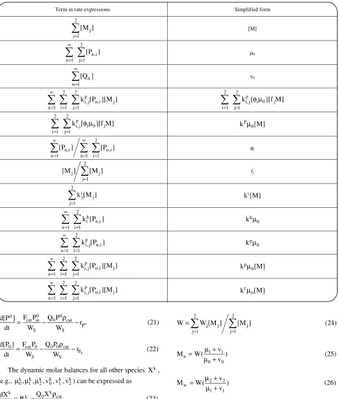
When [M],µo, o are the collective representations of the concentrations of the monomers, live polymer, and the dead polymer. Table 4 gives the simplified form of terms that are found the rate expressions of the species, using method of pseudo kinetic rate constants [64],[65].
For binary copolymerization system, H. Tobita & A. E. Hamielec, 1991, have shown that
p 1 2,1
1 p p
1 2
2,1 1,2
k f
k f k f
φ =
+ (12)
p 1 1,2
2 p p
1 2
2,1 1,2
k f
k f k f
φ =
+ (13)
Therefore the pseudo kinetic constants can be written as follows:
2 2
i i
j j j
j 1 j 1
k k [M ] [M ]
= =
= (14)
2 2
p p
h h
i 2 [i / 2],i i 2 [i / 2],i i
i 1 i 1
k k k − [M ] k − [M ]
= =
= (15)
2 2
p p
h h
j i, j 2 [i / 2],i i 2 [i / 2],i i
i 1 i 1
k k k − [M ] k − [M ]
= =
= (16)
2 2
p p p p
i i
j i, j 2 [i / 2],i 2 [i / 2],i
i 1 i 1
k k k − [M ] k − [M ]
= =
= (17)
2 2
p p
j j
j
j 1 j 1
k k [M ] [M ]
= =
= (18)
2 2
f f
j j j
j 1 j 1
k k [M ] [M ]
= =
= (19)
The dynamic mass balance for the catalyst is as follows:
Accumulation=in by flow - out by flow
cat cat 0 cat cat
s s
dC F Q C
dt W W
ρ
= − (20)
Table 4: Simplified terms in rate expression.
Term in rate expressions Simplified form
2 j j 1 [M ] = [M] 2 n,i n 1 j 1
[P ] ∞ = = µ0 n n 1 [Q ] ∞ = ν0 2 2 p n,i j i, j n 1 i 1 j 1
k [P ][M ]
∞
= = =
2 2
p
i 0 j
i, j i 1 j 1
k [ ][f M]
= =
φ µ
2 2
p
i 0 j
i, j i 1 j 1
k [ ][f M]
= =
φ µ P
0
k µ [M]
2
n,i n,i
n 1 n 1 i 1
[P ] [P ]
∞ ∞ = = = φi 2 j j j 1
[M ] [M ]
= fi 2 i j j j 1
k [M ] = i k [M] 2 h i n,i
n 1 i 1
k [P ] ∞ = = h 0 k µ 2 p n,i i, j n 1 i 1
k [P ] ∞ = = p 0 k µ 2 2 p n,i j i, j n 1 i 1 j 1
k [P ][M ] ∞
= = =
p 0
k µ [M]
2 2
p
n,i j
i, j n 1 i 1 j 1
k [P ][M ] ∞
= = =
f 0
k µ [M]
0
0 0
0
cat in 0 cat
P
S S
F P Q P
d[P ]
r
dt W W
ρ
= − − (21)
0
0 cat 0 0 0 cat
P
S S
d[P ] F P Q P
r
dt W W
ρ
= − − (22)
The dynamic molar balances for all other species Xk,
(e.g., k k k k k k
0, 1, 2, v , v , v0 1 2
µ µ µ ) can be expressed as
k k 0 cat k X S Q X dX R dt W ρ
= − (23)
These leading moments are used in the calculation of weight average molecular weight Mw and number average molecular weight Mn.
2 2
j j j
j 1 j 1
W W [M ] [M ]
= =
= (24)
1 1
n
0 0
v
M W( )
v µ + =
µ + (25)
2 2
w
1 1
v
M W( )
v µ + =
µ + (26)
Where Wj is the molecular weight of the monomer / comonomer.
In this study the polymerization with less porous catalyst particles tends to take place first only at the exit of a particle due to the emulsion molecules diffusion and chemical reaction happening at the exit surface of catalyst particle then emulsion particles can easily diffuse into the porous of the catalyst particles[50],[51],[59].
The reactant adsorption as represented by Eq. (27), the surface reaction as represented by Eq. (28), and the product desorption as represented by Eq. (29) to produce the overall reaction of equation represented by Eq. (30) as, seen below;
A AS
C + ↔S C Reactant adsorption (27)
AS BS
C →C Surface reaction (28)
BS B
C →C Product desorption (29)
A B
C →C Overall reaction (30) Rate of surface reaction is the controlled reaction, where the rate of adsorption and the rate of desorption is limited as, seen below: Eqs. (31) and (33) will be reduced to the following:
Rate of reaction adsorption
AD A A V AS A
r =K (P C −C / K ) (31)
Rate of reaction in the surface:
S S AS BS S
r =K (C −C / K ) (32)
Rate of desorption:
D D BS B D
r =K (C −C / K ) (33)
The overall reaction must be controlled by the rate of reaction surface so, the rate of adsorption and desorption must be equal zero so as to simplify the solution. Hence,
AD A A V AS A
r = =0 K (P C −C / K ) (34)
A V AS A
P C =C / K
AS A V A
C =P C K (35)
D D BS B D
r = =0 K (C −C / K ) (36)
BS B D
C =C / K (37)
T V AS BS
C =C +C +C (38)
T V A A B D
C =C (1 P K ) C / K+ + (39)
A A V
C =P C
A A T B D A A
C =P (C −C / K ) /(1 P K )+
From the kinetic mechanism, the rate expression for each species can be written and the rate expression for the active sites rP0 can be written as follows;
0
P
r =Active site formation-Active site consumption (40)
2
n O i
i A
1
K [P ] K C
= −
2
n O i
i A T B D A A
1
K [P ] K P (C C / K ) /(1 P K )
= − − +
So, the pseudo kinetic constants and rate of reactions will be change according to the kind of catalyst as in Eq. (40) so these effects will affect on the live and dead moment’s equations in calculation of temperature, concentration of emulsion phase and molecular weight.
The estimation of the reactor model parameters are given
in [1]. From Fig.1, it can be seen
that the polymerization process in the fluidized bed reactor occurs in three basic steps as, follows:
1. Bubble phase to cloud phase (Step 1). 2. Cloud phase to emulsion phase (Step 2).
3. Mass transfer with chemical reaction from emulsion phase to the catalyst phase and propagation in size and molecular weight of the polyethylene particle (Step 3).
The mass and energy balance equations pertinent to each of these steps are described below where the meaning of all symbols can be found in the nomenclature section.
These steps are giving us a clear picture about operation of polymerization system as see in Fig.1. Many researchers are ignored the relationship between bubble phase and cloud phase; and between emulsion phase and solid phase. The solid phase factor is very important and has big effects on polymerization process because when increased the mass fraction of the catalyst phase in a very small a mounts will find a big change will happen in the results of emulsion temperature and concentration [57],[58].
So, in this study will explain in details the three steps with derivative modified mathematical model and all the calculations.
Bubble Phase to Cloud Phase of Ethylene (Step 1)
This step represents the first operation step in fluidized bed. Mass transfer from bubble phase to the cloud phase without chemical reaction happens in this step and this assumption is not the same like Choi & Ray,
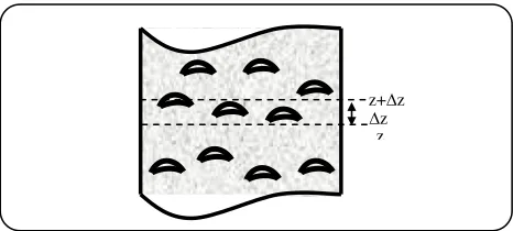
Fig. 3: Section of a bubbling fluidized bed.
assumption different from D. Kunii & O. Levenspiel
assumption because no chemical reaction that was happened in this step[52],[53].
Material balances will be written over an incremental height ∆z for substance A in each of the three phases (bubble, cloud, and emulsion) as seen in Fig. 3.
Mass balance on the bubble phase
The amount of A entering at is the bubble phase by flow,
b c Ab
(u A C )δ =[molar flowrate enter the filled with bubble]× [fraction of bed occupied by bubble]
A similar expression can be written for the amount of a leaving in the bubble phase in flow at z+∆z:
In by flow = out by flow + out by mass transport Dividing by Ac∆zδ and taking the limit as ∆ →z 0 yields
b c AB x b c AB x x
(u A C )( )δ −(u A C )( )δ +∆ −
bc AB AC c
K (C −C )A ∆ δ =Z 0
A balance on A in the bubble phase for steady-state operation in section ∆z is given by
(
)
Ab
b bc Ab Ac
dC
u K C C
dZ = − − (41)
Ab Ab0
At Z=0, C =C
Superficial velocity has big effect on monomer temperature because it effects on minimum fluidization velocity, bubble velocity, inlet gas volumetric flow rate to the bubble phase and heat transfer coefficient that leads to direct proportional effects on monomer temperature.
Energy balance on the bubble phase
For energy system balance in two states in bubble phase will find the variation of bubble temperature with the height of fluidized bed is the same behavior like Choi &
Ray; McAuley et al. and Hatzantonis assumptions [67],[70].
(
)
bc(
)
Ab b ref c b
b pg H d
C T T T T
dZ − = u C − (42)
Cloud phase to emulsion phase (Step 2)
This step represents the second operation step in fluidized bed. Mass transfer from cloud phase to the emulsion phase without chemical reaction happens in this step as seen in Fig. 4 and this assumption is not the same like Choi & Ray; McAuley et al. and Hatzantonis
assumptions because these assumptions not have mass transfer from bubble phase to the cloud phase[72],[73].
Mass balance on the cloud phase
In the material balance on the clouds and wakes in section ∆z, it is easiest to base all terms on the bubble volume. The material balance for the clouds and wakes is Accumulation=in by flow - out by flow + in by mass transport - out by mass transport + generation i.e.
c c
Ac z Ac z z
u u
0 ( C ) ( C )
z ↓ z ↓ +∆
= − +
∆ ∆
(
)
(
)
bc Ab Ac ce Ac Ae
K C −C −K C −C +0
c
u (cloud velocity)=
c w
b
bed
V (volume of cloud) V (volume of weak) u
V (volume of bed)
+ ×
Using the Kunii-Levenspiel model, the fraction of the bed occupied by the bubbles and wakes can be estimated by material balances on the solid particles and the gas flows. The parameter δ is the fraction of the total bed occupied by the part of the bubbles that does not include the wake, and α is the volume of wake per volume of bubble. The bed fraction in the wakes is therefore αδ. The bed fraction in the emulsion phase (which includes the clouds) is (1 - δ - αδ).
c mf mf
b b mf mf
V 3(u / )
V u (u / )
ε =
− ε
So, the mass transfer equation from cloud to the emulsion is represented by Eq. (43).
Ac
mf mf
b
b mf mf
dC
3(u / )
u [ ]
u (u / ) dz
ε
δ + α =
− ε (43)
(
)
(
)
bc Ab Ac ce Ac Ae
K C −C −K C −C
z z+ z
Fig. 4: Shows the mass transfer of emulsion molecules to the catalyst particles Micrography of Ziegler-Natta Catalyst by scanning electron microscope (Wolf et al., 2005).
Energy balance on the cloud phase
For energy balance pass in two states from cloud phase to emulsion phase the variation of cloud temperature with the height of fluidized bed is the same as Choi & Ray; McAuley et al. and Hatzantonis
assumptions i.e.
(
)
ce(
)
Ac c ref e c
c pg H d
C T T T T
dZ − =u C − (44)
Mass transfer with chemical reaction from emulsion phase to the catalyst phase and propagation in a size of polyethylene particle (Step 3)
This step represents the third operation step in fluidized bed. Mass transfer from emulsion phase to the catalyst phase with chemical reaction happens in this step as seen in Fig. 4 .and this assumption is not the same
like Choi & Ray; McAuleyet al. and Hatzantonis. Mass balance on the emulsion phase
In the material balance on the clouds and wakes in section z, it is easiest to base all terms on the bubble volume. The material balance for the clouds and wakes is:
Accumulation=in by flow - out by flow + in by mass transport - out by mass transport + generation i.e.
Ae
1 mf
dC A H
dt
ε = (45)
[
]
E,C 1 Aece Ac Ae 1 mf a s
D A dC
K C C A H r W
dr −
− ε + +
To simplify the solution
E,C 1 Ae
AO Ae Ae mf
D A dC
G1(C C ) Q0C
dr −
= − − ε (46)
Where
DE,C Diffusivity of emulsion particles towards catalysts particles (m2/sec)
So the Eq. (45) will be:
[
]
Ae
1 mf ce Ac Ae 1 mf
dC
A H K C C A H
dt
ε = − ε + (47)
Ao Ae o Ae mf a s
G1(C −C ) Q C− ε +r W
Energy balance on the emulsion phase
phase to the solid phase. So, will find the variation of emulsion temperature with the time is not the same behavior as of Choi & Ray; McAuley et al. and
Hatzantonis assumptions and is given by.
(
)
{
}
e1 mf s ps mf me pg
dT
A H 1 C C C
dt
− ε ρ + ε + (48)
(
)
me(
)
1 e ref mf pg me pg e f
dC
A H T T C GC C T T
dt
− ε = − − +
(
)
(
)
(
)
B be b e r p 0 mf me pg
A H T −T dz+ −∆H R −Q ε C C
(
Te−Tfs)
−Q0 mfε CmeCpg(
Te−Tf)
−(
*)
(
)
w e w
DH 1 h T T
π − δ −
Nonlinear model predictive control
Motivated by the advancements of computer technologies and control analysis techniques, more sophisticated control system design procedures have appeared during the past two decades which includes the Nonlinear Model Predicative Controller (NMPC) as mentioned in the previous section. Model Predictive Control (MPC) refers to a class of algorithms that compute a sequence of manipulated variable adjustments in order to optimise the future behaviour of a plant. Originally developed to meet the specialized control needs of power plants and petroleum refineries, MPC technology can now be found in a wide variety of application areas including chemical production, food processing, automotive, aerospace, metallurgy, pulp and paper industries (O. Abel et al., 2001)
The application of MPC for many industrial processes has shown great accomplishments in the past years and it is gaining popularity as an efficient and reliable control algorithm due to its many important features. This feature include its ability to deal with uncertain ties robust to change control objectives, ability to handle process time delays, can handle interacting variables well, in multivariable systems and eliminates stability problems created by constraints[29],[23],[66].
Neural Network Model Predictive Control technique (NNMPC)
However the strength of the NMPC method depends on the accuracy of the nonlinear model incorporated into the model predictive framework. This is normally difficult in many cases dealing with nonlinear system especially this highly nonlinear polymerization system,
the details of the mathematical model of which can be seen in previous section[3],[7].
However, due to the versatile nature of the Artificial Neural Network (ANN) models for nonlinear systems, it is an excellent candidate to use for modelling the polymerization system and incorporate within the model predictive framework and this is the approach taken to control this system in what is called neural network based model predictive control study[9],[28].
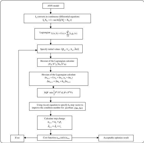
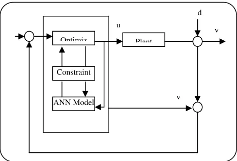
Fig. 5 shows the neural network based MPC scheme. The non-linear optimizer in the MPC is used to select the manipulated variable that minimizes a cost function, which is quadratic in the set point/process output error. To do so, the non-linear optimizer uses the ANN process model to predict the possible future responses of the process to calculate the manipulated variable sequences. By using the ANN model to predict multi-step ahead, the control scheme can anticipate the process trajectory and compensate for measured disturbances before their impact on the process output is detected[14],[47].
The general philosophy of the neural network MPC is identical to that of the standard MPC method. The controller determines a set of future manipulated variable moves that minimize a cost function over a prediction horizon, subject to input and output constraints. The cost function usually includes the sum of squares of the errors between the predicted outputs and the set point values evaluated over the prediction horizon, and commonly also includes a term which penalizes the rate of change of the manipulated variable. For such a cost function, the MPC problem can be posed as follows,
i P2
2
i P1
min u(t) J (y(t i) r(t i)) =
=
= + − + + (49)
i C
2
i 1
(u(t i 1) u(t i 2)) =
=
λ + − − + −
where…
u(t+ =i) u(t+ −C 1), i>=C
min max
du ≤u(t)≤u
Where J is the cost function to be minimized, P1 to P2 define the prediction horizon, C is the control horizon,
(
)
Fig. 5: Represents all optimize control steps.
corrections should be made to the model output to account for process/model mismatch and unmeasured disturbances Fine T.L. & Smith M., and this can be done with an additive disturbance, e (t) as [14],[47]
'
ˆ
y(t+ =i) y(t) e (t)+ (50) Where y t
(
+i)
is the i-step ahead ANN model prediction. A simple approach, which was adopted here,is to use the process/model mismatch to estimate this disturbance, i.e.
' ˆ
e (t)=y(t)−y(t) (51)
Introduction of the modified set point, r (t)' gives
' '
r (t+ =i) r(t+ −i) e (t) (52)
Combining Eqs. (50) to (52) in Eq. (49) gives…
ANN model
Ig converts to continuous differential equations
o
k k k k
I X = −1 sec h{ (Xξ −X )}
Specify initial values (ρo, v , x , o)o o λ
Lagrangian m
f f
i 1
L(x, ) f (x) g (x)
=
λ = + λ
Hessian of the Lagrangian calculate
2 2
( y,∇ ∇y, u,∇ ∇u)
Hessian of the Lagrangian calculate
k 1 k k k k
x+ f (x x , u u )
∆ = + ∆ + ∆
k 1 k k k 1
u+ u k x +
∆ = ∆ + ∆
T 2 T
1
SQP min P ( xL)P P x
2 ∇ + ∇
Using riccati equation to specify kk step vactor to
improve the condition number for jacobian (∆ ∆u, x)
Calculate step change
1
1
k k o
k k o
u u
v
ρ λ λ
+ +
= +
= +
Cost function umin u(t) umax Acceptable optimize result
i P2
' 2
i P1
ˆ
min u(t) J Q (y(t i) r (t i)) =
=
= + − + + (53)
i C
2
i 1
(u(t i 1) u(t i 2)) =
=
λ + − − + −
In this study y (t) represents the emulsion temperature and molecular weight which are the controlled variable and the while variable u (t) represents superficial velocity and catalyst flow rate. The optimization problem outlined by Eq. (53) is solved using the Sequential Quadratic Programming (SQP) algorithm[155],[21].
Sequential Quadratic Programming (SQP)
The SQP method allows us to mimic Newton’s method for constrained optimization. At each iteration, a method similar to Newton’s method is used to generate a quadratic programming sub problem whose answer is used to determine a search direction for the solution[77].
Since the iterative optimization algorithm employs an analytical gradient method, each term in the control model should be everywhere differentiable. Therefore, the discontinuous binary variable Ik in the objective function needs to be converted into a continuously differentiable function[20],[79]. In this work, Ik is approximated by the following smooth function:
o
k k k k
I X = −1 sec h{ (Xξ −X )} (54)
and
o
k k k k
I X = −1 (1/(1/ e−ξ(X −X ))) (55)
Where ξ is a suitably large number. It tends to rapidly converge from zero to one, as o
k k
(X −X ) goes from zero to a large value. Therefore, a suitable large n ensures that it is not only binary but also differentiable. With this approach, Ik can be converted to a continuously differentiable function at the price of some inaccuracy by approximation. A number of other smooth approximation functions are also available from Biegler, 1998 [44],[60],78] .
The computational efficiency associated with solving an optimization problem is often the key concern in the online implementation of MPC methods. However, the conventional MPC methods experience an extremely large computational burden for large-scale manufacturing
processes. The computational burden rapidly increases as the problem size expands. Therefore, to improve the computational efficiency in the on-line optimization, it is necessary to reduce the dimensionality of the optimization problem[16],[61]. For this purpose, we transform the controllable and fixed variables into reduced score variables in the Pulsated prediction model and then optimize for the score variables. A decision variables, t1; . . . ; tA., controllable and fixed variables are expressed by
k 1 1,k A A,k
X =t p + − − − − +t p , k= − − −1, , c (56) Where pA,k is parameters estimation of element pA at each k value.
The objective of optimization is to minimize (or maximize) a function of one or more parameters as in Fig. 5. A set of equality and/or inequality constraints that are also functions of the parameter set, and which confine the parameter values to specified regions of the search space, may also be imposed as part of the optimization problem[22],[75]. A minimization problem may be stated more formally in the following mathematical format: minimize F(x), subject to: g(x) and h(x)>=0,
where x is a real-valued vector of variable parameters,F(x) is a scalar-valued cost function, and g(x) and h(x) are vectors of constraint functions. The solution to the general optimization problem is obtained by Lagrange Multiplier analysis[6],[18]. The Lagrangian for the standard optimization problem may be written as
T T
L(x, , )λ µ =F(x)− λ g(x)− µ h(x) (57)
Where and are Lagrange multiplier vectors. The following Kuhn-Tucker necessary (Baker et al, 2002 and
Fine, 1999) conditions for a local minimum may be applied to gain potential solutions to this problem as;
T T
i i i i
F(x) g(x) h(x)
L
x x x x
∂ ∂ ∂
∂ = − λ − µ
∂ ∂ ∂ ∂ (58)
Th(x) 0
µ = µ ≥j 0
may be applied to find an approximation to the solution of (57). The SQP method produces iterative estimates of the optimal parameter values and the Lagrange multipliers. As the numerical algorithm converges, these iterative estimates approach the optimal parameter values and Lagrange multipliers that would result from the analytical method Eq. (58), if it were applied. The primary computational components of a sequential quadratic program are responsible for the formation of an iterative locally quadratic approximation to the Lagrangian function, and a sufficient decrease line search of an augmented Lagrangian merit function[19],[20],[76]. An iterative quadratic approximation to the Lagrangian is given by,
q k k k q k 1 k 1 k 1
L (x ,λ µ, )=L (x −,λ −,µ −)+ (59)
T T T T
k q k 1 k 1 k 1 k k k
1
d g(x) h(x)L (x , , ) d B d
2
− − −
∇λ − µ λ µ +
Where ∇ is the gradient operator (with respect to x ), and
x k k 1
d =x −x − (60)
And x and xk k 1− are the values of the parameter vector x at the current iteration and the previous iteration, respectively. The second-order partial derivative, or Hessian, approximation matrix, BK in Eq. (61), is generated by variable metric update equations[25]. The update that is typically applied is the Broyden-Fletcher-Goldfarb- Shanno (BFGS) update which was modified by
M.S. Bazaraa et al., 1993 as:
T T
k 1
k k 1 T T
k 1
B ss
B B
sB s s
− −
−
ηη
= − +
η (61)
Where
k 1 k 2
s=x − −x − (62)
k 1
(1 )B −s
η = θω − − θ
q k 1 k 1 k 1 q k 1 k 1 k 1
L (x −, − , − ) L (x −, −, −)
ω = ∇ λ µ − ∇ λ µ
and
T T
k 1
T k 1
1if s 0.25s B s
0.8
s B s
−
−
ω
θ = (63)
The quadratic approximation to the Lagrangian function is solved for the direction, dk, in parameter
space that points in a minimizing direction of the quadratic. The variable metric matrix, Bk, must remain positive definite to ensure a bounded solution for the search direction, dk . In practice, a positive definite Bk is maintained by the Levenberg-Marquardt method or by storing the variable metric updates in Cholesky
decomposed form (P.E. Gill et al., 1981). The positive definite state of Bk enables from Eq. (61) to be solved as a minimization problem. In a numerical setting, the quadratic approximation to the Lagrangian may be recast, through primal-dual relationships (P.E. Gill et al., 1981), into the following quadratic sub problem with linearized constraints:
subject to:
k
T T
d k 1 k k 1 k k k
min F(x −) d+ ∇F(x − ) d B d+ (64)
T
k 1 k k 1
subject to :g(x −) d+ ∇g(x − )=0
T
k 1 k k 1
h(x −) d+ ∇h(x −)≥0
The maintenance of a positive definite Bk ensures that the local approximation given in Eq. (61) can be readily solved for the search direction, dk , through standard convex quadratic programming methods (Evanghelos Zafiriou and Hung-Wen Chiou, 1992)[24],[43]. In practice, other numerical techniques may be applied to prevent the linearized constraint approximations from completely closing off the feasible region Fine T.L., 1999 and SmithM., 1996. An active sets strategy (Evanghelos Zafiriou & Hung-Wen Chiou, 1992) is also employed so that only the inequality constraints that are satisfied to within some small tolerance of an equality are included in the quadratic model, thereby reducing the overall computational effort[26],[32].
Following solution of the quadratic subproblem, a one-dimensional line search along the minimizing direction, dk, is conducted. Another class of approximations to the Lagrangian (augmented Lagrangian merit functions) is typically used for this phase of the analysis. The centralize NNMPC techniques is used in our controller because it is control each parameters inside the system as shown in Fig. 6. The following merit Eq. (64) was used for this analysis as:
T T
k k k k k k
W(x ,λ µ, )=F(x )+ λ g(x)+ µ h(x) (65)
Fig. 6: The general structure of a nonlinear MPC.
decrease in the value of Eq. (65) is found. The candidate points are generated from the line search update Eqs. (65) and (66).
k k 1 k
x− =x − + αd (66)
Neural Network Modeling
Before implementing the neural network based MPC a sufficiently accurate Artificial Neural Network (ANN) model of the polymerization system needs to be obtained. The steps used to obtain these models are outlined in the following section with some background of neural network itself[27],[36].
Basically, the ANNs are numerical structures inspired by the learning process in the human brain. They are constructed and used as alternative mathematical tools to solve a diversity of problems in the fields of system identification, forecasting, pattern recognition, classification, financial systems and many others (Huang & Mujumdar, 1993; Joaquim & Dente, 1997, Shaw et al., 1997; Baker & Richards, 2002). The interest in ANN as a mathematical modeling tool resulted in the consolidation of its theoretical background and the development of its underlying learning and optimization algorithms (Ang D.D. et al 1998; Huang, B et al,1993 ;
Joaquim, A et al , 1997 and Shaw,et al ,1997).
Modeling and simulation of chemical processes is one of those research areas of interest that made use of ANN modeling techniques. The implementation of mechanistic models that rely on fundamental material and energy balances as well as empirical correlations involves a great deal of mathematical difficulties and in many instances lacks accuracy. Neural network-based modeling can be
used confidently as a substitute for such situations. This is due to the favorable features entailed in their use. Among these features are; simplicity, fault and noise tolerance, robustness and ability for modelling nonlinear systems. The ANNs can be categorized in terms of its topology such as the multi-layer Feed Forward Neural Networks (FFNN), FeedBack Neural Networks (FBNN), Recurrent Neural Networks (RNN) and self-organized networks[34],[38]. In addition, they can be further categorized in terms of application, connection type and learning methods. FFNNs are the most commonly used type for function approximation. In this topology, the network is composed of one input layer, one output layer and a minimum of one hidden layer. The term feed forward describes the way in which the output of the FFNN is calculated from its input layer-by-layer throughout the network. In this case, the connections between network neurons do not form cycles. No matter how complex the network is, its building block utilizes a simple structure using the neurons. It performs a weighted sum of its inputs and calculates an output using certain predefined activation functions. Activation functions for the hidden units are needed to introduce the nonlinearity into the network. The Sigmoidal functions, such as logistic and tanh, and the Gaussian function, are the most common choices for the activation functions. The number of neurons and the way in which the neurons are interconnected defines the neural system architecture. The network is fed with a set of input-output pairs and trained to reproduce the outputs. Adjusting the neurons weights using an optimization algorithm to minimize the quadratic error between observed data and computed outputs do the training. A good reference on the FFNN and their applications is given by Fine, 1999.
Input-target training data are usually pretreated in order to improve the numerical condition for the optimization problem and for better behavior of the training process. Thus, the data are normally divided into three subsets; training, validation and testing subsets. The training subset data are used to accomplish the network learning and fit the network weights by minimizing an appropriate error function. It refers to the method for computing the gradient of the error function with respect to the weights for a feed forward network. Evaluating the error function using the validation subset data, independently, then compares the performance of the network. The testing subset data are then used to measure
Plant
ANN Model Constraint
Optimiz
y d u
Fig. 7: Three layer feed forward neural network
the generalization of the network (i.e. how accurately the network predicts targets for inputs that are not in the training set). Improperly trained neural networks may suffer from either under fitting or over fitting. The former describes the condition when a network that is not sufficiently complex fails to fully detect the signal in a complicated data set. On the other hand, the latter condition occurs when a network that is too complex may fit the noise, in addition to the exiting signal (Smith, 1996).
Selecting network structure is a crucial step in the overall design of NNs. The structure must be optimized to reduce computer processing, achieve good performance and avoid over fitting. Experience in using ANN for function approximation revealed that any nonlinear function can be approximated by a three layer ANN structure. The selection of the best number of hidden units depends on many factors. The size of the training set, amount of noise in the targets, complexity of the sought function to be modeled, type of activation functions used and the training algorithm all have interacting effects on the sizes of the hidden layers. Details of training a neural network can be found in
M.S. Bazaraa et al., 1993. The finally trained ANNs represent the general relations linking ANN inputs to its output for the modified mathematical model of the fluidized bed for the gas phase olefin polymerization reactor.
Neural Network modeling of Polymerization System The data used for training the neural network model was generated from the non linear model of the system (hammed et al.,2008. Step tests data were generated in simulation for the model with change in inputs values for superficial velocity and catalyst flow rate as shown in Fig. (11) and (12).
The inputs corresponding ranges for all gases mole fraction concentrations were form with other superficial velocity were from (0.1 to o.75) and for temperature input range from (300-395 K). The selected ranges cover the whole spectrum of model system including of flooding conditions and both outlet emulsion temperature and molecular weight. Data sets were divided into three subsets; training, validation and testing.
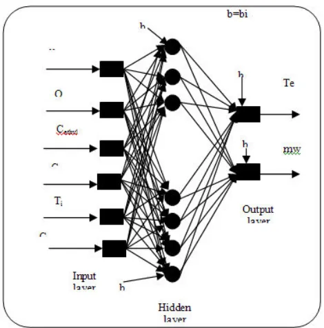
The neural network structure was selected based on testing different network configurations that vary in terms of structure and simulation parameters. The criterion for network structure selection is based on its simplicity, performance, and accuracy of model prediction. The finally selected network contained 1 hidden layer with 8 neurons. The activation function used in the hidden layer is the tanh function because it is more suitable for the highly non linear system, while the output layer contains linear neurons. The inputs and outputs to the network are as shown in Fig. 7.
Fig. 7 six input with the time -two outputs data sets were generated by introducing random steps in the manipulated variables at a sampling time 3h and collecting the outputs emulsion temperature Te and molecular weight MW.
So, we can specify the inputs as (uo(t,t-1,...,t-n+1)),Qc(t,t-1,...,t-n+1),Cethylene (t,t-1,...,t-n+1), Cbutene (t, t-1,...,t-n+1), Tin (t, t-1,...,t-n+1)and Chydrogen (t, n+1)) and outputs (Te (t, t-1,...,t-m+1) and MW (t,) t-1,...,t-t-1,...,t-m+1).The neural network shown in Figs. 4.4 to 4.6 is in the process of being trained using a feed forward neural net work.
Fig. 8: Input-output training set for molecular weight ANN predictions.
Fig. 10: Analyses for validation data
In "Reaction Kinetics" section, it has been shown that the fluidized bed polyethylene process is highly nonlinear, especially with excitations in the superficial gas velocity and that the effect of nonlinearity is more pronounced on emulsion temperature and molecular weight than the catalyst flow rate but both these inputs have big effect on the system. The central control system for NMPC can be controlled by each variables input inside the system. This system is affected by four disturbances, namely concentration of ethylene (Cethylene), concentration of butane (Cbutene), concentration of hydrogen (Chydrogen) and temperature input Tin. This configuration is adopted in this study.
In order to facilitate the use of the control algorithms to be studied, a neural network model of the fluidize process under consideration is constructed. This is achieved by generation a set of input-output network training data using the developed mechanistic model. Used two networks for the two set points emulsion temperature and molecular weight. The Levenberg-Marquardt Back Propagation (LMBP) optimization algorithm was used for network training. This algorithm gives good performance with an average error for
the two networks (uo-Te) and (Qc-MW) was 1×10⁻⁸. The achieved networks then were validated and tested using the data subsets previously generated from the model. A comparison of both modeled and network-predicted outputs for both phases is shown in the form of the error profiles in Figs. 8, 9, and 10. These Figures indicate low errors even under severe process excitations.
SQP approach utilizing the Quasi-Newton method with a conjugate gradient algorithm was used for the nonlinear constrained optimization in NMPC as Has been previously explained in "SQP" section 4.2 and Fig. 6.
Simulation and Results
The neural network models obtained as for training in the previous section were utilized in model predictive Schemes as described in previous section. Simulation studies including set point tracking and disturbance rejection studies such as changes in hydrogen, butene, ethylene concentrations, inlet temperature, superficial velocity and catalyst flow rate were done in this work.
For the case of constrained control, the MPC was able to drive the system dynamics to the desired values effectively without violating the limitations assigned for
0 10 20
0.4 0.5 0.6
0.7 Input
0 10 20
372 374 376 378 380
Plant Output
0 10 20
-4 -2 0 2 4
6 x 10 -3 Error
time (s)
0 10 20
372 374 376 378 380
NN Output
Table 5: Dynamic response characteristics for a set point of emulsion temperature.
Tuning Method LOOP Rise time (min) Overshoot Settling time IAE (min)
MPC
Uo-Te 1.23 - 1.255 0.013
Qc-MW 1.35 1.435 0.054
PID
Uo-Te 1.7 - 1.555 2.09
Qc-MW 1.86 - 1.89 2.34
Table 6: Integrated absolute error for set point and disturbance rejection of the emulsion temperature closed loop using the NN-MPC as compared to the PID controller.
Controller Set point
IAE
Disturbance in hydrogen concentration IAE
Disturbance in ethylene concentration IAE
Disturbance in butane concentration IAE
Disturbance in inlet temperature IAE
MPC 0.045 0.0087 0.0106 0.096 0.0128
PID 0.15 0.091 0.109 0.103 0.130
Table 7: Integrated absolute error for set point and disturbance rejection of the molecular weight closed loop using the NN-MPC as compared to the PID controller.
Controller Set point
IAE
Disturbance in hydrogen concentration IAE
Disturbance in ethylene concentration IAE
Disturbance in butane concentration IAE
Disturbance in inlet temperature IAE
MPC 0.1926 0.383 0.2788 0.4382 0.2042
PID 2.255 3.056 2.386 3.755 2.401
Fig. 11: MPC controller response for set point tracking study of superficial gas velocity on set point.
the manipulated variables. Of course there were some little differences between the two controllers in terms of set point tracking time and damping of response, but in terms of control criteria, the constrained case was acceptable and doesn’t have much deviation from the unconstrained one. The characteristics of the dynamic responses are calculated and given in Table 5. The missing values in the table indicate no value or an inapplicable measure.
Fig. 12: MPC controller for set point tracking study of catalyst flow rate on set point.
The Integral Absolute Errors (IAE) of the process responses are shown in Tables 6 and 7.
From the response characteristics of the different tuning algorithms the following can be noticed:
Effects of disturbances on the two outputs are shown in Tables 6 and 7 a good idea about performance of MPC controller.
Figs. 11 and 12 show the neural-network based
MPC Set point
Time (min)
0 2 4 6 8 10
369 370 371 372 373 374 375 376
MPC Set point
Time (min)
0 2 4 6 8 10
M
ol
ec
u
lar
w
ei
g
h
t
k
g/
k
m
ol
Fig. 13: MPC controller for disturbance hydrogen concentration on set point.
Fig. 14: MPC controller for disturbance of butene concentration disturbance on set point.
Fig. 15: MPC controller for disturbance of ethylene concentration on set point
Set point NMPC PID
Time (min)
0 2 4 6 8 10
k g/ k m ol 0 2e+4 4e+4 6e+4 8e+4 1e+5 Set point NMP PID Time (min)
0 2 4 6 8 10
E m u ls ion t em p er at u re °k 0 100 200 300 400 500 600 700 Set point NMPC PID Time (min)
0 2 4 6 8 10
E m u ls ion t em p er at u re °k 0 100 200 300 400 500 600 700 Set point NMPC PID Time (min)
0 2 4 6 8 10
M ol ec u lar w ei g h t k g/ k m ol 0 2e+4 4e+4 6e+4 8e+4 1e+5 Set point NMPC PID Time (min)
0 2 4 6 8 10
E m u ls ion t em p er at u re °k 0 100 200 300 400 500 600 700 Set point NMPC PID Time (min)
0 2 4 6 8 10
Fig. 16: MPC controller for disturbance of inlet temperature on set point.
Fig. 17: Response for set point tracking studies - MPC comparison with PID controllers for superficial velocity rejection study.
predictive controller performance for set point tracking without any oscillations in both cases. The results show that a fast rise time was achieved, with a very small overshoot for both loops.
The disturbances introduced are changes in the initial hydrogen, butene, ethylene concentrations and inlet temperature respectively shown in Figs. 13 to 16 the behavior of MPC is very active and smooth without any oscillations. From Figs. 13 to 16 PID and MPC controllers for disturbance of hydrogen, butene, ethylene concentrations and inlet temperature respectively rejection study on set point show that PID controller is characterized with slightly longer settling times control with a digressive action oscillations before achieving the set point with a higher overshoots compare to MPC as shown in Fig. 17.
From these results it can be inferred that the behavior of comparison of PID and MPC controllers for set point shown in Fig. 17 PID controller is characterized with slightly longer settling times control action with oscillations before achieving the set point with a higher overshoots compare to MPC.
CONCLUSIONS
The trained neural network was capable of capturing the fluidized-bed process dynamics with high prediction efficiency and thus can be used in control applications where the process exhibits high nonlinear dynamics such as the fluidized bed process. The performance of the NN-MPC for the set-point tracking and disturbance case was excellent in forcing the process output variables to their
Set point NMPC PID
Time (min)
0 2 4 6 8 10
E
m
u
ls
ion
t
em
p
er
at
u
re
°k
0 100 200 300 400 500 600 700
Set point NMPC PID
Time (min)
0 2 4 6 8 10
M
ol
ec
u
lar
w
ei
g
h
t
k
g/
k
m
ol
0.0 2.0e+4 4.0e+4 6.0e+4 8.0e+4 1.0e+5 1.2e+5
Set point MPC PID
Time (min)
0 2 4 6 8
E
m
u
ls
ion
t
em
p
er
at
u
re
°k
340 350 360 370 380 390 400 410 420
Set point MPC PID
Time (min)
0 2 4 6 8
M
ol
ec
u
lar
w
ei
g
h
t
k
g/
k
m
ol