A Stepped Pyramidal Reward Factor in Genetic Algorithms for Constrained Optimization of Aeroassisted Orbital Maneuvers

A Stepped Pyramidal Reward Factor in Genetic

Algorithms for Constrained Optimization of

Aeroassisted Orbital Maneuvers

Antonio Mazzaracchio

Sapienza University of Rome, Rome, Italy e-mail: [email protected]

Abstract—This paper presents an efficient method of

securing and accelerating the convergence of genetic algorithms for constrained optimization problems. The method is based on the introduction of a particular form of reward factors, which can be considered as the inverse of the classic penalty function. These factors are coefficients that consider the various constraints of the problem when formulating a fitness function. The proposed shape of the reward factor follows a stepped pyramidal function. The efficiency of the method, which is of general applicability, was demonstrated in the context of an optimization problem for an aeroassisted orbital plane change maneuver. The case study demonstrates the rapid convergence of the genetic algorithm obtained by first satisfying the constraints and subsequently maximizing the objective function of the problem.

Index Terms—Aeroassisted orbital maneuver, optimization,

genetic algorithms.

I. INTRODUCTION

The classical methods employed in other applications are also employed for the optimization of orbital transfers. Such methods can be divided into two main categories: direct methods and indirect methods. Direct methods can be used to solve the optimal control problem via the arrangement of the control variables for each iteration to continually reduce the performance index. The control functions and the state equations are frequently parameterized, and the associated nonlinear programming problem can be solved via recourse to an optimization methodology that is based on the gradient method. The literature discussing these previous aspects is vast and includes studies such as that by Herman and Conway [1], who employed the collocation method (an integration method that has been proven to be equivalent to the implicit methods of Runge-Kutta), and a study by Seywald [2], who introduced the concept of “differential inclusion” specifically for trajectory optimization problems. Differential inclusion employs a finitedifference approach to approximate the state variable differentials, whereas direct collocation employs a finite element approach to approximate the temporal trends of these state variables. Instead, indirect methods use the calculus of variations to obtain a set of necessary conditions for a local optimal solution of the objective function1. The resulting two-point

1

The majority of the related literature indifferently refers to the objective function and the fitness function. In this context, the two terms represent two distinct entities, as defined in Section IV.

boundary value problem presents a significant challenge for obtaining a solution due to its sensitivity to the initial value of the co-state variables. Once a solution for the two-point boundary value problem is obtained, the resulting trajectory is generally the optimal trajectory. Casalino et al. [3] applied this indirect method to the case of optimal aeroassisted geostationary Earth orbit (GEO)-low Earth orbit (LEO) transfers. Traditional methods, such as Newton’s method and the gradient method, are mainly local optimization algorithms that are principally capable of searching local optima. Local optima are points where the objective function assumes values that are lower than the values of the surrounding points. The efficiency of these optimizers is strongly linked to the adoption of a suitable initial guess with accurate values of the derivatives of the objective function. In the absence of these features for the initial conditions, the method may not converge or can produce a local minimum solution, which is frequently unacceptable. These fundamental aspects of these methods generally involve an expert level of intervention by the user. To overcome these limitations, global optimization approaches can be employed. These methodologies allow first approximation sub-optimal solutions to be obtained. In this study, a particular type of global optimization is employed: genetic algorithms (GAs).

II. GENETIC ALGORITHMS

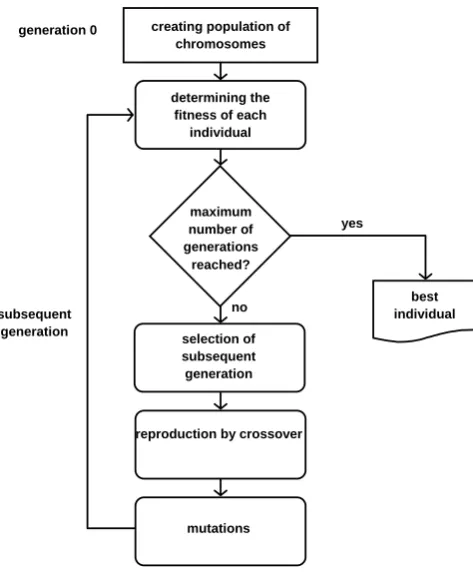
identify the “best individual” who belongs to a population that is subject to an ongoing process aimed at improving a species. As is the case in the biological field, the evolution tends to achieve an improvement instead of an optimum. Thus, a GA “uses” the population at its disposal to generate above-average individuals within the constraints associated with this evolution. Although a GA does not perform a mathematical optimization in the strict sense of the term, these algorithms represent a highly efficient and robust optimization methodology. The GAs developed by Holland [7] are global search optimization methods based on the fundamental principles of Darwinian evolution and include the process of natural selection and genetic mechanisms. Organisms evolve within a time window that involves many generations through changes in their genetic makeup via mating, genetic recombination (crossing over), and mutation. Over time, only organisms with suitable genes perpetuate the species. Figure 1 shows a basic schematic of a generic GA.

creating population of chromosomes

reproduction by crossover

best individual

mutations selection of subsequent generation determining the

fitness of each individual

maximum number of generations

reached? generation 0

subsequent generation

yes

no

Fig. 1. Flowchart of a generic GA.

Generally, a GA employs a representation of individuals using binary strings; however, graphs, lists, or vectors of real numbers are also employed. The type of genetic representation, however, does not change the essence of the algorithm. Individuals or variables are encoded in the search range in such a manner that all information is treated as numeric strings, in which the number of digits (number of genes that constitute the chromosome) is normally an assigned parameter. All individuals (phenotypes), represented by their chromosomes (genotypes), are evaluated by the objective function (or fitness function; refer to Section IV) and assigned a level of fitness, which is an index of the “goodness” of the individual and determines his chance of survival. Several methods are available for

selection; the most common methods are the “roulette wheel” (selection proportional to the fitness), “rank selection”, and “tournament selection”. The iterative process of evolution proceeds by selecting individuals until the stopping criterion is fulfilled. The selected individuals are coupled with each other, and their descendants are generated via genetic mutation and recombination. The new generation consists of these descendants and the parents who satisfy the eligibility requirements to perform another reproductive function. Various types of crossing over operators, such as “one-point”, “multi-point”, and “uniform” crossovers, can be employed. These operators function by swapping genes between the chromosomes of the two parents and allowing the descendants to inherit the characteristics to evolve the solution. The possibility of mutations, whose role, which is not negligible in the overall evolutionary process, is to impose small variations in the population, is less determinant than the crossover operators but should not be disregarded when exploring the search space. Although the progression caused by mutations is frequently slow compared with the progression of crossovers, mutations represent a critical method for obtaining an expanded search space. Mutations also prevent correlation problems within the population to ensure the fundamental diversity required by the crossover process.

III. IMPLEMENTED GA

real field. The encoding requires the specification by the user of the number of genes to maintain. The adopted GA refers to a mixed one-point/two-point crossover operator. The crossover is conditioned to a probability of success but may not be successful. Similarly, the mutation, which may involve any gene, is also subjected to a probability of occurrence, which is dependent on the selected mutation mode. These two probabilities are parameters that can be specified by the user. Although the selected reproduction plan provides for the complete replacement of the previous generation by the new generation (“full generational replacement”), other less dynamic types of generational plans (“steady state replace random” and “steady state replace worst”) can be selected. The user is also given the option to use elitism to retain the individual with the highest fitness from the previous generation in the new generation. This precaution is important because it safeguards against the possibility of removing the best individual in the population via the reproduction-mutation process, thus producing a deceleration of the evolutionary process. The option of dynamically adjusting the probability of mutation reduces the danger of prematurely cancelling robust solutions. To obviate these cases, the probability of mutation is linked to the level of convergence of the solution: the higher the level of convergence, the less likely a mutation will occur.

IV. FITNESS FUNCTION,OBJECTIVE FUNCTION, AND

CONSTRAINTS

As previously mentioned, the objective function defines a different quantity than does the fitness function in the context of this study. In this paper, the fitness function is defined as the sum of the objective function, which is the quantity to be maximized in the analyzed problem, and the contributions of various reward factors, one for each considered constraint. The adoption of this particular scheme in a maximization problem enables a simpler manipulation of the constraints compared with the classical treatment using a penalty function [10]. Using this method, the various reward factors are directly summable to the objective function. The form taken by the reward factor

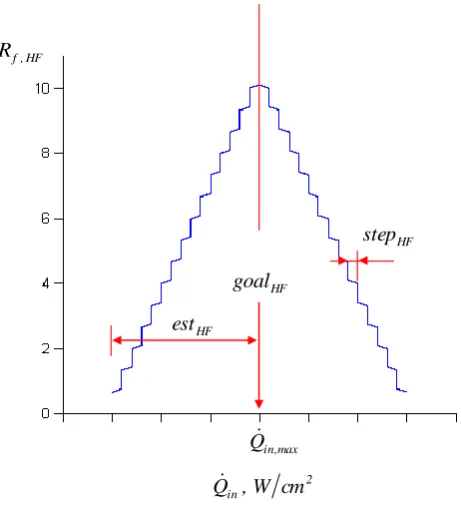
j , f

R , where the index j represents the different considered constraints, is a particular stepped pyramidal function, as shown in the example presented in Figure 2. The function assumes a value of zero outside of the range of definition, i.e., outside of the base of the pyramid, which is bordered by the semi-extension est_j around the imposed value for the

constraint goal_j. Thus, the range of definition will be

[goal_jest_j]. This range is divided into subintervals

(steps); the width of each step is equivalent to step_j and is distinguished by a “level of compliance”, or inversely defined by a “level of violation”, of the constraint. The value assigned to each level is proportional to the distance of the subinterval from the value of the constraint goal_j. This method enables the allocation of a “discrete” initial contribution of the reward factor, i.e., it is dependent only on the step of belonging and not on its position within a single step. Still within the step in question, a second

addend of a corrective amount that is smaller than the first amount is added to this contribution. This second contribution is a linear function of the distance from the ends of the subinterval and, in practice, produces the inclination of the step. This particular form adopted for the reward factor provides a significant jump in value between one step and the next step while allowing a proper ordering between two points that belong to the same subinterval of merit. In the selection of the parameters that define the stepped pyramidal function, the value of the function at the final extreme of the interval should not exceed the value of the initial extreme of the next level.

2 in,W cm Q

HF , f R

max , in Q

HF step

HF goal

HF est

Fig. 2. Example of a stepped pyramidal function for the reward factor of an entering heat flux constraint.

The additive contribution to the fitness function by the reward factor increases when the value of the independent variable approaches the value of the constraint, which highlights the individual in question within the entire population available to the optimizer. When all constraints are simultaneously satisfied, the values of all reward factors for this solution are increased. In practice, this expedient promotes an individual within the population who qualifies due to respect of the constraints. These reward factors are added to the objective function objf using appropriate multiplicative weights with suitable values to ensure a more rapid convergence of the method. The objective function also has a multiplicative weight. The more convenient adjustment of the values of the weights is the result of various tests and the experience of the user. The final expression of the fitness function ff assumed for the optimization algorithm is as follows:

j , f j

j

objf objf w R

w

V. RELEVANT OPTIMIZATION PROBLEM AND EFFICIENCY OF THE METHOD

An example is presented below to highlight the efficiency of the method and the power of the conceived fitness function. The case study relates to an aeroassisted orbital plane change around the Earth of 18 deg, which complies with a maximum entering heat flux of 568 W/cm2, corresponding to 500 Btu/(ft2∙s), and with an unconstrained value for the total head load. The vehicle is a small delta wing shuttle with a high lift-to-drag ratio and an initial total mass of 4898.7 kg. It is controlled by modulations of both the angle of attack and the bank angle. The dimensions, characteristics, and essential parameters, as well as the main aerodynamic and propulsion characteristics, are described in [9].

The main assumptions of the TPS are as follows:

 Adiabatic conditions between the heat shield and the inner environment cabin (conservative hypothesis).

 Mixed TPS ablative (phenolic impregnated carbon ablator)/reusable (LI-900) with non-uniform thickness.

 Heat shield bonded onto the substructure, which consists of a 12.7-mm-thick carbon-carbon/aluminum honeycomb sandwich.

 Uniform distribution of the initial temperature of the heat shield at 253.15 K.

 Bond-line limit temperature T_BL,lim = 450 K.

Table I presents the orbit altitudes (H_A for the initial

LEO and H_B for the final LEO) as well as the conventional limit altitude assumed for the atmosphere.

TABLEI

AEROASSISTED ORBITAL PLANE CHANGE:MANEUVER CHARACTERISTICS

Initial LEO altitude HA 185.2 km

Final LEO altitude HB 185.2 km

Atmosphere’s upper limit Hatm 129.6 km

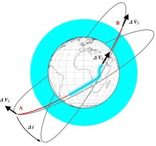
The strategy for the maneuver (Figure 3) involves the combined use of aerodynamic maneuvering in the atmosphere and exoatmospheric propulsion phases. The propulsive phases are assumed to be concentrated in three impulses in space, whereas the portion of atmospheric flight is performed without the use of the propulsion system. The first propulsive impulse (deorbit impulse) at the altitude H_A

of the initial LEO varies the vehicle’s speed by V₁ to enter the atmosphere along an elliptic orbit segment. The second impulse (boost impulse) is applied upon exit from the atmosphere to achieve the final LEO by re-ascending along an elliptic orbit segment. The boost is expressed by the speed variation of the vehicle V₂. The third and final

impulse (circularizing impulse) varies the speed by V3 to

circularize the vehicle’s path within the altitude HB of the

final LEO. The change in the orbital inclination is assumed to be obtained entirely in the atmospheric phase of flight during which the vehicle performs the requested change with optimal control and subject to the imposed heating constraints. In this case, both the constraint on the variation of the inclination of the orbital plane (i) and the constraint on the entering heat flux (HF) are present in the ff expression.









A

B

Equation (1), specified for this case, is expressed as follows:

HF , f HF i

, f i ini , ve

fin , ve

m w R w R

m m w

ff   _{ }  (2)

The convenience of the aeroassisted maneuver must be assessed with respect to the classic “purely propulsive” maneuver, in which the required inclination change is produced by a single propulsive impulse outside of the atmosphere. Incidentally, this maneuver is generally extremely expensive from a propulsive point of view because the V to be applied is proportional to the elevated circular velocity of the spacecraft. The main parameters adopted for the GA are summarized in Table II.

TABLEII GAMAIN PARAMETERS

Number of individuals in the population 100 Number of generations 200 Number of genes 5 Crossover probability 0.85 Initial mutation rate 0.005 Minimum mutation rate 0.0005 Maximum mutation rate 0.25 Relative fitness differential 1.0

The selected state variables for the optimization procedure include the V₁ used to deorbit, the time history of both the bank angle and the angle of attack, and, if required, the transit time in the atmosphere. In this study, the latter was retained as a free parameter with an upper

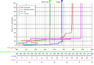
limit, beyond which the mission is considered to be a failure. This hypothesis serves to exclude runs in which the vehicle flies by gliding up and down for a long period of time without sufficient energy to exit the atmosphere. The total initial mass of the vehicle is the sum of the propellant mass, the thermal protection system (TPS) mass, and the structural and payload masses. The goal of the current optimization problem is to perform the orbital plane change while minimizing the sum of the mass of the propellant and the mass of the required TPS. The objective function, which must be maximized, is given by the final mass of the vehicle, which can be defined as the performance index of the problem. Figure 4 shows the trends of the two constraints, the entering heat flux (green) and the variation of the orbital plane inclination (blue), as well as the increase in the final mass (mass gain) to be optimized (red) and the conventional value for the fitness function (fuchsia). These are plotted as functions of the number of generations (indicated as the ordinate). Although the starting “best individual” (the best of population “0” that is passed to population “1” due to elitism) is far from the imposed constraints, the algorithm yields the optimal solution after only a few generations. First, the algorithm attempts to respect the constraints and subsequently maximizes the mass gain, i.e., the saved mass compared with the purely propulsive case. After approximately thirty generations, both constraints are “trapped” by the method (assigned tolerances equivalent to 0.1 deg and 1 W/cm2); the search for the maximum gain in the final mass (red curve with increasing trend) begins from this point.

In practice, the power of this form of the fitness function and reward factor is represented by the adequate distancing on the fitness scale of the solution that complies with the constraints. Subsequently, the improvement is assigned to the selection by the roulette wheel, and the evolution is managed while remaining firmly anchored to the “track” of compliance with the constraints. The adoption of this stepped pyramidal function is not limited to orbital optimization problems and can be effectively employed in other fields of optimization.

VI. CONCLUSIONS

In the context of a global optimization method based on a GA, a method was introduced to consider the constraints of the problem using appropriate stepped pyramidal functions that serve as reward factors in the formulation of the fitness function of the problem. The efficiency of the presented solution was verified in an optimization problem of an orbital aeroassisted maneuver with thermal and dynamic constraints. The findings demonstrate the initial rapid convergence of the solution with regard to compliance with the constraints and subsequently toward the maximization of the objective function of the problem. The entire method and the characteristics of the developed reward factors can be of great benefit for general use in the optimization field of constrained problems.

NOMENCLATURE

A

H = altitude of the initial LEO, m

atm

H = altitude of the sensible atmosphere, m

B

H = altitude of the final LEO, m

fin , ve

m = final vehicle mass, kg

ini , ve

m = initial vehicle mass, kg

in

Q = entering heat flux, W/m2

max , in

Q = maximum entering heat flux, W/m2

A

R = initial LEO radius, m

B

R = final LEO radius, m

j , f

R = reward factor for the component j

HF , f

R = reward factor for the heat flux

i , f

R _ = reward factor for the variation of the orbital

inclination

HF

w = multiplicative weight for the heat flux

j

w = multiplicative weight for the component j

m

w = multiplicative weight for the mass ratio (objective function)

objf

w = multiplicative weight for the objective function

i

w_ = multiplicative weight for the variation of the orbital inclination

lim , BL

T = bond-line limit temperature, K

i

 = variation of the orbital inclination, rad

V

 = total impulse, m/s

1 V

 = deorbit impulse, m/s

2 V

 = boost impulse, m/s

3 V

 = circularizing impulse, m/s

REFERENCES

[1] Herman, A. L., and Conway, B. A., “Direct Solutions Of Optimal Orbit Transfers Using Collocation Based On Jacobi Polynomials”, AAS Paper No.94-126, AAS/AIAA Space Flight Mechanics Meeting, Cocoa Beach, FL, February, 1994.

[2] Seywald, H., “Trajectory Optimization Based on Differential Inclusion”, Journal of Guidance, Control, and Dynamics, vol. 17, no. 3, pp. 480–487, 1994.

[3] Casalino, L., Colasurdo, G., and Pastrone, D., “Optimal Aeroassisted GEO-TO-LEO Transfer By An Indirect Method”, AAS Paper No.95-450, AAS/AIAA Astrodynamics Specialist Conference, Halifax, Nova Scotia, Canada, August, 1995.

[4] Calise, A. J., and Gath, P. F., “Optimization of launch vehicle ascent trajectories with path constraints and coast arcs”, Journal of Guidance, Control and Dynamics, vol. 24, no. 2, 2001, pp. 296–304. [5] Rajesh, K. A., “Reentry Trajectory Optimization: Evolutionary

Approach”, AIAA Paper 2002-5466.

[6] Igarashi, J., and Spencer, D. B., “Optimal Continuous Thrust Orbit Transfer Using Evolutionary Algorithms”, Journal of Guidance, Control and Dynamics, vol. 28, no. 3, 2005, pp. 547–549.

[7] Holland, J. H., Adaptation in Natural and Artificial Systems, University of Michigan Press, Ann Arbor, MI, 1975.

[8] Mazzaracchio, A., and Marchetti, M., “Effect of Spacecraft Aerodynamics and Heat Shield Characteristics on Optimal Aeroassisted Transfer”, Engineering, vol. 4, no. 6, June 2012, pp. 307–320. doi: 10.4236/eng.2012.46040

[9] Mazzaracchio, A., “Thermal Protection System and Trajectory Optimization for Orbital Plane Change Aeroassisted Maneuver”,

Journal of Aerospace Technology and Management, vol. 5, no. 1,

January-March 2013, pp. 49–64. doi: 10.5028/jatm.v5i1.208 [10] Yeniay, Ö, “Penalty Function Methods for Constrained Optimization