University of Pennsylvania University of Pennsylvania
ScholarlyCommons
ScholarlyCommons
Publicly Accessible Penn Dissertations
2019
Methods For Robust Quantification Of Rna Alternative Splicing In
Methods For Robust Quantification Of Rna Alternative Splicing In
Heterogeneous Rna-Seq Datasets
Heterogeneous Rna-Seq Datasets
Scott Simon Norton
University of Pennsylvania, [email protected]
Follow this and additional works at: https://repository.upenn.edu/edissertations
Part of the Bioinformatics Commons
Recommended Citation Recommended Citation
Norton, Scott Simon, "Methods For Robust Quantification Of Rna Alternative Splicing In Heterogeneous Rna-Seq Datasets" (2019). Publicly Accessible Penn Dissertations. 3460.
Methods For Robust Quantification Of Rna Alternative Splicing In Heterogeneous
Methods For Robust Quantification Of Rna Alternative Splicing In Heterogeneous
Rna-Seq Datasets
Rna-Seq Datasets
Abstract Abstract
RNA alternative splicing is primarily responsible for transcriptome diversity and is relevant to human development and disease. However, current approaches to splicing quantication make simplifying assumptions which are violated when RNA sequencing data are heterogeneous. Influences from genetic and environmental background contribute to variability within a group of samples purported to represent the same biological condition. This work describes three methods which account for data heterogeneity when detecting differential RNA splicing between sample groups. First, a robust model is implemented for outlier detection within a group of purported replicates. Next, large RNA-seq datasets with high within-group variability are addressed with a statistical approach which retains power to detect changing splice junctions without sacricing specicity. Finally, applying these tools to call sQTLs in GTEx tissues has identified splicing variations associated with risk loci for cardiovascular disease and anomalous skeletal development. Each of these methods correctly handles the properties of heterogeneous RNA-seq data to improve precision and reduce false discovery rate.
Degree Type Degree Type
Dissertation
Degree Name Degree Name
Doctor of Philosophy (PhD)
Graduate Group Graduate Group
Genomics & Computational Biology
First Advisor First Advisor
Yoseph Barash
Second Advisor Second Advisor
Hongzhe Lee
Keywords Keywords
heterogeneous, methods, outlier, qtl, rna, splicing
Subject Categories Subject Categories
METHODS FOR ROBUST QUANTIFICATION OF RNA ALTERNATIVE SPLICING IN HETEROGENEOUS RNA-SEQ DATASETS
Scott Norton
A DISSERTATION
in
Genomics and Computational Biology
Presented to the Faculties of the University of Pennsylvania
in
Partial Fulfillment of the Requirements for the
Degree of Doctor of Philosophy
2019
Supervisor of Dissertation
Yoseph Barash, Associate Professor of Genetics
Graduate Group Chairperson
Benjamin Voight, Associate Professor of Genetics
Dissertation Committee
Hongzhe Li, Professor of Biostatistics (chair)
Junhyong Kim, Professor of Biology
METHODS FOR ROBUST QUANTIFICATION OF RNA ALTERNATIVE SPLICING
IN HETEROGENEOUS RNA-SEQ DATASETS
c
COPYRIGHT
2019
Scott S. Norton
This work is licensed under the
Creative Commons Attribution
NonCommercial-ShareAlike 3.0
License
To view a copy of this license, visit
ABSTRACT
METHODS FOR ROBUST QUANTIFICATION OF RNA ALTERNATIVE SPLICING
IN HETEROGENEOUS RNA-SEQ DATASETS
Scott Norton
Yoseph Barash
RNA alternative splicing is primarily responsible for transcriptome diversity and is relevant
to human development and disease. However, current approaches to splicing quantification
make simplifying assumptions which are violated when RNA sequencing data are
hetero-geneous. Influences from genetic and environmental background contribute to variability
within a group of samples purported to represent the same biological condition. This work
describes three methods which account for data heterogeneity when detecting differential
RNA splicing between sample groups. First, a robust model is implemented for outlier
detection within a group of purported replicates. Next, large RNA-seq datasets with high
within-group variability are addressed with a statistical approach which retains power to
detect changing splice junctions without sacrificing specificity. Finally, applying these tools
to call sQTLs in GTEx tissues has identified splicing variations associated with risk loci
for cardiovascular disease and anomalous skeletal development. Each of these methods
correctly handles the properties of heterogeneous RNA-seq data to improve precision and
TABLE OF CONTENTS
ABSTRACT . . . iii
LIST OF TABLES . . . vii
LIST OF ILLUSTRATIONS . . . ix
CHAPTER 1 : Introduction . . . 1
1.1 Splicing biology . . . 1
1.1.1 Eukaryotic mRNA transcripts are processed by the spliceosome . . . 1
1.1.2 Alternative splicing contributes to proteomic and functional diversity 3 1.2 RNA splicing quantification . . . 4
1.2.1 Important technological developments for measurement of RNA abun-dance . . . 4
1.2.2 RNA-seq-based methods facilitate high-throughput quantification and de-novo discovery of splicing variations . . . 6
1.2.3 Splicing quantification from RNA-seq relies on the underlying model 7 CHAPTER 2 : Outlier detection and methods evaluations . . . 15
2.1 Introduction . . . 15
2.1.1 What is an outlier in the context of RNA alternative splicing? . . . 16
2.1.2 How is outlier detection typically performed in the literature, and what are the possible shortcomings therein? . . . 17
2.2 Algorithm . . . 17
2.2.1 If we had some weights, how would we use them in MAJIQ? . . . . 17
2.2.2 L1 divergence between P(PSI) and group median . . . 19
2.2.4 Expected (replicates) distribution of L1 divergences, and how it is
used to construct local weights . . . 21
2.2.5 Synthetic introduction of an outlier into an otherwise clean dataset . 22 2.3 Evaluation metrics . . . 22
2.3.1 Reproducibility ratio . . . 23
2.3.2 Intra-to-Inter Ratio . . . 24
2.3.3 Real data . . . 25
2.3.4 Synthetic data . . . 25
2.3.5 Comparison to biochemical assays (RT-PCR) . . . 26
2.4 Results . . . 27
2.4.1 The impact of an outlier on differential splicing predictions and re-producibility . . . 27
2.4.2 Comparison between methods on synthetic data . . . 28
2.4.3 Comparison between methods on real data . . . 31
2.4.4 Evaluating method performance . . . 32
2.5 Discussion and conclusions . . . 36
CHAPTER 3 : Large heterogeneous datasets . . . 42
3.1 Introduction . . . 42
3.2 Algorithm . . . 45
3.2.1 Behavior on toy data . . . 47
3.3 Evaluations . . . 48
3.3.1 Reproducibility in GTEx . . . 48
3.3.2 IIR in GTEx . . . 48
3.3.3 Overlaps between tests . . . 49
3.4 Simulated data . . . 50
3.5 Discussion and conclusions . . . 51
4.1 Introduction . . . 54
4.1.1 Genome-wide association studies and QTL studies . . . 54
4.2 Cardiovascular disease . . . 57
4.2.1 Methods . . . 58
4.2.2 Results . . . 58
4.3 Skeletal growth in children is GWAS-mapped to a locus physically located near an alternative splice site . . . 60
4.3.1 Methods . . . 62
4.3.2 Results . . . 64
4.4 Discussion and conclusions . . . 70
CHAPTER 5 : Conclusions . . . 72
APPENDIX . . . 76
LIST OF TABLES
TABLE 1 : validations 51pct.tsv . . . 77
TABLE 2 : validations 100pct.tsv . . . 77
LIST OF ILLUSTRATIONS
FIGURE 1 : Cartoon illustrating mRNA alternative splicing . . . 4
FIGURE 2 : CYP11B1 as an example of a complex gene locus . . . 9
FIGURE 3 : Figure 1a from Li et al. (2018) . . . 11
FIGURE 4 : Classical binary events . . . 14
FIGURE 5 : Overview of the LSV model . . . 14
FIGURE 6 : Distribution of L1 divergences . . . 23
FIGURE 7 : Synthetic perturbation of tissue replicates . . . 29
FIGURE 8 : Evaluation using “realistic” synthetic datasets . . . 30
FIGURE 9 : Evaluation using real data . . . 33
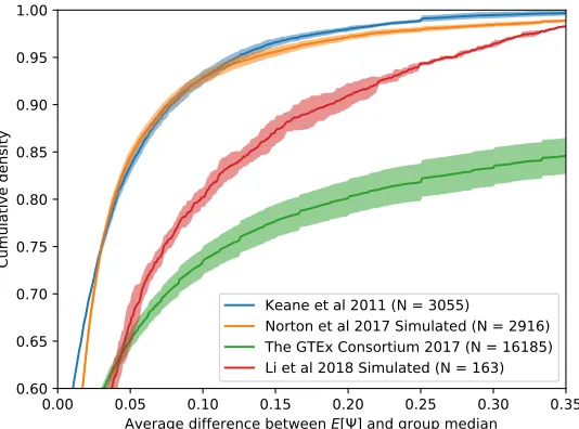
FIGURE 10 : Reproduction of Figure 2 from Li et al. (2018) . . . 36
FIGURE 11 : Comparative evaluation . . . 39
FIGURE 12 : Distribution of absolute deviations in empirical Ψ . . . 41
FIGURE 13 : Toy example for MAJIQ-HET stats . . . 47
FIGURE 14 : Reproducibility of splicing quantifiers on GTEx . . . 48
FIGURE 15 : Reproducibility of splicing quantifiers on GTEx without ∆Ψ filter 49 FIGURE 16 : Intra-to-inter ratio, MAJIQ vs MAJIQ-HET . . . 50
FIGURE 17 : Intra-to-inter ratio on small datasets . . . 51
FIGURE 18 : Intra-to-inter ratio on large datasets . . . 51
FIGURE 19 : Upsets on large datasets . . . 52
FIGURE 20 : Upsets on small datasets . . . 52
FIGURE 21 : Upset of all putative arterial sQTLs . . . 60
FIGURE 22 : Upset of GWAS-implicated putative arterial sQTLs . . . 61
FIGURE 23 : Diagram ofADAMTS7 . . . 61
FIGURE 25 : Example case of abnormal skeletal growth . . . 66
FIGURE 26 : Association between rs6410 andCYP11B1 exon 4 inclusion . . . 67
FIGURE 27 : Raw RNA-seq reads atCYP11B1 exon 4 . . . 67
FIGURE 28 : Association between rs6392 andCYP11B1 alternative 3’SS . . . . 68
FIGURE 29 : Raw RNA-seq reads itCYP11B1 exon 9 . . . 68
FIGURE 30 : RT-PCR ofCYP11B1 intron 3 retention . . . 69
CHAPTER 1 : Introduction
This section reviews the fundamentals of RNA splicing biology, the tools and technologies
that exist to measure RNA splicing in tissues and changes between tissues, and the inherent
challenges that are addressed by the work supporting the later chapters.
1.1. Splicing biology
1.1.1. Eukaryotic mRNA transcripts are processed by the spliceosome
Gene expression is the essential mechanism by which a cell synthesizes the proteins it needs
to function. These proteins are encoded as genes in the cell’s DNA, which are transcribed
into messenger RNA (mRNA) by an RNA polymerase (RNA Polymerase II in mammals)
and translated into proteins by ribosomes. Cells have additional layers of regulation on top
of this, which allow it to control the abundance of each protein to adapt to its immediate
needs. In complex organisms, the patterns of regulation vary between cell types and result
in different genes being expressed at different levels, which results in differences in cellular
function.
Eukaryotes in particular have a complex gene structure, with its sequence consisting of
“exons” and “introns”. In general, mature mRNAs consist of only exons, which contain the
linear sequence that directly encodes for the protein product. As such, the introns must
be removed from the nascent mRNA transcript (pre-mRNA), and the process by which
this occurs is called “splicing”. During processing of the pre-mRNA, which commonly
occurs co-transcriptionally (Herzel et al., 2017), a complex of RNA and proteins called the
“spliceosome” assembles on the nascent RNA transcript at specific points on the intron
and flanking exons. The components of this machinery and the process it mediates are
summarized in a review by Matlin et al. (2005). Briefly, the spliceosome contains five
catalytic small nuclear ribonucleoproteins (snRNPs) termed U1, U2, U4, U5, and U6 in
complex with large proteins. The assembly of the basal spliceosome is guided by consensus
motifs at the 5’ (recognized by U1) and 3’ (recognized by U2 auxiliary factor (U2AF))
upstream from the 3’ splice site, bound by splicing factor 1 (SF1)) and an 18+-residue
polypyrimidine tract at the 3’ end of the intron (also bound by U2AF). Additional splicing
regulatory proteins (SRps), such as those in the CELF and RBFOX families (Sun et al.,
2012; Chen and Manley, 2009; Gazzara et al., 2017), can bind to the mRNA, either in the
intron or in either flanking exon, to enhance or inhibit spliceosomal assembly and activity.
Once formed, the basal spliceosome recruits additional RNAs and proteins, including U2
snRNP itself, to bring the 5’ and 3’ splice sites into proximity with one another. This
proximity mediates the ATP-driven excision of the intron in two major catalytic steps:
nucleophilic attack of the branch point adenine on the 5’ splice site, cleaving the 5’ end and
creating the lariat intermediate; and nucleophilic attack of the 3’ end of the upstream exon
on the 3’ splice site (which also has a conserved sequence motif), freeing the intron from
the rest of the transcript and joining the exons together (Herzel et al., 2017). This process
is repeated iteratively for each intron to be removed.
Splicing is one of three major forms of post-transcriptional or co-transcriptional processing
of mRNAs in eukaryotes (Beyer and Osheim, 1988; Tilgner et al., 2012; Ameur et al., 2011).
It is also essential for the 5’ end of the transcript to be “capped” with a 5-methylguanine
residue. This 5’ cap is recognized by the eukaryotic translation initiation complex
(specifi-cally, by a protein called EIF4F in humans), and is therefore required for the protein to be
translated. Additionally, the 3’ end of the transcript is adorned with a polyadenosine
(poly-A) tail. This tail is associated with transcript stability in both eukaryotes and prokaryotes.
In eukaryotes, it serves as the binding substrate for poly-A binding proteins (PABP).
mRNAs are not the only class of transcripts subject to this processing. Recently, several
long noncoding RNAs (lncRNAs) have been classified. These RNA Polymerase II products
are capped, spliced, and polyadenylated in the same manner as mRNAs. However, as
the name suggests, the mature transcripts do not code for any protein product, nor are
they exported to the cytoplasm where the ribosomes reside. Instead, the mature lncRNA
chromatin and transcriptional regulation (Cao, 2014).
1.1.2. Alternative splicing contributes to proteomic and functional diversity
Differential binding of the aforementioned SRps affect the degree to which a given splice
site is used. The consequence of this is the differential inclusion and exclusion of exons
and exonic segments in the mature transcript, a phenomenon termed “alternative splicing”.
Figure 1 depicts a toy example of a gene with two transcript isoforms, one in which the
red exon (circled) is included, and one where it is skipped. The functional consequence is
the presence or absence of the red domain on the protein product. If, for example, this
red domain is a ligand binding site, the choice of whether to include or skip the coding
exon will affect the response of the protein product to that ligand, which impacts how the
cell as a whole responds to stimulus. In some cases, an alternative transcript may not
yield a viable protein product at all. This usually happens because the alternative
tran-script has a premature termination codon, introduced either in the alternatively included
exon or intron, or as a result of a frame shift. These transcripts are normally targeted for
nonsense-mediated decay (NMD) (Lykke-Andersen and Jensen, 2015). Additionally,
alter-native splicing can result in differential inclusion of regulatory domains on the mRNA itself,
such as RNA-binding protein (RBP) and micro RNA (miRNA) binding sites, whether due
to sequence alone or a change in the mRNA’s secondary structure that affects binding of
the aforementioned. While this change would not affect the translated protein product, it
does impact where the protein is expressed and at what level.
Alternative splicing is particularly abundant in higher mammals, with an estimated 90% of
multi-exon genes in humans, both coding and non-coding (Deveson et al., 2017), showing
evidence of multiple transcript isoforms (Wang and Cooper, 2007). Many of these
alterna-tive isoforms are cell-type specific, and the regulation of alternaalterna-tive isoform expression is
tightly regulated during various stages of organism development. Moreover, dysregulation
of alternative splicing has been observed in several diseases, including familial and sporadic
forms of frontotemporal dementia (FTD) and Alzheimer’s disease, and various cancers
Figure 1: Cartoon illustrating mRNA alternative splicing. The red exon (circled) can either be spliced in to yield the top isoform or spliced out to yield the bottom isoform. Each isoform is translated into a different protein, one with the red domain, and one without.
Colak et al., 2013; Dvinge and Bradley, 2015). In order to better understand the precise
mechanisms driving alternative splicing differentiation and disease, it is necessary to
accu-rately quantify splicing in tissue samples and measure splicing changes between biological
or experimental conditions.
1.2. RNA splicing quantification
RNA splicing quantification is a rapidly evolving field accelerated by the advent of RNA-seq
in 2008 (Nagalakshmi et al., 2008; Mortazavi et al., 2008). This chapter summarizes some
of the major technological developments in measuring RNA levels in tissue extracts, and
the evolution of methods for quantifying alternative splicing.
1.2.1. Important technological developments for measurement of RNA abundance
Prior to the advent of RNA-seq, two biochemical techniques predominated for
measur-ing RNA alternative splicmeasur-ing. The higher-throughput of these is the microarray, in which
fluorescently-labeled DNA oligonucleotides (oligos) anneal to complementary RNAs.
Alter-native transcript abundance for a given gene can be measured by designing two or more
probes with different fluorescent tags, each complementary to a sequence unique to one of
the transcript isoforms. After washing away unbound probes, the abundance of each isoform
can be interpreted by imaging from the relative intensity of each fluorescent frequency. This
technique can be performed for multiple genes or multiple samples in parallel by loading
detect by reverse-transcribing (RT) the mRNA transcript to complementary DNA (cDNA)
followed by a polymerase chain reaction (PCR) to amplify the cDNA product (RT-PCR).
The microarray technique has some technical limitations. First, the throughput of the
technique is restricted to the number of wells on the wellplate used for the analysis.
Addi-tionally, because the hybridization probes must be designed before the microarray analysis
is performed, this technique cannot be used forde novodiscovery of splice isoforms. Lastly,
the fluorescent intensity can be difficult to interpret in a quantitative fashion - the signal
can either be too low for the sensor to distinguish from background, potentially resulting
in false negative detection, or so high that it saturates the sensor, frustrating differential
analysis.
Carefully-performed RT-PCR is a popular low-throughput technique for local splicing
quan-tification and is considered to be the gold standard among biochemical assays. RT-PCR
primers are designed to flank an alternative splicing event, which is defined in terms of
the alternatively-included exon, exonic fragment, or retained intron. Classically, splicing
events include cassette exons, alternative 5’ donor or 3’ acceptor sites, mutually exclusive
exons, and intron retentions, as depicted in Figure 2. RT-PCR is assessed by measuring
the relative intensity of two or more bands on a Northern blot, which correspond to the
known fragment sizes for each splice form. In the case of a cassette event, amplified
frag-ments including the alternative exon will be larger and migrate less distance on the gel than
fragments skipping the exon. The relative intensities of the two bands are summarized as a
single quantity PSI (Ψ), or “percent spliced in”, for the alternative fragment. Splicing can
be directly compared between two experimental conditions as the change in Ψ (Delta PSI,
∆Ψ). This approach is advantageous in that it accurately captures local splicing decisions
in a quantitative fashion. However, RT-PCR is labor-intensive and low-throughput, and
1.2.2. RNA-seq-based methods facilitate high-throughput quantification and de-novo
discov-ery of splicing variations
The advent of high throughput sequencing (Next-Generation Sequencing, or NGS) has
rev-olutionized quantitative genomic and transcriptomic analysis. The predominant variation
of this is the sequencing-by-synthesis technique employed on the Illumina platform. This
technology directly reads the nucleotide sequences of each DNA molecule in the input
sam-ple. These “reads” can be mapped back to a reference genome or transcriptome using tools
such as BowTie (Langmead et al., 2009), STAR (Dobin et al., 2013), or HISAT2 (Kim et al.,
2015).
The technique itself, which is described in detail by Solexa Ltd. (Bennett, 2004; Slatko et al.,
2018), requires special preparation of a DNA or cDNA library to produce DNA molecules
to average 300 nucleotides in size with specialized adapters annealed to the 3’ end of each
molecule. The library is loaded onto a flow cell, which contains billions of clusters of
oligonucleotides complementary to these adapters. The DNA is amplified on these clusters
by the sequencer using the oligos as PCR primers. The final round of amplifcation is
modified to add one fluorescently-labeled nucleotide at a time, up to a predetermined,
protocol-dependent length. When incorporated, the sequencer reads the fluorescent signal
simultaneously for all clusters on the flow cell, and interprets the sequence of images as the
original DNA sequence at each cluster.
One key advantage of this technology is that each molecule in the input sample can be
mapped directly to at most one read in the output. When multiple molecules originate
from the same genomic region, the relative representation of that region can be interpreted
from the number of reads mapping back to it. This is a digital count which, unlike
fluo-rescent signal detection, has no upper bound, thus enabling the accurate quantification of
both lowly-expressed and highly-expressed loci. Additionally, splice-aware mappers such as
STAR and HISAT2 can map RNA reads to the genome instead of a transcriptome, allowing
transcript model.
A second benefit of high-throughput sequencing is that it can be multiplexed, allowing for
the simultaneous evaluation of multiple samples. Multiplexing is achieved by incorporating
unique DNA “barcodes” into the adapters annealed to the amplified DNA in each sample.
During the image processing step, the sequencer separates the reads using the barcode as a
key for which sample the reads originally came from.
High-throughput sequencing, including RNA-seq, is not without its limitations. First,
be-cause library preparation is a multistep process with the potential for loss at each step,
some molecules from the original extract may not appear in the sequencer output. This is
evidenced by an apparent read, fragment, or transcript count of 0 for some genomic regions
(zero-inflation) (Rashid et al., 2011). Since the same can arise due to the molecule being
absent in the original tissue sample (i.e. the gene or transcript is not expressed), zero counts
must be interpreted with caution. Each step of the process additionally incorporates its
own systematic biases, including a positional bias favoring the 3’ end of transcripts and a
bias towards sequences with high GC content. Finally, NGS technologies are designed to
produce only short sequencing reads, typically between 100-150 bp in length. While this is
sufficient to estimate gene expression, it makes quantification of whole transcript isoforms
challenging. Sequencing the cDNA from both ends (paired-end sequencing) improves
map-ping accuracy, but the gains in performance for transcriptome quantification and assembly
are modest (Song and Florea, 2013). These technical shortcomings must be addressed when
processing RNA-seq experiments for expression or splicing quantification.
1.2.3. Splicing quantification from RNA-seq relies on the underlying model
Isoform quantifiers
Several tools and models have been proposed to address the unique challenges posed by
using RNA-seq for transcript and splicing quantification. Chief among these are methods
such as SALMON (Patro et al., 2017) and RSEM (Li and Dewey, 2011) which attempt to
a transcript model and attempt to assign RNA-seq reads to transcripts. This is more
easily done in simple cases where two alternative transcripts share all but a small number
of exons or parts of exons. However, many genes have three or more transcripts, some of
which mutually share exons and splice junctions. TheCYP11B1 locus, for example, has five
annotated transcript isoforms with substantial local overlap in sequence. In particular, the
three longest isoforms are nearly impossible to distinguish from the two shortest isoforms
given only reads starting within exon 9 (see Figure 2). Therefore, these algorithms must
determine what fraction of reads mapping to shared exons come from which transcript
isoforms.
Both RSEM and SALMON construct a joint parametric model of transcript abundance and
read assignments to transcripts, and use expectation maximization (EM) to optimize this
model. In EM, observations (reads) are first assigned their expected class labels (transcripts)
based on the current state of the model parameters. Next, the parameters are updated
to values which maximize the total likelihood of the joint model given the current label
assignments. In the simplest case, the total number of reads assigned to a transcript is
scaled (normalized) by the number of mappable positions on that transcript. The maximum
likelihood estimate is then the fraction of normalized reads for each transcript
(transcript-level expression) relative to the sum of normalized reads for all transcripts at that locus
(total gene expression). The two steps of label assignment (expectation) and parameter
update (maximization) are repeated until the joint likelihood of the model converges. The
final optimized parameters are then used to provide transcript-level expression estimates as
transcripts per million RNA molecules (TPM).
In general, transcript levels are highly informative of biological activity in cells. However,
the task of quantifying isoform expression transcriptome-wide is complicated by the problem
of de-novo transcript assembly from short RNA-seq reads. The main barrier to accurate
transcriptome assembly from NGS data is determining whether two distant exons originate
technologies such as PacBio and Oxford Nanopore. However, the current cost of running
these platforms is still considerably high for decent coverage. Moreover, these technologies
are more useful for detecting isoforms in the task of transcriptome definition than for isoform
quantification.
Figure 2: CYP11B1 as an example of a complex gene locus. Image lifted from the UCSC hg19 Genome Browser, ”UCSC Genes” track, zoomed to cover the CYP11B1 locus on chromosome 8q24.3. The region in the red box highlights parts of exons 9-11. Reads originating from fragments mapping here can be used to distinguish between the three long and two short isoforms, but cannot be assigned to any one transcript. In particular, it is not possible to distinguish between isoforms 3 and 5 from these reads alone, as they do not capture the inclusion of exon 4.
Event quantifiers
Several methods for RNA quantification avoid the problem of transcript assembly altogether
by framing RNA splicing in a more local context. The premise is that alternative splicing
results in the alternative inclusion or exclusion of exons. In many cases, this affects the
differential presence of functional or structural domains in the translated protein product
or on the mRNA itself. The fraction of the RNA sample that includes the alternative exon,
relative to the number of reads which exclude the exon, is often reported as the “percent
spliced in” (Ψ) for that exon.
The alternative exclusion of whole exons is called “exon skipping” or a “cassette exon
event”, and is one of several classically-defined “splicing event” types in the literature (Wang
et al., 2015). Other event types include alternative 5’ splice sites, alternative 3’ splice sites,
mutually exclusive exons, and intron retention. These are depicted in Figure 4. These events
are much easier to define from NGS data because they rely only on reads mapping uniquely
to each variant of the event. Methods such as rMATS (Shen et al., 2014) and MISO (Katz
et al., 2010) were developed to quantify Ψ for splicing events transcriptome-wide.
Some methods, such as SUPPA (Entizne et al., 2016; Trincado et al., 2018), take a hybrid
quantifica-tions. This approach takes normalized transcript counts (number of copies of each transcript
per million of reads sequenced, or TPM) as estimated by SALMON or RSEM and, for each
event, combines counts from all transcripts containing the same variation of the event to
estimate Ψ. For example, in an exon skipping event, Ψ is estimated as the ratio between the
sum of all TPM from transcripts containing the cassette exon and the sum of TPM from all
transcripts annotated at that gene locus. While this resolves the ambiguity problem faced
by SALMON and RSEM alone, it does not facilitate de-novo junction discovery.
While event quantifiers are fast and accurate, the definition of these events is limited in its
ability to describe the full complexity of mammalian transcriptomes. Indeed, as much as
30% of observed transcriptome variations cannot be correctly quantified under this
frame-work because they do not fit the underlying events model (Vaquero-Garcia et al., 2016).
Notably, both rMATS and MISO rely on a user-provided transcriptome annotation from
which splicing events are constructed. As a consequence, they do not detect novel splicing
events (de-novo detection), which limits their ability to discover new splicing biology. The
ability to detect de-novo splicing variations is important for studying low-abundance or
developmentally-transient cell types as well as diseases affecting splicing regulation.
Cluster quantifiers
A third, more recent class of methods approaches the problem as one of junction or intron
clustering. This approach groups alternative transcripts by the set of junctions or introns
that share splice sites between them (see Figure 3). Methods following this approach include
Whippet (Sterne-Weiler et al., 2018) and LeafCutter (Li et al., 2018). This represents a
generalization on the classical event model in that splice junctions sharing at least one
flanking constitutive exon between them can be explained as a single splicing event covering
differential usage of subsets of junctions. This model reflects the observation that RNA
splicing occurs via the “stepwise removal of introns from nascent pre-mRNA”. Because
this model examines splicing locally and is not constrained by classical event definitions,
it can accurately quanitfy the remaining 30% of transcriptome complexity that is omitted
Figure 3: Figure 1a from Li et al. (2018). Differentially-excised introns are identified from spliced reads as flagged by the RNA-seq mapper. A cluster is defined from all excised introns which share at least one splice site.
unannotated exons and splice junctions from the input reads. Importantly, LeafCutter was
designed for the discovery of splicing quantitative trait loci (sQTLs), allelic variants which
associate with changes in splicing. However, neither approach detects unannotated or de
novo retained introns, the likes of which are present in both normal (Schmitz et al., 2017)
and disease (Dvinge and Bradley, 2015) tissue contexts.
Local splicing variation quantifier
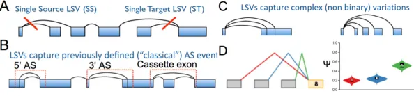
The fourth class of methods explains alternative splicing in terms of “LSVs”, which are
conceptually similar to the aforementioned cluster-based models. The LSV definition can
be interpreted by visualizing a gene model as a directed (5’ to 3’) graph, where the edges
splice junctions. An LSV is defined as a split in this graph representing an individual
splicing decision at a single splice site (Figure 5A). This framework naturally captures all the
variations explained by classical binary splicing events (Figure 5B) but have the flexibility
to describe non-classical and complex (3 or more splice junctions, Figure 5C) events that are
misclassified or excluded by classical models. Additionally, alternative junction inclusion
levels can be quantified from RNA-seq in a manner similar to traditional Ψ quantification.
MAJIQ (Model of Alternative Junction Inclusion Quantification) was developed around the
LSV framework (Vaquero-Garcia et al., 2016; Norton et al., 2018). MAJIQ works by first
building a splice graph model for each gene in the supplied reference annotation. This model
captures all exons and splice junctions in the transcriptome annotation, and identifies points
where two transcripts converge or diverge as LSVs. Optionally, MAJIQ supplements this
model with evidence from the supplied RNA-seq alignments, adding new splice junctions
and LSVs where there are enough reads to support them. Spliced reads flagged by the
aligner are assigned uniquely to junctions in the splice graph. This process implements
quality control measures such as probabilistic stack removal to remove PCR duplicates and
parametric bootstrapping to capture the per-experiment, per-junction variance in mapped
read levels. Next, a Bayesian model is applied to compute a posterior distribution of Ψ for
each LSV junction using the bootstrapped read counts on top of a Jeffrey’s prior. Evidence
from replicate experiments is accumulated in this step to provide a more confident estimate
of Ψ. An additional Bayesian prior is applied when estimating differential splicing between
conditions. Finally, MAJIQ comes packaged with a visualization suite called VOILA which
generates publication-ready illustrations of the splice graph model, read count distributions,
and Ψ and ∆Ψ quantifications at each LSV (Figure 5D). Additionally, VOILA generates a
human- and machine-readadble TSV file summarizing splicing quantifications at all LSVs.
Of the aforementioned methods that quantify alternative splicing in groups of RNA-seq
experiments, all of them assume that these groups arebona fide replicates of an underlying
groups can be heterogeneous for a number of known and unknown reasons. For instance,
an experiment involving inbred mice can be confounded by differential food consumption
between individual mice, mislabeling of tissue samples, or a shift in environmental
condi-tions between batches of samples. Human population studies pose additional challenges for
splicing quantification, as it is unethical to control for genetic and environmental variation
in the study group the way one would with mice. One can attempt to compensate for this
by expanding the sample size, but the underlying heterogeneity must still be accounted for
properly. Genetic and environmental variants can covary with splicing, making it difficult
to conclude whether an observed splicing variation is the result of the study condition or if
it is confounded with an underlying trait.
The major contributions of this body of work are as follows. First, I developed a method
for detecting splicing outliers in a group of purported replicate experiments. I extended
that method to correct for outlier replicates at the Ψ level. This functionality, described
as MAJIQout, was integrated into MAJIQ and is available starting in version 1.1. As part
of developing MAJIQout we also developed an extensive set of evaluation criteria to assess
algorithms for differential splicing quantification from RNASeq, something the community
lacked. We then applied these tests to state of the art algorithms to assess their performance.
Next, I addressed the impact of data heterogeneity and dataset size on splicing observations,
and developed a framework for detecting differences in alternative splicing between large
heterogeneous sample groups using robust rank-based statistics. We termed this framework
MAJIQ-HET, and it is included as part of MAJIQ 2.0. Finally, I designed a pipeline that
uses MAJIQ Ψ quantifications to call splicing quantitative trait loci (sQTLs). I applied this
pipeline in collaboration with researchers at the University of Pennsylvania, the Children’s
Hospital of Philadelphia, and Erasmus University Medical Center to discover and validate
Figure 4: Schematic depicting some of the classical binary events that are quantified by event-based methods such as rMATS and MISO. From left to right: alternative 5’ (donor) splice site, alternative 3’ (acceptor) splice site, and exon skipping (cassette exon). Not depicted but still relevant are the cases of mutually exclusive exons where the decision is between two options for a cassette exon, and intron retention where the intervening intron is not spliced out.
CHAPTER 2 : Outlier detection and methods evaluations
This chapter details a new approach for outlier detection in RNA alternative splicing
quan-tification, as well as best practices for evaluating and comparing method performance and
accuracy. The original work is published in Norton et al. (2018).
2.1. Introduction
Data from present-day RNA-seq experiments face challenges relating to sequencing depth,
transcriptome coverage, and biological and technical variability (Alamancos et al., 2014).
A popular workaround for this is to sequence multiple replicates of the same experiment.
Replicates can be either “biological” i.e. the data come from different organisms or tissue
samples from the same condition group, or “technical” i.e. the same library is sequenced
more than once. Generally, technical replicates grant consistency in observations and can
improve power to detect true splicing changes. However, a single RNA-seq library can fail to
capture low-abundance transcripts simply by chance. Biological replicate designs overcome
this by constructing multiple libraryies, giving these transcripts a greater likelihood of
representation in at least one experiment.
In each case, the information from replicate data is combined to detect biological signals.
Many RNA splicing and transcript abundance quantifiers are designed to handle multiple
replicates. rMATS (Shen et al., 2014), for example, implements a hierarchical logit-normal
distribution to explain per-replicate Ψ in terms of a group mean Ψ and variance.
MA-JIQ (Vaquero-Garcia et al., 2016), meanwhile, models Ψ using a Bayesian framework where
the read counts bootstrapped from each additional replicate updates a beta posterior model
for the underlying group Ψ. Each of these approaches has its advantages and disadvantages
for Ψ quantification, but both assume that the input samples are true replicates sharing
an underlying distribution of event or junction Ψ. When the data violate that assumption,
neither model is guaranteed to accurately represent the true underlying Ψ.
under-ling Ψ? This dissertation discusses two such scenarios. The first, covered by this chapter,
explores the case where one or more experiments is an outlier replicate. The second,
ex-plained in the next chapter, deals with larger sample groups that are true representatives
of the underlying biological condition but exhibit a great deal of heterogeneity.
2.1.1. What is an outlier in the context of RNA alternative splicing?
Genomic datasets are grainy snapshots of biological samples, so some variance is to be
expected. In addition to the irreducible portion of variance inherent in the technique, there
are also genuine biological reasons why per-sample measurements differ. For bulk tissue
RNA-seq, these can include differences in the cell-type composition of the tissue sample,
fluctuations in gene expression within the sample, and specimen-specific environmental
factors. In light of these known sources of variation, some disagreement between
per-sample quantifications is tolerable. However, per-samples which deviate strongly from the
group consensus - “outliers” - are not.
Statistical outliers with respect to an event are samples in an experiment which significantly
skew the group estimate. Specifically, in the problem of splicing quantification from
RNA-seq experiments, the distribution of mapped reads in an outlier deviates substantially from
those of the remaining experiments in the group. This can manifest in the outlier reporting
different splice junction inclusion levels than its fellow experiments, either relative to other
junctions describing the same splicing event or in terms of total number of reads mapping
to that event (depth of coverage). The impact of a read count outlier is of particular
importance - if an experiment reports much fewer reads than the others in the group, it
can reduce the apparent significance of changes in splicing (∆Ψ) between groups even if the
outlier’s point estimate of Ψ is in agreement with the group.
It is not atypical to observe some background divergence within a group of replicate
ex-periments, even events at which one replicate disagrees quite strongly with the remainder.
What makes a replicate abona fide outlier is the prevalence of such disagreements across the
en-tire transcriptome, accumulating evidence of disagreement with the remaining experiments
in the study group. Therefore, a robust outlier detection algorithm would define a metric of
divergence between each replicate’s quantification of an event and a group representative,
and evaluate this metric on all events to determine whether one replicate is a serial offender
in this regard.
2.1.2. How is outlier detection typically performed in the literature, and what are the possible
shortcomings therein?
Statistical outliers are of significant concern when dealing with biological data, which is
often noisy in and of itself. However, there is little to no discussion in the literature on how
to handle it. Instead, researchers are left to use their own heuristics to determine whether
a sample might be an outlier. Often, these heuristics carry hidden biases which impact
anaylsis. A recent work by Conesa et al. (2016) suggests using PCA to query whether
samples of the same condition cluster together, but admits that “no clear standard exists
for biological replicates” as pertains to measuring within-group consistency. The work
described in this chapter addresses this gap in the literature, and was originally published
as Norton et al. (2018).
2.2. Algorithm
2.2.1. If we had some weights, how would we use them in MAJIQ?
Before we describe our approach to outlier detection, we first explain how such an approach
should be applied in practice. Let us examine the original quantification model on a
collec-tionT ofN experiments representing a biological condition. A splice graph is generated for T by the MAJIQ builder, and the junction-spanning RNA-seq reads from each experiment t∈ T are assigned to LSV junctions. To control for sampling variance in read alignments across positions in the transcript, we bootstrap read counts for each junctions based on the
number of reads starting at each nonzero position that is assigned to the LSV. Let us call
these read counts {Ri,j,t}, where i is the index of the LSV, j is the junction index within
LSVi, and t is the current experiment. Suppose that LSV ihas J splice junctions. Prior
distribution for each j. (The joint distribution of junction Ψ is a Dirichlet(1 J, . . . ,
1 J | {z }
ntimes
).
However, we consider the marginal distribution for each junction separately to make the
model tractable.) Each experimenttcontributesRi,j,t reads of evidence supporting junction
j, and a combined P
j06=jRi,j0,t reads supporting the other junctions. Thus the posterior
distribution of Ψi,j |tis
Ψi,j |t∼Beta
Ri,j,t+
1 J,
X
j06=j
Ri,j0,t+J −1 J
. (2.1)
This posterior can be updated with the read counts from the remaining replicates inT, so that the posterior distribution becomes
Ψi,j | T ∼Beta
X
t∈T
Ri,j,t+
1 J,
X
t∈T
X
j06=j
Ri,j0,t+J −1 J
. (2.2)
Now, suppose we had used some heuristic to estimate for eacht∈ T the probabilityρtthat
t is a bona fide member of T. We can apply this knowledge by scaling the mapped read counts for each junction of each LSV for each trelative to itsρtas such:
Ψi,j | T,{ρt}t∈T ∼Beta
X
t∈T
ρtRi,j,t+
1 J,
X
t∈T
X
j06=j
ρtRi,j0,t+J −1 J
. (2.3)
Theseρt constitute the first computational objective of the outlier detection algorithm.
In practice, each of these three density functions accounts for one set of bootstrapped read
count samples. To account for within-sample variance, this density is computed separately
according to Equation 2.2 for each sample, and all these densities are averaged per LSV
junction. The resulting density is encoded and processed downstream as a vector of binned
2.2.2. L1 divergence between P(PSI) and group median
Here we define our metric for determining how well an experiment agrees with the rest of
the group on junction Ψ. First, we need to determine a suitable representative distribution
for the group consensus Ψ, henceforth labeled (Ψi,j| T). We choose to represent the group
consensus using the group median, as this measure of center is known to be robust to
outliers. To accomplish this, we define how to construct a median density from a set of
random variables.
Definition 1 Suppose a set ofmrandom variables{X1, . . . , Xm}have densitiesP(X1 ≤x) =F1(x)
and so forth. The median of these random variables, denoted X, has density P(X ≤x) = F(x) such that
F−1(q) = med
1≤i≤mF
−1
i (q)
for each 0≤q≤1.
In the event that the random variables in Definition 1 are discrete rather than continuous,
the inverse density functionsFi−1 can be interpolated i.e. linearly without egrigious loss of
precision. The median densityP(Ψi,j ≤ψ| T) can thus be computed from the per-replicate
binned densitiesP(Ψi,j ≤ψ|t).
Next, we define our measure of distance between probability densities. We acknowledge the
existence and widespread use of Kullback-Leibler divergence (KL divergence) to quantify
this. In short, the KL divergence between two discrete probability densities P and Q is
defined as
DKL(P||Q) =−
X
i
P(i) log2
Q(i) P(i)
.
However, we choose not to use KL as our distance metric because it is not bounded above.
Indeed, in a worst case scenario where the two distributions are spike-and-slab densities
with non-overlapping spikes, the KL divergence tends toward positive infinity as the height
of the slab and width of the spike both approach 0. Instead, we employ the L1-divergence
Definition 2 If P and Q are two probabilitiy densities, then the L1 divergence between them is
DL1(P, Q) =
1 2
X
i
|P(i)−Q(i)|.
The divergence measure constructed by this definition has two key properties. First, it is
symmetric with respect to the random variables; that is, DL1(P, Q) = DL1(Q, P), unlike
KL divergence. Second,DL1(P, Q)∈[0,1] for any two probability densitiesP andQ. This
property makes L1 divergence slightly easier to interpret.
Let di,j,t = DL1(Ψi,j | t,Ψi,j | T) be the L1 divergence between the distribution of Ψi,j
informed by experiment t compared to the median density for group T. Because roughly 70% of LSVs are binary in nature, we reduce this to a single value for each LSV by taking
the junction with the maximum L1 divergence, that is,di,t:= max1≤j≤Jdi,j,t.
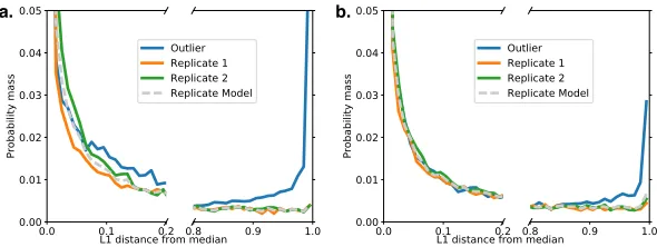
2.2.3. Distribution of L1 divergences, and how it is used to construct global weights
Having computed the di,t for each t ∈ T for each LSV, we can observe how they are
distributed. Figure 6 depicts these distributions for two situations where a group of three
mouse tissue experiments has a known outlier. When the group has no outlier, all three
replicates have the same distribution as Replicate 1 and Replicate 2 (data not shown).
While the distribution of L1 divergences for all three experiments has a spike at 0, only the
outlier has an additional spike at 1, indicating an enrichment in highly-disagreeing LSVs.
We leverage this information in a robust manner by modeling the number of
highly-disagreeing LSVs per LSV. Let Kt be the number of LSVs for which di,t ≥ τ for some
fixed τ, and KT be the size of the union of such LSVs across all experiments in T. In a
study with no outliers, we expect these Kt to be around the same, that is, each replicate
contributes equally to the total disagreement on LSV Ψ in the study. If all the replicates
are “well-behaved”, we could model this with a Binomial distribution, where
where p= 1
N represents the equal proportion of highly-disagreeing LSVs counted for each
replicate. In practice, we observe greater dispersion in Kt than can be explained by a
binomial model. To capture this dispersion, we instead proposed a Beta Binomial model
with p ∼ Beta(Nα, α(1− N1)), where α is a fixed dispersion hyperparameter. Using this model, we can finally express the relative probability ρt that experiment t is a replicate of
the condition underlyingT:
ρt=min 1,
PBB(X > Kt)
PBB(X > KNT)
! ,
where PBB represents the probability of the expression under the aforementioned
beta-binomial model.
2.2.4. Expected (replicates) distribution of L1 divergences, and how it is used to construct
local weights
ρt generated as described can be applied according to Equation 2.3 to globally weight each
experiment’s contribution to junction Ψ proportional to how much we believe each is a true
representative of T. This approach is termed “MAJIQ-gw”. However, Figure 6 indicates that even a strong outlier only disagrees on Ψ for a relatively small number of LSVs. While
this global weighting scheme corrects those events, it comes at the cost of the contribution
the outlier’s reads make towards quantification of the events where it does agree with the
group consensus. To counteract this, we devised a scheme for estimating local (per-LSV)
weights. We start by summarizing the per-experiment distributions ofdi,t into an empirical
model that represents an average replicate of T using theρtas weights:
P(di,T =x) =
P
tρtP(di,t=x)
P
tρt
.
We then define a new variable νi,t to represent the “local” weight for LSVias a likelihood
ratio between the density ofd∗,t andd∗,T in a neighborhood ofdi,t. That is, if we letε >0,
then
νi,t = min
1,P(|X−di,T|< ε) P(|X−di,t|< ε)
Theseνi,t are used in the MAJIQ Ψ quantification model in the same way as the ρt:
Ψi,j | T,{νi,t}t∈T ∼Beta
X
t∈T
νi,tRi,j,t+
1 J,
X
t∈T
X
j06=j
νi,tRi,j0,t+ J−1
J
. (2.4)
This approach of using local weights in MAJIQ is termed “MAJIQ-lw”.
2.2.5. Synthetic introduction of an outlier into an otherwise clean dataset
To benchmark the performance of MAJIQ-gw and MAJIQ-lw for correcting outlier
repli-cates, we devised two strategies for synthetically introducing an outlier into a group of
biological replicate RNA-seq experiments. The first is a replicate swap, in which one
exper-iment in the group is selected at random to be removed and replaced with an experexper-iment
representing a completely different condition or tissue in the same dataset. The second is a
more complex procedure wherein a replicate is transformed to become an outlier. Briefly,
one replicate is selected at random to receive a “synthetic perturbation”. For each LSV with
sufficient read support for quantification, Ψ is quantified for each junction. Next, a random
subset of LSVs, representing a fraction θ of the set of quantifiable LSVs, is selected. For
each LSV in this subset, the expected Ψ (E[Ψ]) for one junction is then shifted by adding or
subtracting a fixedδ. Whether thisδ is added or subtracted is determined by a Bern(E[Ψ])
random variable. The remaining junctions E[Ψ] are scaled linearly such that the E[Ψ] for
all junctions sum to 1. Finally, the original read counts for that LSV are shifted such that
they now explain the new E[Ψ]. To simulate the effect of a read-depth outlier, all read
counts for the perturbed experiment can be scaled by a factor of γ.
2.3. Evaluation metrics
When designing new methods for analyzing genomic and transcriptomic data, the developer
should evaluate the performance of their method against others designed to accomplish the
same task. The question of what constitutes a fair comparison, while crucial, is scarecely
discussed in the literature. There are, of course, standard metrics for measuring method
performance. One popular metric is the area under the receiver operating characteristic
a. b.
Figure 6: Distribution of L1 divergences over LSVs for a group of three mouse tissue replicates with an induced outlier. A: The outlier is introduced by replacing one replicate with an experiment from a different tissue. B: The outlier is introduced by shifting the expected Ψ of a subset of LSVs by up to 50% inclusion.
positives is relaxed. Normally, estimating false positive and true positive rates requires a
ground truth of what is significant, which is generally not known a priori in real data.
AUROC is therefore used more often when simulated data are available, as these can be
custom generated with events preselected to be significant. For real data, we offer a metric
called “intra-to-inter ratio” (IIR) as a proxy for false discovery rate, which is described in
Subsection 2.3.2.
Irreproducible discovery rate (IDR) is a metric for evaluating methods on real data and is
used by ENCODE for quality control in assessing ChIP-seq data and protocols. The idea
behind IDR is that significant detections by a sound protocol should also be found significant
if the same protocol is repeated on the same input. Hits that are not returned in the second
replicate are deemed irreproducible. A complementary metric called “reproducibility ratio”
(RR) was defined in Vaquero-Garcia et al. (2016), and a revised version of this is described
in the next subsection.
2.3.1. Reproducibility ratio
In order to measure the internal consistency of differential splicing quantification tools, we
define a metric called “reproducibility ratio” (RR). This metric is roughly complementary
to the irreproducible discovery rate (IDR) often used to benchmark ChIP peak callers.
In principle, a tool should report roughly the same events as significantly changing when
principle with the following procedure, which is applicable to any quantitative problem, not
just splicing. For a given dataset with two or more replicates each of two distinct biological
conditions, sample equal-sized, non-overlapping partitions from each condition. Run the
tool on both partitions to measure differences, and rank the events in decreasing order of
significance of those differences. Next, count the number of events in the ranking of one
partition that pass your threshold of significance. This number, called NA, is intrinsic to
the algorithm and dataset in use. Finally, count the number of events in the top NA of
the first partition that also appear in the top NA of the second partition. This is your
reproduced count,RA, and reproducibility ratioRRAis this count as a fraction of the total
number of events called significant in the first partition; that is,
RRA=
RA
NA
.
For an unbiased algorithm, a higher RRAis indicative of high confidence.
We also define RRA(n) for n ≤ NA as a means of evaluating the reproducibility of the
highest-confidence detections. In Vaquero-Garcia et al. (2016), this was formulated as the
fraction of the top NA ranked events in the first partition that are reproduced in the top
n ranked events in the second partition. This meant that RRA(n) was bounded above
by n
NA, and methods were compared against each other by mapping RRA(n) against
n NA.
This definition was revised in Norton et al. (2018) to be the fraction of the top n ranked
events in the first partition that are reproduced in the top n ranked events in the second
partition. This new formulation made it easier to compare reproducibility ratio between
methods for fixed n, and better emphasized the reproducibility of the very topmost events
in the ranking.
2.3.2. Intra-to-Inter Ratio
Reproducibility ratio alone is not enough to indicate a method’s performance on a dataset:
a highly biased method can score high in reproducibility. To demonstrate that an algorithm
metric rests on the principle that detection of significantly-changing events between two
partitions of the same condition should be much less than detection between two partitions
of different conditions. Moreover, any event called significantly different in a within-group
comparison is likely a false positive; we therefore label such events as “putative false
pos-itives” (PFP). The procedure for estimating IIR is similar to the RR procedure described
above. Briefly, the dataset is partitioned as before into two equal-sized subsets from each
comparison group. The algorithm is used to count the number of significantly-different
events between the two partitions of one group i.e. the number of PFP orNP F P, and the
number of significantly-changing events between one partition from each group (NA). The
IIR for this method is the ratio of the PFP count to the number of events that are changing
between groups; that is,
IIRA=
NP F P
NA
.
2.3.3. Real data
Model performance was benchmarked on two publicly-available mouse RNA-seq datasets.
The first, published in Keane et al. (2011), covers six different body sites (hippocampus,
lung, liver, spleen, heart, and kidney) with six replicates each. We had previously
deter-mined that for some tissues, one or two replicates did not have sufficient read coverage
for splicing quantifications, so these were excluded from the analyses presented here. The
second was provided by Zhang et al. (2014) and covers twelve different body sites (brown
and white fat, cerebellum, heart, liver, lung, adrenal, brainstem, skeletal muscle, kidney,
aorta, and hypothalamus). The mice in this study were trained to a 12-hour light, 12-hour
dark cycle for a week and then held in 24-hour darkness. Sample collection for RNA-seq
was performed every six hours starting 22 hours into the dark-only period. Each RNA-seq
experiment was performed in technical duplicate; for our purposes, we consider sample pairs
spaced 24 hours apart to be biological duplicates.
2.3.4. Synthetic data
By its definition, IIR can be interpreted as a proxy for false discovery rate (FDR) when
performance on a controlled, simulated dataset where the ground truth is predetermined.
The dataset generated for these evaluations should be as close as possible to the biology the
tool is designed to measure. This is a significant challenge for RNA-seq, as the sources of
biological noise observed in real data are difficult to simulate. Additionally, most RNA-seq
simulators attempt to generate transcript abundances rather than the reads themselves.
A notable exception is BEERS (Baruzzo et al., 2016), a simulator designed specifically to
benchmark RNA-seq aligners. BEERS is a modular simulator where each module applies
a different source of technical noise to the simulation model.
We employed BEERS to generate simulated datasets from 11 mouse hippocampus and
liver tissue replicates obtained from Keane et al. (2011). Briefly, input transcript levels
were estimated for each gene in the mouse genome using evidence from the original
RNA-seq experiments. Gene-level expression were estimated empirically from the raw RNA-RNA-seq
reads for each of the 41,113 genes in the ENSEMBL v75 mm10 annotation, so as to not
bias these estimates towards any one model of transcript quantification. A subset of 3,055
genes was selected at random from the annotation to represent true differential splicing
between the two tissues; the rest were assigned the same distribution of per-gene relative
isoform abundance with some added noise to simulate biological variance. For each gene,
Ψ values were estimated for the most complex LSV detected by MAJIQ in the annotation;
de-novo events were not considered, as not all methods detect unannotated splicing events.
The generated FASTA files were fed to the respective pipelines for splicing quantification
according to the authors’ recommendations. For rMATS and MAJIQ, which both require
aligned BAMs, we mapped the simulated reads to prebuilt mm10 indices using STAR-2.5.3a
with the option--alignSJoverhangMin 8.
2.3.5. Comparison to biochemical assays (RT-PCR)
All the algorithms presented here are designed to quickly and efficiently estimate splicing
levels transcriptome-wide from high throughput sequencing data. A principal objective,
then, must be to reproduce the accuracy of biochemical assays at scale. Quantifications
experiments are often hailed as the gold standard for biochemical splicing quantification,
but the procedure is quite labor-intensive and not scalable for transcriptome-wide analysis.
In Vaquero-Garcia et al. (2016), we selected fifty LSVs with strong read support from Zhang
et al. (2014) for follow-up by high-fidelity RT-PCR performed in triplicate. The RT-PCR
quantifications were shown to correlate strongly with MAJIQ Ψ values, demonstrating the
software’s accuracy for Ψ quantification. This same principle is applied to compare the
accuracy of Ψ quantifications of other methods.
2.4. Results
2.4.1. The impact of an outlier on differential splicing predictions and reproducibility
To evaluate the performance of MAJIQ on induced outliers, we used cerebellum and liver
RNA-seq experiments from Zhang et al. (2014), and repeatedly generated outliers by
per-turbing a random cerebellum experiment as described in Section 2.2.5, varying θ,δ, and γ
each time. We measured the impact of each of these parameters on theρt for each
experi-ment in the resulting group (Figure 7a,d,f). We further evaluated the effects on detection
power (Figure 7b,e,g) and reproducibility ratio (Figure 7c,f,h) in a ∆Ψ comparison with
the liver group. In these latter tests, we compared the previous unweighted MAJIQ model
(MAJIQ-nw) to MAJIQ-gw, MAJIQ-lw, and a scenario where the outlier had been detected
by some heuristic and removed from the evaluation (MAJIQ-rm).
In the cases where θ (Figure 7a-c) and δ (Figure 7d-f) were varied (with the remaining
parameters fixed), the ρt for the outlier tends to tend towards 0 with increasing θ or δ
(negative log tends towards ∞), whereas the ρt for the remaining replicates remains close
to 1, demonstrating the algorithm’s sensitivity and specificity to the outlier replicate. In
addition, the number of events detected as differentially spliced between hippocampus and
liver increases dramatically in response to increases inθand δ, however the reproducibility
of those events drops significantly. If we assume that MAJIQ is unbiased on well-behaved
sample groups (an assumption we verify in later sections), this implies that the additional
detections made in the presence of an outlier are false positives, underscoring the need for
all three outlier correction models control for these false detections. However, MAJIQ-gw
and MAJIQ-rm suffer slightly in that some detection is lost even under conditions where no
outlier is induced i.e. either θ orδ is 0. MAJIQ-lw does not suffer from this loss of power
- it detects the same number of LSVs as significantly changing as MAJIQ-nw does under
no-outlier conditions. This observation highlights the robustness of the local correction to
naturally-occurring variation, which the global correction does not account for.
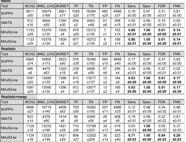
2.4.2. Comparison between methods on synthetic data
The dataset from Keane et al. (2011) was used as input for simulating RNA-seq experiments
using BEERS. The resulting FASTA files were quantified for differential splicing between
simulated hippocampus and liver using SUPPA, rMATS, and MAJIQ with and without
local-weights outlier correction. Events were called as significantly-changing based on the
recommendations of the tools’ respective authors. These results are depicted in Figure 8.
The definition of what constitutes a splicing event depends on the tool in use, and the total
number of events quantified (the sum of the #CHG, #NO CHG, and #GREY columns)
reflects this. SUPPA, for instance, attempts to quantify Ψ for all annotated binary events.
rMATS, meanwhile, only considers splicing events that fit a limited model of local splicing
variations. MAJIQ, meanwhile, is the only tool out of the three that attempts to quantify
more complex splicing variations, though its event count is slightly lower than that of
SUPPA due to the stringent quantifiability filters MAJIQ imposes. In MAJIQ’s case, when
a splicing event is ambiguously described by two or more LSVs, the ambiguity is resolved
by taking the LSV reporting the highest P(|∆Ψ| ≥20%). Based on the observations from Section 2.4.1, we perform all further comparative analyses on only the MAJIQ-nw and
MAJIQ-lw models.
For each algorithm, we counted the number of splicing events reported as not changing
d e f
g h i
a b c
(𝜃) (𝜃) (𝜃)
(𝛿) (𝛿) (𝛿)
(𝛾) (𝛾) (𝛾)
Figure 7: Synthetic perturbation of tissue replicates. In each test, three cerebella were com-pared against three livers from Zhang et al. (2014), but one of the cerebella was perturbed. MAJIQ-nw is the previous algorithm equivalent to fixed weights (ρt = 1). MAJIQ-rm is
a control case where we assume some heuristic (e.g. PCA) was able to detect the outlier and remove it before executing the previous fixed-weights MAJIQ. a,d,g. Effect on ρt for
the perturbed “outlier” (blue) and unperturbed replicates (Rep1,2 in green and orange).
b,e,h. Effect on the numberNA of events detected to have P(∆Ψ>0.20)>0.95 between