Vol 9, No 3 (2018)

International Journal of Mathematical Archive-9(3), 2018,

Available online throug

International Journal of Mathematical Archive- 9(3), March – 2018 52 CONFERENCE PAPER

National Conference dated 26th _{Feb. 2018, on “New Trends in Mathematical Modelling” (NTMM - 2018),}

Organized by Sri Sarada College for Women, Salem, Tamil Nadu, India.

EXPLORATION OF MATHEMATICAL MODELLING IN DATA MINING

M. KANIMOZHI

Ph.D. Research Scholar (Computer Science)

Sri Sarada College for Women (Autonomous), Salem-16, India.

R. ROSELIN

Associate professor of Computer Science,

Sri Sarada College for Women (Autonomous), Salem16, India.

E-mailan

ABSTRACT

Data plays a potential role in making decision. This data can be mined to get some useful information. Here

Keywords: Data Mining, Mathematical Modelling, breast cancer data set.

1. INTRODUCTION

Data mining is defined as extracting of knowledge from huge amount of data. Data mining involves the raw data, data management system, data pre-processing aspects and finding the pattern within the large amount of unexploring database. There are many other terms carrying a similar or a little different meaning to Data mining, such as knowledge mining from databases, knowledge extraction, data pattern analysis, data archaeology and data dredging. Data Mining is one of the steps in Knowledge Discovery in Databases (KDD). KDD and is defined as the nontrivial process of identifying valid, novel, potentially useful and ultimately understandable patterns of interest in data [7]. Data mining pre-processing steps include the filling the missing value, removing the noisy data.The data collection instruments used may be faulty. There may have been human or computer errors occurring at data entry. Users may purposely submit incorrect data values for mandatory fields when they do not wish to submit personal informationdata.Discretization which converts continuous values into discretized one, normalization which is used to scale the data and mapping the data. Normalization technique is used to find the new value from the existing data and required make them closer.

Figure-1: Overall Process

Mathematical models play an important role in identifying the pattern [2] [6]. This paper is organized as follows: Section 1 introduces the concept, Data set description is given in section 2, Data cleaning is discussed in Section 3, Section 4 discusses the process of feature selection with respect to quick reduct algorithm, Section 5 describes the classification models, Experimental results are discussed in Section 6 and Section 7 concludes this with the perspective to further research.

2. DATA SET DESCRIPTION

Breast Cancer Wisconsin (Original) data Set is taken from UCI data repository. It has 699 instances, 10 attributes and it also has missing values. The following are the attribute information:

1. Sample code number (F1) :id number 2. Clump Thickness (F2) : 1 - 10 3. Uniformity of Cell Size (F3) : 1 - 10

4. Uniformity of Cell Shape (F4) : 1 - 10 5. Marginal Adhesion (F5) : 1 - 10

6. Single Epithelial Cell Size (F6) : 1 - 10 7. Bare Nuclei (F7) : 1 - 10 8. Bland Chromatin (F8) : 1 - 10 9. Normal Nucleoli (F9) : 1 - 10 10. Mitoses (F10) : 1 - 10

11. Class : (2 for benign, 4 for malignant)

missing values are represented by ’?’. Sample instances from breast cancer data set are given in Table 1.

Table-1: Breast Cancer Data Instances (Sample)

F1 F2 F3 F4 F5 F6 F7 F8 F9 F10 Class 1183246 1 1 1 1 1 ? 2 1 1 2 1183516 3 1 1 1 2 1 1 1 1 2 1183911 2 1 1 1 2 1 1 1 1 2 1183983 9 5 5 4 4 5 4 3 3 4 1184184 1 1 1 1 2 5 1 1 1 2 1184241 2 1 1 1 2 1 2 1 1 2 1184840 1 1 3 1 2 ? 2 1 1 2 1185609 3 4 5 2 6 8 4 1 1 4

3. DATA PRE-PROCESSING

This is the important step in data mining. Raw data are needed to be cleaned before mining because it may contain noise. Some of the data may be inconsistent.

3.1 Data cleaning

This process removes noisy and inconsistent data from breast cancer data set

3.2 Smoothing

For smoothing the data, binning technique can be used. Binning methods smooth data value by considering its “neighborhood”. The sorted values are distributed into a numberof “buckets” orbins. Smoothing can be done by mean, median and boundaries.

Data Acquisition

Pre-Processing (Missing Values,

Di ti ti N li ti )

Feature Selection (Rough based Quick Reduct)

Classification (Naive Bayes,J48,JRip)

3.3 Outliers

A data set may contain objects that do not realize the general behavior or model of the data. These data are outliers. Many data mining methods reject outliers as noise or exceptions. Outliers may be detected and handled using statistical tests.This assumes a distribution or probability model for the data, or by using distance measures identify the outliers [7].

3.4 Missing values

Data are not always available incomplete form in real data set. It may be incomplete and noisy.Some tools ignore missing values; others use some metric to fill in replacements. The metric are:

i. Ignore the tuple.

ii. Fill in the missing value manually.

iii. Use a global constant to fill in the missing value. iv. Use the attribute mean or median.

v. Use the attribute mean or median for all samples belonging to the same class as the given tuple. vi. Use the most probable value to fill in the missing value.

To fill the missing value, the mean and median values are used for data replacement. The breast cancer data set has16missing values as ‘NaN’. In this study mean value is computed to replace the missing values [8].

Mean (𝑋�)=∑ 𝑋𝑖 𝑛 𝑛 𝑖=1

Figure 2 shows the Missing values replaced by mean.

Figure-2: Missing Values Replaced by Mean

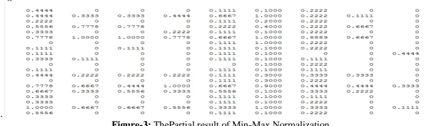
3.5 Min-Max Normalization

Data set can also be in varying from, e.g. one attribute varies in range of 100 and other attribute varies in the range of 10000. So, a proper normalization of data set is done in which each attribute come in the range of 100 or whatever user selects. This normalization technique is known as Min-max normalization.

B = ( (A−minimumvalueofA)

(maximumvalueofA−minimumvalueofA)) *(D-C)

The min-max normalization is pre-processing techniques to scale the data in the range of −1.0 to 1.0, or 0.0 to 1.0.The above formula applying for the min-max function then the original data convert the scale 0 to 1.

.

Figure-3: ThePartial result of Min-Max Normalization

3.6 Discretization

3.7 Rough Set based Feature Selection

Feature selection refers to the process of selecting those input attributes that are most predictive of a given outcome. Unlike other dimensionality reduction methods, feature selectors preserve the original meaning of the features after reduction. Rough set theory (RST) can be used as tool to discover data dependencies and reduce the number of attributes contained in data set using the data along, requiring no additional information [5]. It is possible to find the set of the original attribute using RST that are most informative, all other attributes can be removed from the data set with minimal information loss. The benefits of feature selection are twofold: it considerably decreases the running time of the induction algorithm, and increases the accuracy of the resulting model.

4. QUICK REDUCT ALGORITHM

The quick reduct algorithm is used to calculate a reduct without considering all possible subsets. It starts up with an empty set and adds in turn, one at a timethose attribute result ingreatest increase in the rough set dependency metric, until this process maximum possible value for dataset. This algorithm calculated the dependency for each attribute and chooses the best candidate.

4.1 Reduct

Reduct is a minimal subset R of initial attribute set C(conditional) such that for a given set of decision attribute D [1]. Quick reduct algorithm reduced 10 attributes of breast cancer data set into 4 attributes. Id is removed before applying quick reduct algorithm. They are Clump Thickness (F2), Uniformity of Cell Size (F3), Bare Nuclei (F7) and Normal Nucleoli (F9).

5. CLASSIFICATION

Data classificationis a two-step process, consisting of a learning step and a classification step. In the first step, a classifier is built describing a pre-determined set of data classes or concepts. There aremany classification algorithms. This paper deals only with the following:

i. Decision tree classification ii. Bayesian classification iii. Rule based classification

5.1 Naive Bayes Classification

Naive Bayes model is probability based model. It uses prior probability. The method is simple and easy to build. Bayes theorem provides a way of calculating posterior probability, P(C|x), from P(C), P(x) and P(x|C).

5.2 J48 classification

Information gain is the measure used in building a decision tree. The table is split based on the information gain. Leaf nodes bear the class value when the splitting procedure stops if all instances in a subset belong to the same class.The model generated by J48 is given below:

5.3 Rule based JRip Algorithm

JRip (RIPPER) is one of famous algorithms has its own popularity. Incremental reduced error is used to generate set of rules for the class.

Figure-5: JRip Classifier

6. EXPERIMENTAL RESULTS

Pre-processing is done using MATLAB and the classification is done in WEKA. Table 2 reports the validation measures as per classifier.

Table-2: Validation Measures

Classification Before QR After QR Before QR After QR Precision Recall Precision Recall Naivebaye (436,235) (441,237) 0.962 0.960 0.971 0.970 J48 (44,225) (439,227) 0.956 0.956 0.953 0.953 JRip (438,232) (441,231) 0.959 0.959 0.962 0.961

The experimental results before and after quick reduct algorithm is illustrated in Figure 6. The experimental result shows that classification produces good result after feature selection for breast cancer data set.

Figure-6: Comparative study of Precision and Recall

7. CONCLUSION

8. REFERENCE

1. Anitha K., Venkatesan P., “Feature Selection by Rough-Quick Reduct Algorithm”, International Journal of Innovative Research in Science, Engineering and Technology, Vol. 2, pp. 3989-3993, 2013.

2. Elmegård Michael, Starke Jens, “Mathematical Modeling and Dimension Reduction in Dynamical Systems”, Ph. D. Thesis, Technical University of Denmark, ISSN 0909-3192, 2014.

3. KeerthikaT., Premalatha K., “Rough Set Reduct Algorithm based Feature Selection for Medical domain”, Journal of Chemical and Pharmaceutical Sciences, Vol. 9, Issue 2,pp. 896-902, 2016.

4. Mario Rosario Guarracino, “On Classification Methods for Mathematical Models of Learning”,High Performance Computing and Networking Institute Italian National Research Council, pp. 2-12, 2005.

5. Pawlak Z, “Rough Sets”, International Journal of Computer and InformationSciences, Vol. 11, No. 5, pp. 341–356. 1982.

6. Suresh G., Selvakumar I.A., “An Overview of Data Mining Concepts Applied in Mathematical Techniques”, International Journal of Computing Algorithm, Vol. 3, pp. 905-909, 2014.

7. “Data Preparation for Data Mining”, Dorian Pyle, 1999.

8. “Data Mining: Concepts and Technique”, JiaweiHan and Micheline Kamber, 2000.