INTRODUCTION
Anthropogenic activities are having a major effect on the marine ecosystem. The ongoing global release of greenhouse gases and subsequent warming has forced ocean temperature to rise at a rate of ~0.4°C over the last century (Rayner et al. 2003). The planet as a whole is currently experiencing the warmest period over the past 100 yr, and a 2 to 4.5°C rise in
land and ocean temperature is predicted by the end of this century (IPCC 2007). This change could have profound impacts on phytoplankton in terms of com-munity structure, physiology and primary production (Hughes 2000, Atkinson et al. 2003, Fu et al. 2007, Feng et al. 2009, Boyd et al. 2010). Data from the continuous plankton recorder (CPR) survey in the northeast Atlantic have shown that rising sea surface temperature (SST) has increased phytoplankton
*Corresponding author: [email protected]
Effect of increases in temperature and
nutrients on phytoplankton community structure
and photosynthesis in the western English Channel
Yuyuan Xie
1, 2, Gavin H. Tilstone
1,*, Claire Widdicombe
1, E. Malcolm S. Woodward
1,
Carolyn Harris
1, Morvan K. Barnes
1, 3 1Plymouth Marine Laboratory, Prospect Place, Plymouth PL1 3DH, UK2Present address: College of Environment and Ecology, Xiamen University, Xiamen 361005, PR China 3Present address: CNRS, Laboratoire d’Oceanographie de Villefranche, Villefranche-sur-Mer, France
ABSTRACT: Anthropogenic climate change is exerting pressures on coastal ecosystems through increases in temperature, precipitation and ocean acidification. Phytoplankton community structure and photo-physiology are therefore adapting to these conditions. Changes in phyto-plankton biomass and photosynthesis in relation to temperature and nutrient concentrations were assessed using a 14 yr dataset from a coastal station in the western English Channel (WEC). Dino-flagellate and coccolithophorid biomass exhibited a positive correlation with temperature, reaching the highest biomass between 15 and 17°C. Diatoms showed a negative correlation with tempera-ture, with highest biomass at 10°C. Chlorophyll a(chl a)normalised maximum light-saturated pho-tosynthetic rates (PB
m) exhibited a hyperbolic response to increasing temperature, with an initial linear increase from 8 to 11°C and reaching a plateau from 12°C. There was, however, no significant positive correlation between nutrients and phytoplankton biomass or PB
m, which reflects the lag time between nutrient input and phytoplankton growth at this coastal site. The ma-jor phytoplankton groups that occurred at this site occupied distinct thermal niches, which in turn modified PB
m. Increasing temperature and higher water column stratification were major factors in the initiation of dinoflagellate blooms at this site. Dinoflagellate blooms during summer also co-varied with silicate concentration and acted as a tracer of dissolved inorganic nitrogen and phos-phate from river run-off, which were subsequently reduced during these blooms. The data imply that increasing temperature and high river runoff during summer will promote dinoflagellate blooms in the WEC.
KEY WORDS: Temperature · Nutrients · Eutrophication · Phytoplankton community structure · Photosynthesis · Western English Channel
O
PEN
PEN
A
CCESS
CCESS
© The authors 2015. Open Access under Creative Commons by Attribution Licence. Use, distribution and reproduction are un -restricted. Authors and original publication must be credited. Publisher: Inter-Research · www.int-res.com
abundance in cooler regions but decreased it in warmer regions (Richardson & Schoeman 2004). Over the past 100 yr, the western English Channel (WEC) has experienced a sequence of warming and cooling events which have caused changes in the abundance of marine phytoplankton. A 1°C rise in SST for a decade during the 1990s caused an increase in warm-water species in this region (Hawkins et al. 2003). In the WEC over the past 15 yr from 1992 to 2007, there was a decrease in diatoms
and Phaeocystis sp. and an increase in
dinoflagel-lates and coccolithophorids (Widdicombe et al. 2010). Against the backdrop of global warming in Euro-pean waters, eutrophication has been a major prob-lem for the coastal zone and has resulted in large and sometimes harmful phytoplankton blooms that can cause hypoxia or toxicity (Nixon 1995, Harley et al. 2006, Rabalais et al. 2009). In Europe, the North Sea, Baltic Sea and eastern English Channel are hotspots for eutrophication that have been linked to more fre-quent blooms of nuisance species, such as
Phaeocys-tis globosa(Lancelot et al. 1987, Riegman et al. 1992,
Schoemann et al. 2005). The EU Water Framework Directive was implemented to curb these effects, although regime shifts in the phytoplankton have still occurred, which have been linked to the rise in SST (McQuatters-Gollop et al. 2007b). Associated with this, changes in the jet stream arising from small latitudinal temperature gradients have led to more frequent storm events and heavy rainfall, which have intensified over the past decade (Rahmstorf & Coumou 2011, Francis & Vavrus 2012). Recent cli-mate modelling also predicts an increase in annual rainfall coupled with the rise in temperature across much of the United Kingdom by the end of this cen-tury (Jenkins et al. 2009). Localised flooding in the catchment around the WEC in the summer of 2007 led to an increase in chlorophyll a (chl a)of 8.46 µg l−1 at in-shore stations due to high nutrient loads from river run-off (Rees et al. 2009).
It is often difficult to de-couple temperature and nutrient effects in marine environments, as they are intrinsically linked. In this study, we investigated the effects of variability in temperature, nitrate, phos-phate and silicate concentrations on phytoplankton community structure and photosynthesis in the WEC. We analysed medium term trends (~14 yr) in the taxonomic biomass and photosynthetic response of phytoplankton to variations in temperature and nutrients. The results are discussed in relation to the underlying mechanism of seasonal succession in phytoplankton community and photosynthesis and the implication of future environmental changes.
MATERIALS AND METHODS Study site and sampling
Stn L4 (50° 15’ N, 4° 13’ W) is situated in the WEC, 15 km southwest of Plymouth, England, with a depth of ca. 50 m (Fig. 1). Sampling at the site has been established for over a century, and a long-term obser-vation on a weekly basis was initiated with profiles of temperature, salinity and fluorescence in 1988. Measurements of phytoplankton counts and chl a
were added in 1992, nutrients in 2000, and primary production in 2009 (Southward et al. 2004, Smyth et al. 2010). Samples were collected using a Lagrangian sampling mode whereby the ship is allowed to drift with the sampled water body once the sampling loca-tion has been reached. The tide at the site has a max-imum range of 5.4 m and a current of 0.55 m s−1 (Pin-gree 1980). The river Tamar is the main source of freshwater flowing into the WEC, with a range of 5 to 140 m3 s−1 at its mouth (Uncles & Stephens 1990). Vertical profiles of temperature, salinity and fluores-cence have been measured using SeaBird SBE19+
Fig. 1. Location (50° 15’ N, 4° 13’ W) of Stn L4 in the western English Channel. R: river
CTD since 2002. Water samples were collected in discrete sampling bottles or carboys and returned to the laboratory in black-out cool-boxes within 2 h of collection for measurement of the parameters given below. The mixed layer depth (MLD) when the den-sity difference is < 0.125 kg m−4from the surface was used. Meteorological measurements including wind speed, wind direction and rainfall have been taken at hourly intervals from the roof of Plymouth Marine Laboratory since 2003 (Smyth et al. 2010).
Nutrients, chl aand taxonomic phytoplankton
biomass
Dissolved inorganic nutrient concentrations were determined by gas segmented flow colorimetric analysis using a Bran and Luebbe AutoAnalyser (model AA3). Dissolved NO3−+ NO2− were deter-mined by the spectrophotometric methods described by Brewer & Riley (1965). Total ammonium was determined according to Mantoura & Woodward (1983). The analysis of soluble reactive phosphorus (SRP) concentration was based on the method de -scribed by Zhang & Chi (2002). Dissolved silicate (DSi) was determined using standard colorimetric methods (Kirkwood 1989). Seawater samples were collected directly from the CTD rosette, stored frozen until analysis and then equilibrated to room temper-ature prior to analysis, following the protocols given in the GO_SHIP manual (Hydes et al. 2010). Dis-solved inorganic nitrogen (DIN) was calculated from the sum of the concentration of NO3−+ NO2− and ammonium.
Fluorometric analysis of chl awas conducted using 100 ml of seawater filtered through 25 mm (nominal pore size ~0.7 µm) glass-fibre filters (GF/F) and extracted in 90% acetone overnight at 4°C. Chl a
concentration was then measured on a Turner fluo-rometer using the Welschmeyer (1994) method.
Samples for the enumeration of phytoplankton were fixed immediately on collection with 2% Lugol’s iodine and stored in cool, dark conditions until taxonomical analysis using light microscopy following the methods given by Widdicombe et al. (2010). Cell volumes were calculated using approxi-mate geometric shapes and converted to carbon biomass using the equations of Menden-Deuer & Lessard (2000). The data are plotted as 4 phytoplank-ton groups: diatoms, coccolithophorids, dinoflagel-lates and nano-eukaryotes. The dynamics in biomass of key species within some groups were also inves -tigated.
Phytoplankton photosynthetic parameters
Phytoplankton photosynthetic parameters were calculated from photosynthesis-irradiance (P-E)curves measured using linear photosynthetrons illuminated with 50 W tungsten halogen lamps following the methods described by Tilstone et al. (2003). For each depth, 15 aliquots of 70 ml seawater within polycar-bonate bottles (Nalgene) were inoculated with 5 to 10 µCi of 14C-labelled bicarbonate. Incubations were maintained at in situtemperature for a 1.5 h period, after which the samples were filtered onto GF/F under a vacuum pressure no greater than 27 kPa. The filters were then exposed to 37% fuming hydro -chloric acid for ~12 h and immersed in 4 ml scintilla-tion cocktail for 24 h, and beta-activity was counted on a TriCarb 2910 scintillation counter (PerkinElmer). Correction for quenching was performed using the external standard and the channel ratio methods. Total inorganic carbon fixation within each sample was calculated following Tilstone et al. (2003) and normalized to chl a, and the curves were then fitted using the equation given by Platt et al. (1980):
PB = PB
s[1 − exp(−αI/PBs)] exp(−βI/PBs) (1) where PB
s is the potential light-saturated photosyn-thetic rate the sample could have if there was no photoinhibition, αis the light-limited slope, βis the parameter representing the reduction by photoinhi-bition, and Iis irradiance. The maximum photosyn-thetic rate (PB
m) is calculated as follows:
PB
m = PBs[α/(α + β)] [β/(α + β)]β/α (2)
Statistical analysis
Time series data from Stn L4 at 10 m between April and September from 2000 to 2013 were used to assess the effect of natural variability in nutrients and temperature on phytoplankton community biomass and photosynthesis. Data from winter months were not used since nutrients are always high and phyto-plankton biomass low during these months, which is forced by reduced PAR. Including the winter data would therefore skew any subsequent relationships between nutrients and phytoplankton biomass. Nutrient data at 10 m was only available from 2012; prior to this, nutrients were measured at the surface only. We therefore assumed that the upper mixed layer was uniform from the surface to 10 m and used the surface values prior to 2012. Chl aat 10 m was available from 2007 to 2013. Prior to 2007, chl aat
10 m was calculated from surface chl a using the equation log10Chl(10)= 0.9359 × log10Chl(0)+ 0.002 (n = 215, R2 = 0.845) based on the data from successive years. Coincident with temperature and nutrient data, there were n = 235 data for chl a, n = 222 for biomass of phytoplankton groups and n = 68 for PB
m.
These data are presented as box and whisker plots at 1°C increments in temperature and logarithmic increments of nutrient concentrations. The height of the box indicates the 25th (Q1) and 75th (Q3) per-centiles; the horizontal line and solid circle inside the box are median and mean, respectively. The whisker limits are defined as Q3 + (1.5 × interquartile range, IRQ) and Q1 − 1.5 × IRQ and represent the 10th and 90th percentiles. The outliers outside of the whiskers are given as open circles. Correlation between 2 vari-ables using the exact temperature and nutrient data (rather than the binned data) was determined by Spearman’s non-parametric rank correlation coeffi-cient in R software (R Development Core Team 2013). To avoid increasing a Type I error through the repetition of analyses, the following procedure was conducted: when p is the Type I error, (1 − p) repre-sents the rate of not making Type I error, the product of (1 − p) is the rate of not making Type I error for all tests. Routinely, the value with the highest Type I error is removed until the product of (1 − p) meet the criterion of > 0.95 (and p < 0.05), > 0.99 (p < 0.01) and > 0.999 (p < 0.001) successively. Thus, in the text, the corrected p values are reported. The logit regression was employed to examine the possibility of dominant species forming blooms (with a bloom criterion of >10 mg C m−3). Temperature (T ), DIN, SRP and DSi were used as predictors, and the interaction term was used to evaluate combined affects with bloom possi-bilities derived as follows:
F (t) = F (T,DIN,SRP,DSi)
= 1/
[
1 − exp(−β0− β1T− β2DIN − β3SRP − β4DSi − β5T× DIN − β6T× SRP − β7T× DSi)]
(3)F (t)is the logit regression function with t as the linear combination of predictors. The results of F (t)range between 0 and 1, representing the probability for a bloom to occur. Forward selection was used based on Akaike’s information criterion (AIC) by stepwise pro-cedure in R software (R Development Core Team 2013) to obtain the best predictive model. The signif-icance of each coefficient (βx) was determined, and the significance of the whole model was determined using a chi-squared distribution. The possibility of a bloom for the species above was predicted in each temperature interval by using average values of binned DIN, SRP and DSi as inputs.
RESULTS
Natural variability in chl a, phytoplankton biomass
and PB
min relation to temperature and nutrients
in the WEC
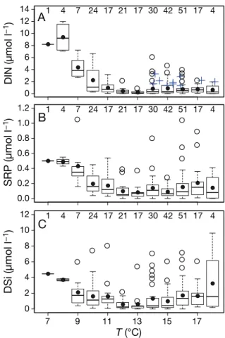
Between April and September 2000 to 2013, tem-perature varied from 7.3 to 18.2°C with the highest temperature in mid-August. During this period, ~20% of DIN was < 0.1 µmol l−1, and ~30% was >1 µmol l−1(Fig. 2A). There was a negative inverse relationship between temperature and DIN and SRP from 7 to 11°C, beyond which there was no obvious relationship, except for a slight increase in SRP from 16 to 18°C (Fig. 2A,B). Spikes in DIN during July and August at between 14 and 18°C also occurred,
DIN (µmol l
−1
)
0 2 4 6 8 10 12
14 1 4 7 24 17 21 17 30 42 51 17 4
A
SRP (µmol
l
−1
)
0.0 0.2 0.4 0.6 0.8 1.0
1.2 1 4 7 24 17 21 17 30 42 51 17 4
B
T (°C)
DSi (µmol
l
−1
)
7 9 11 13 15 17
0 2 4 6 8 10
12 1 4 7 24 17 21 17 30 42 51 17 4
C
● ●
● ● ● ● ●●
● ● ● ●
●
●
●
● ● ●
●
● ● ● ●
● ●
● ● ●
● ●
●
● ●
● ● ● ● ●
● ●
● ● ● ●
● ●
● ●
● ●
● ● ● ● ● ●
● ●
●
● ●
● ● ● ● ●
● ●
● ●
● ● ●
● ● ● ●
● ●
●
Fig. 2. Concentrations of (A) dissolved inorganic nitrogen (DIN), (B) soluble reactive phosphorus (SRP) and (C) dis-solved silicate (DSi) as functions of temperature (T ) from April to September 2000–2013 at Stn L4 in the western Eng-lish Channel. For the box plots, the boundaries of the boxes represent the 25th and 75th percentile; the solid line within the box is the median; the black dot is the mean; the error bars above and below the box indicate the 10th and 90th percentiles, and the points beyond the error bars are the out-liers. Number of samples in discrete Tranges is given at the top of each panel. In (A), blue crosses indicate spikes in
though these do not adversely affect the binned median or mean values. For the low temperature range (7 to 9°C), DSi was low relative to DIN, and the average ratio of DSi to DIN was lower than Brzezin-ski’s ratio (molar ratio of 1). At the upper limit of the temperature range (16 to 18°C), the mean DSi con-centration was >1.5 µmol l−1, and the average ratio of DSi to DIN was > 2; at 18°C, this reached a molar ratio of 5 (Fig. 2C). There was no significant correlation between chl a(p > 0.05; Fig. 3A) or total phytoplank-ton biomass and temperature (p > 0.05; Fig. 3B). The distribution of the binned values of both chl a and total phytoplankton biomass were bimodal, illustrat-ing the occurrence of 2 blooms. The first occurred in spring, between 9 and 12°C. The second was in summer at temperatures of between 14 and 17°C (Fig. 3B). Numerically, diatoms and nano-eukaryotes were the most abundant groups and contributed, on average 38 and 37% of the total phytoplankton bio-mass. By comparison, dinoflagellates and coccolitho-phorids contri buted 22 and 5%, respectively. These group contributions to the total biomass changed over different temperature ranges (Fig. 4E). Dinofla-gellates, for example, formed 28% of total phyto-plankton biomass from 14 to 18°C (Fig. 4E), though this occasionally rose to > 50% and very occasionally to > 90%. At the same temperature range, the aver-age percentaver-age of nano- eukaryotes and diatoms dropped to 66 from 91% at lower temperatures (Fig. 4E). Over the entire temperature range for nano-eukaryotes, there was no sig nificant correlation with temperature (p > 0.05; Fig. 4A). In contrast, there were positive linear correlations for both coccolitho-phorids (p < 0.001; Fig. 4C) and dinoflagellates (p <
0.001; Fig. 4D), and there was a negative correlation with diatoms (p < 0.05; Fig. 4B). The contributions of diatoms to total phytoplankton biomass were higher during the spring bloom, but de creased with temper-ature (p < 0.01; Fig. 4E). In contrast, there was a sig-nificant positive correlation between the percentage of dinoflagellates and temperature, with the propor-tion of dinoflagellates increasing with in creasing temperature (p < 0.001, Fig. 4E).
PB
mvaried from 0.2 to 7.5 mg C mg chl a−1h−1and exhibited a positive linear correlation with tempera-ture from 9 to 11°C and thereafter remained rela-tively constant from 12 to 17°C with a mean value of ~4 mg C mg chl a−1h−1(Fig. 5A). The trend in PB
m with temperature could be explained by a hyperbolic function, as follows:
PB
m = 3.77tanh[0.46(T− 8)] (4) where Tis temperature, and R2= 0.112. There were no significant correlations between chl a(p > 0.05; Fig. 3C) or total phytoplankton biomass and nutrients (p > 0.05; Fig. 3D). When there were spikes in DIN from July to August, both chl aand total phytoplank-ton biomass varied from the lowest to the highest val-ues in the binned data (Fig. 3A,B). Dinoflagellates exhibited a significant negative correlation with DIN (p < 0.001; Fig. 6A). Diatoms showed negative corre-lations with SRP and DSi (p < 0.01 and p < 0.001, respectively; Fig. 6B,C). Coccolithophorid biomass was significantly positively correlated with DSi (p < 0.05; Fig. 6D). Over the entire nutrient range, there was also no significant correlation between PB
mand
DIN (p > 0.05; Fig. 5B) as well as SRP (p > 0.05; data not shown) and DSi (p > 0.05; data not shown). ●
● ● ●
● ●
● ● ●
Chl
a
(mg m
−3
)
1
●
4
●
7
●
24
●
17
●
21
●
17
●
30
●
42
●
51
●
17
●
4
●
A
● ●
● ● ●
● ●
●
0 2 4 6 8 10 12 45
●
36
●
90
●
38
●
26
●
C
●
● ● ●● ●
● ●
●
7 9 11 13 15 17
T (°C)
T
otal phytoplankton
(mg C m
−3
)
2
●
7
●
16
●
20
●
15
●
18
●
31
●
43
●
49
●
16
●
5
●
B
●
● ● ● ●
● ●
< 0.1
0.1−0.30.3−1 1−3
> 3
10 102 103
0 2 4 6 8 10 12
10 102 103
DIN (µmol l−1)
43
●
40
●
84
●
34
●
21
●
D
Fig. 3. (A) Chlorophyll a (chl a) and (B) total phytoplankton biomass as a function of temperature (T ). (C) Chl aand (D) total phytoplankton biomass as a function of dissolved inorganic nitrogen (DIN) from April to September 2000 to 2013 at Stn L4 in the western English Channel. Number for the discrete T and DIN ranges are given at the top of each panel. Blue crosses in (A) and (B) represent the bio-mass of the DIN spikes in Fig. 2A; see
Logit regressions of phytoplankton bloom occurrences
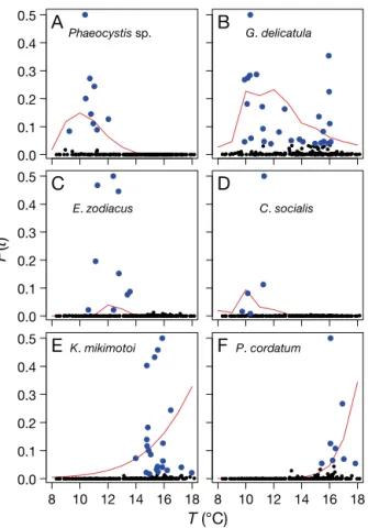
From 2000 to 2013 in the WEC, Phaeocystis sp. accounted for 12.6% of the nano-eukaryote biomass and tended to bloom when the temperature was <12°C (Fig. 7A, Table 1). Guinardia delicatula,
Eu-campia zodiacus and Chaetoceros socialis were the
most abundant diatoms and accounted for 16.3, 12.4
and 10.8% of the total diatom biomass, respectively. For these species, temperature exhibited a significant inverse relationship with biomass > 10 mg C m−3 (Table 1). G. delicatulaexhibited a larger temperature range (10 to 16°C) during bloom conditions and a higher frequency of bloom events (Fig. 7B). In con-trast, E. zodiacushad a narrower and lower tempera-ture range (10 to 14°C) (Fig. 7C). This was even lower for C. socialis(<12°C; Fig. 7D). SRP showed a consis-●
● ● ● ● ●
●
●
1 10 102
2
●
7
●
16
●
20
●
15
●
18
●
31
●
43
●
49
●
16
●
5
●
A
●
●
2
●
7
●
16
●
20
●
15
●
18
●
31
●
43
●
49
●
16
●
5
●
C
● ●
●
● ●
7 9 11 13 15 17
10−2 10−1 1 10 102
103
1 10 102
10−2 10−1 10−2 10−1
1 10 102
103
2
●
7
●
16
●
20
●
15
●
18
●
31
●
43
●
49
●
16
●
5
●
B
● ●
● ●
● ●
7 9 11 13 15 17
2
●
7
●
16
●
20
●
15
●
18
●
31
●
43
●
49
●
16
●
5
●
D
Biomass (mg C m
−3
)
T (°C)
T (°C)
Change (%)
7 9 11 13 15 17
0 20 40 60 80 100
E
DinoflagellatesCoccolithophorids Diatoms
Nano-eukaryotes
Fig. 4. Relationship between carbon biomass of (A) nano-eukaryotes, (B) diatoms, (C) coccolithophorids and (D) dinoflagellates and temperature (T )from April to September, 2000–2013, at Stn L4 in the western English Channel. Number in discrete Tranges is given at the top of each panel. Linear regression lines (solid) are given in panels: (B) log10(Biomass) = −0.048T +
1.654 (R2= 0.02, p < 0.05); (C) log
10(Biomass) = 0.142T−
2.468 (R2= 0.13, p < 0.001); (D) log
10(Biomass) = 0.225T
− 2.711 (R2= 0.33, p < 0.001). (E) Percentage change in
phytoplankton groups to total biomass in relation to temperature. See Fig. 2 for box plot information
9 11 13 15 17
0 2 4 6 8 10
P
B m
(mg C mg
−1
chl
a
h
−1
) 3 9 5 7 6 4 15 12 3
A
T (°C)
0.1 0.3 1 3
0 2 4 6 8 10
DIN (µmol l−1)
14 15 20 8 7
B
Fig. 5. (A) Chlorophyll a normal-ized light-saturated photosyn-thetic rate (PB
m) in relation to
temperature (T )and (B) in rela-tion to dissolved inorganic nitro-gen (DIN) from April to Septem-ber, 2000–2013, at Stn L4 in the western English Channel. The dashed line is the hyperbolic curve fit. See Fig. 2 for box plot
tent significant negative effect on possible bloom oc-currences (Table 1), indicative of the reduction in SRP during bloom events. More than half of the dinoflagel-late biomass (59.2%) during the time series was from
Karenia mikimotoi, whilst Prorocentrum cordatum
ac-counted for 7.5%. Dinoflagellate blooms tended to oc-cur when temperature was >14°C. For P. cordatum, this temperature threshold was 16°C (Fig. 7E,F), and increasing DIN also had a positive effect (Table 1).
Emiliana huxleyi biomass rarely reached 10 mg C
m−3, and there was no single environmental variable that was significant in the logit regression (Table 1). ● ● ● ● ● ● ● ● ● ● ●
0.1 0.3 1 3
43 ● 40 ● 84 ● 34 ● 21 ●
A
DIN ● ● ● ● ● ● ● ●0.1 0.3 1 3
22 ● 39 ● 58 ● 72 ● 31 ●
C
DSi ● ● ● ● ● ● ● ●0.03 0.1 0.3 30 ● 75 ● 82 ● 35 ●
B
SRP0.1 0.3 1 3
10−2 10−1 1 10 102 103 10−2 10−1 1 10 102 103 10−2 10−1 1 10 102 103 10−2 10−1 1 10 102 103 22 ● 39 ● 58 ● 72 ● 31 ●
D
DSiBiomass (mg C m
−3
)
Fig. 6. Relationship between carbon biomass of (A) dinofla-gellates and dissolved inorganic nitrogen (DIN), (B) diatoms and soluble reactive phosphate (SRP), (C) diatoms and dis-solved silicate (DSi), (D) coccolithophorids and DSi from April to September, 2000–2013, at Stn L4 in the western English Channel. Number in discrete DIN ranges is given at
the top of each panel. See Fig. 2 for box plot information
0.0 0.1 0.2 0.3 0.4 0.5 ●● ● ●●●●●●● ●●●●●●●● ●●●●●●● ●●●●●●● ●●●●●●●●●●●●●●●●● ●●●●●●●●●●●●●●●●●●●●●●●●●●●●●●● ●●●●●●●● ●●●●●●●●●●●●●●●●● ● ●● ●●●●● ●●●●●● ● ●● ●● ●●● ●●● ● ●●●●●●●●●●● ● ● ●●● ●● ●●●● ● ●●●●● ●●●●●●●●● ●●● ●●●●●●●●●●●●●●● ●●●●●● ●●●●●●● ●●●●●●●●●●●●●● ● ● ● ● ● ● ● ● ●
A
Phaeocystis sp.
● ● ● ● ● ●● ●●●●●●●● ●● ●● ●● ●●●●●●●● ●●●●● ● ● ● ●●●●● ●●●●● ●●●●●● ●●●●●●●●●●●●●●●●●●●●●●●●●●●●●●●●●●●●● ● ● ● ● ● ●● ● ●● ● ●●●● ●● ● ●● ● ● ●● ●●●●●● ●●●●●●●● ●●●●● ●●●●●●●● ●●● ● ● ● ● ●●● ●●●●● ● ●●● ●● ● ●● ● ● ● ● ● ● ● ●●●● ● ●●●● ● ● ● ●● ● ● ●●● ●● ●● ● ● ● ● ● ● ● ●● ● ● ● ● ●● ● ● ● ● ● ● ● ● ● ● ● ●
B
G. delicatula
0.0 0.1 0.2 0.3 0.4 0.5 F ( t ) ●● ●● ●●●●● ●●●●●●● ●●●●●●●● ●●●●●●●●●● ●●●●●● ●●●●●●●●●●●●●●● ●●●●●●●●●●●●●●●●●●●●●●●●●●●●●●●● ●●●●●●●● ●●●●●●●●●●●●●●●●● ● ●●●●●● ●●●●●● ● ●●● ●● ●●●●●● ●●●●●● ● ● ●●● ●● ●●●● ● ●●●●●● ●●●●●● ●●●●●●●●●●●●●●●●●● ●●●●●●●● ●●●●●●● ●●●●●●●●●●●●●● ● ● ● ● ● ● ● ●
C
E. zodiacus
●● ●● ●●●●● ●●●●●●●● ●●●●●●● ●●●●●●●●● ●●●●●● ●●●●●●●●●●●●●●●●●●● ●●●●●●●●●●●●●●●●●●●●●●●●●●●●● ●●●●●●●● ●●●●●●●●●●●●●●● ●● ●●●●● ●●●●●● ● ●● ●● ●● ●●● ●● ● ●●●●●●●●●●● ● ● ●●● ●● ●●●● ● ●●●●●●●● ●●●● ●●● ●●●●●●●●●●●●●●● ●●●●●●●● ●● ●●●●●●●●●●●●●●●●●●● ● ● ● ●
D
C. socialis
8 10 12 14 16 18 12 16
0.0 0.1 0.2 0.3 0.4 0.5 ●● ●● ●●●●● ●●●●●●●● ●●●●●●● ●●●●●●●● ●●●●●● ●●●●●●●●●●●●●●●●●●●●●●●●●●●●●●●●●●●●●●●●●● ●●●●●●●●●●●●●●●●● ● ●● ●●●●● ●●●●●●● ● ●● ●● ●● ●●● ●●●●●●●●●●●●● ● ●●● ●● ●●●● ● ●●●●●● ● ●● ●●●●●●●● ●●●●●●●●●●● ●●●●● ●●●●● ●●●●●●●●●●●●●●●● ● ● ● ● ● ●● ● ●●● ● ● ● ● ● ● ● ● ● ● ●
E
K. mikimotoi8 10 14 18
●● ●● ●●●● ●●●●●● ●● ●●●● ●●●●●●● ●●●●●●●●●●●●●●●● ●●●●●●●●●●●●●●●●●●●●●●● ●●●● ●● ● ● ● ● ● ● ● ●● ● ● ●● ● ●●●●● ● ●● ●●●●●● ●● ●● ●● ● ●●● ●●●●●●●●● ●● ●●● ● ●● ●● ● ● ● ●● ●●●●● ● ● ● ● ● ●●●●●●● ● ●● ● ●●●●●●●●●● ● ●● ●●● ● ●● ●● ●● ● ●●●●●● ● ● ●●●●●● ●●●●●●●●● ●●●●●●●●● ● ● ● ● ● ● ● ● ● ● ●
F
P. cordatumT (°C)
Fig. 7. Bloom occurrence of dominant phytoplankton species in relation to temperature: Phaeocystis spp., Guinardia deli-catula, Eucampia zodiacus, Chaetoceros socialus, Karenia mikimotoi, Prorocentrum cordatum. Data given in blue indi-cate bloom events (>10 mg C m−3). The logit regression line
is given in red (see ‘Methods’ for further details). F(t)is the logit regression with tas the linear combination of predic-tors. F(t)is derived from Eq. (3) and represents the possibility
of a bloom occurring
Phaeocystis Guinardia Eucampia Chaetoceros Karenia Prorocentrum Emiliana pouchetii delicatula zodiacus socialis mikimotoi minimum huxleyi
Intercept 9.864** 4.988* 11.033** 16.358* −9.052*** −22.997*** −2.129**
T −1.024*** −0.470** −0.864** −1.546** 0.463** 1.218**
DIN −0.610 0.670*
SRP −18.533 −27.597* −16.076* −23.282
DSi −1.994
T×SRP 1.083 Res. dev. 51.7 164.3 45.3 28.0 129.6 49.3 40.3 df 219 218 218 219 220 219 220 p < 0.001 0.003 < 0.001 < 0.001 < 0.001 < 0.001 < 0.001 Table 1. Predictive model of bloom (>10 mg C m−3) occurrence of dominant species in the western English Channel as a
func-tion of temperature (T ), dissolved inorganic nitrogen (DIN), soluble reactive phosphate (SRP) and dissolved silicate (DSi). Res. dev.: residual deviance; ×indicates the interaction term. *p < 0.05, **p < 0.01, and ***p < 0.001
DISCUSSION
Recent interest in climate change has spawned a large number of studies to improve our understand-ing of how risunderstand-ing CO2and temperature will influence the fate of marine ecosystems (Boyd et al. 2010 and references therein). There have been few studies, however, on the effect of different nutrient regimes on marine phytoplankton communities in the context of global warming (Agawin et al. 2000, Moss et al. 2003). In this study, we investigated the response of the phytoplankton community to ambient variations in temperature and nutrients in the WEC. We ob -served distinct thermal niches for the major phyto-plankton groups, with dinoflagellates and coccolitho-phorids blooming at warmer temperatures (14 to 18°C) and diatoms and Phaeocystissp. occurring at a lower temperature range of 7 to 12°C (Fig. 4). These temperature ranges and phytoplankton community structure regimes are similar to those observed in the NE Atlantic ecosystem (e.g. McQuatters-Gollop et al. 2007a). We found only weak and sometimes negative correlations between phytoplankton biomass and ambient nutrient concentrations (Figs. 3 & 6).
Effect of temperature on phytoplankton composition and photosynthesis in the WEC
Dinoflagellates and coccolithophorids favoured a higher temperature regime in the WEC. Similar
optimum temperatures (~17 to 23°C) have been reported at the same latitude in previous work (Thomas et al. 2012). Although diatoms can inhabit a large temperature range (−1.8 to 37°C) (Suzuki & Takahashi 1995, Thomas et al. 2012), they normally inhabit cooler, well-mixed waters (Margalef 1978, Irwin et al. 2012), which was also seen for the bloom conditions of the dominant diatoms species in the WEC (Table 1, Fig. 7). Temperature often has an inverse correlation with nutrients and a positive correlation with increasing light conditions, espe-cially during spring. The spring bloom in the WEC was also composed of nano-eukaryotes (including
Phaeocystissp.), which usually occurred at
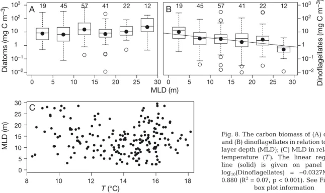
temper-atures <14°C. This has also been observed in other studies (Jahnke & Baumann 1987). According to the ‘Margalef mandala’, the stability of the water column is an important factor in controlling phyto-plankton succession (Margalef 1978). Changes in MLD had no significant influence on the diatom biomass (Fig. 8A). By contrast, dinoflagellates showed significantly higher biomass with low MLD and stronger stratification (Fig. 8B). Stratification is often linked with warming of the surface ocean; however, MLD can be regionally decoupled with temperature, which can occur at Stn L4 (p > 0.05, Fig. 8C). Thus, our analysis showed that increasing dinoflagellate biomass was firstly associated with a positive increase in temperature, and secondly, the decrease in MLD had a significant additive effect (p < 0.001).
● ●
● ●
● ●
0 5 10 15 20 25 30
19 ● 45 ● 57 ● 41 ● 22 ● 12 ●
Diatoms (mg C m
−3 )
A
● ● ● ● ● ● ● ● ●● ● ● ● ●0 5 10 15 20 25 30
10−2 10−1 1 10 102 103 10−2 10−1 1 10 102 103 19 ● 45 ● 57 ● 41 ● 22 ● 12 ●
Dinoflagellates (mg C m
−3 )
B
MLD (m) ● ● ● ● ● ● ● ● ● ● ● ● ● ● ● ● ● ● ● ● ● ● ● ●● ● ● ● ● ● ● ● ● ● ● ● ● ● ● ● ● ● ● ● ● ● ● ● ● ● ● ● ● ● ● ● ● ● ● ● ● ● ● ● ● ● ● ● ● ● ● ● ● ● ● ● ● ● ● ● ● ● ● ● ● ● ● ● ● ● ● ● ● ● ● ● ● ● ● ● ● ● ● ● ● ● ● ● ● ● ● ● ● ●● ● ● ● ● ● ● ● ● ● ● ● ● ● ● ● ● ● ● ● ● ● ● ● ● ● ● ● ● ● ● ● ● ●● ● ● ● ● ● ● ● ● ● ● ● ● ● ● ● ● ● ● ● ● ● ● ● ● ● ● ● ●● ● ● ● ● ● ● ● ● ● ● ● ● ● ● ● ● ● ●8 10 12 14 16 18
0 5 10 15 20 25 30
T (°C)
MLD (m)
C
Fig. 8. The carbon biomass of (A) diatoms and (B) dinoflagellates in relation to mixed layer depth (MLD); (C) MLD in relation to temperature (T ). The linear regression line (solid) is given on panel (B) as log10(Dinoflagellates) = −0.0327MLD +
0.880 (R2= 0.07, p < 0.001). See Fig. 2 for
Optimal growth temperatures and activation ener-gies indicate how phytoplankton respond to the changes in temperature (Chen et al. 2014). In the WEC, key diatom species were adapted to relatively lower temperatures (Fig. 7B,D), which resulted in the inverse relationship between diatom biomass and temperature (Fig. 4B). By comparison, Karenia
miki-motoioccurred at higher temperatures (Fig. 7E) and
was then succeeded by Prorocentrum cordatum. Such species succession may be indicative of a com-petitive advantage at increasing global tempera-tures, which can act as a key driver to the seasonal phytoplankton community succession. This has also been observed in other regions such as the North Atlantic (McQuatters-Gollop et al. 2007a) and the Scotian Shelf, where changes in phytoplankton com-munity structure closely follow temperature, which in turn modifies PB
m(Bouman et al. 2005). Long-term observation of variability in PB
m at
coastal sites is one of the principal factors in explain-ing the seasonal variability in primary production (Gallegos 2014). PB
mis often described as a function of temperature, typically as an Eppley curve or sev-enth-order polynomial (Eppley 1972, Cote & Platt 1983, Behrenfeld & Falkowski 1997). In the WEC, we found that a hyperbolic function between PB
m and
temperature explained a significant proportion of the variance, with increasing PB
m at lower temperature then reaching a plateau at higher temperature. By contrast, in the Scotian Shelf, an Eppley temperature dependency of PB
mgave a better fit (Bouman et al. 2005). The differences probably arise because the lowest temperature during spring in the WEC was ~7°C, and below this value, the relationship between
PB
m and temperature may assume the more typical Eppley type curve. The intercept of 8 given in Eq. (4), therefore, arises from the fact that the temperature does not go below 7°C from spring to autumn at Stn L4 and is region-specific. By contrast, in the eastern Canadian Arctic, where the temperature range is −2 to 9°C, PB
mhas been observed to follow a similar seg-mented response, with a stable upper envelope of 2.0 mg C mg−1chl ah−1at a temperature > 0°C (Li et al. 1984), suggesting different temperature depend-encies in different domains or regions. Since PB
mis a
rate normalized to chl a, the paralleled changes in carbon fixation and cellular content of pigments could result in a constant PB
mover a specific temper-ature range. Similar characteristics have been observed in diatoms such as Phaeodactylum
tricor-nutumin culture studies (Li & Morris 1982). In the
WEC, although phytoplankton species acclimate to different temperature regimes (Fig. 7, Table 1), the
relationship between PB
mand temperature could be modified by species succession. The linear increase in PB
mfrom 7 to 11°C is therefore also accompanied by a change between diatoms and nano-eukaryotes, and the plateau corresponds to an increase in dino-flagellate and coccolithophorid biomass. A similar scenario has been observed in the neighbouring cen-tral WEC, where high PB
m was accompanied with increasing pico-phytoplankton biomass (Napoléon et al. 2014). Although the upper limit of PB
m over the temperature range in the plateau is quite constant, cellular chl a:carbon ratio and growth rates may in -crease with temperature when nutrients are replete (Geider 1987). From the WEC time series data, this relationship was not evident.
Effect of nutrients on phytoplankton composition and photosynthesis in the WEC
Photosynthesis is regulated by nutrients, which, when replete, give rise to the spring bloom as day length increases from winter to spring (Platt et al. 1992). Nutrients determine the photosynthetic effi-ciency and growth rates of phytoplankton (Sosik & Mitchell 1994) since light-saturated rates of photo-synthesis are regulated by the photo-synthesis of chl a,
which is coupled to nitrate assimilation (Geider et al. 1998). Models of photosynthetic rates have therefore been developed based on nutrient status of phyto-plankton under replete or limited conditions (Geider et al. 1998, Behrenfeld et al. 2002). These studies suggest that when nutrients are depleted, photosyn-thetic rates are low, and under replete conditions,
PB
m or optimum photosynthetic rates in crease. This should also be coupled with temperature, which can co-vary with DIN, SRP and DSi over specific temper-ature ranges (Fig. 2). Previous work has shown, how-ever, that when nutrients are replete, further in creases in temperature have little effect on the phytoplank-ton biomass (Moss et al. 2003). From time series data in the WEC using nutrient concentrations alone we were unable to establish any tangible relationships with phytoplankton community structure. In the WEC from April to September, high DIN occurs under 2 different scenarios (Fig. 2A). The first is in spring, with high DIN resulting from previous winter mixing (Smyth et al. 2010). The second occurs in summer, when there can be occasional spikes in DIN as a result of high rainfall and therefore river run-off (Rees et al. 2009). The influence of these can be detected in the phytoplankton biomass as peaks in both chl aand total biomass during the spring at
tem-peratures of 9 to 10°C and during summer, when temperatures are between 14 and 16°C (Fig. 3A,B). These peaks in phytoplankton biomass do not cor -relate directly with ambient nutrient concentrations (Fig. 6), as there is evidently a lag between high nutrient concentrations and phytoplankton growth. Agawin et al. (2000) and Maranón et al. (2012) have also shown that ambient nutrient concentrations may be uncoupled from changes in phytoplankton bio-mass. Nutrients can be high when phytoplankton biomass is low (e.g. during winter when nutrients are high, but there is light limitation). By comparison, at the peak of a bloom when phytoplankton biomass is high, DIN, SRP or DSi may be used up rapidly and therefore be low. Phytoplankton biomass and nutri-ents are out of phase, resulting from the lag response between injection of nutrients into the euphotic zone and phytoplankton growth. This can be further com-plicated by the fact that the nutrient supply may often be sporadic and not constant or continuous. From nutrient concentrations alone, it is therefore difficult to formulate robust relationships between phytoplankton community structure and photo -synthesis.
The ‘irradiance-nitrate trade-off’ (Harrison et al. 1990, Irwin et al. 2012) concept suggested that (1) diatoms live in high turbulence, high nutrient envi-ronments, such as cool and well-mixed waters, and (2) dinoflagellates are favoured in low turbulence, low nutrient environments. Similar to concept (1), Paerl et al. (2006) observed abrupt changes in the phytoplankton community structure during summer hurricanes, when diatoms responded to high river runoff and a lower residence time in the water col-umn and outcompeted dinoflagellates. In the WEC, Rees et al. (2009) also showed that during episodic high river runoff in summer, the centric diatom
Chaetoceros debilis dominated and could
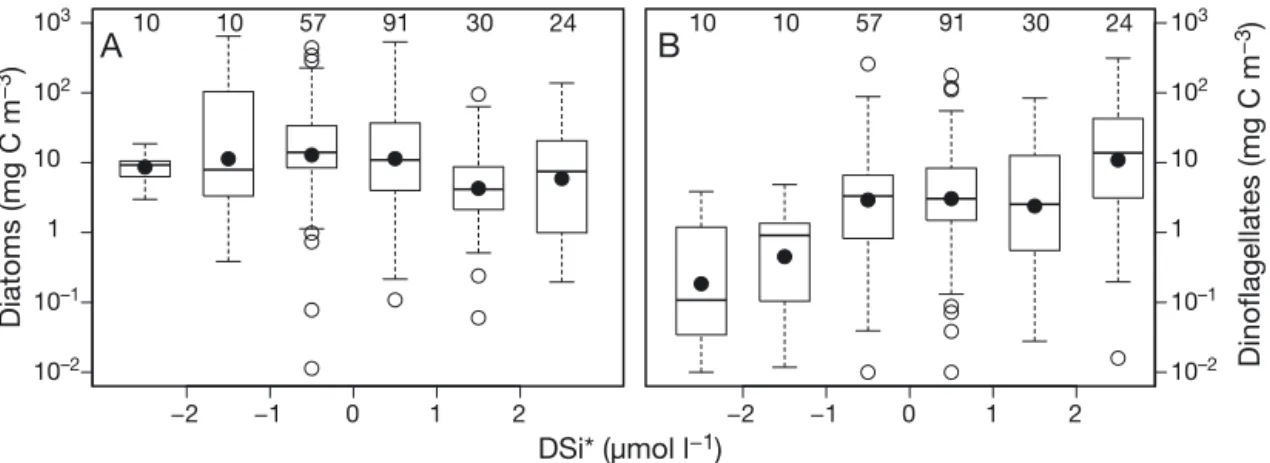
outcom-pete dinoflagellates. Other studies have shown that nano-phytoplankton often exhibit an initial response to nutrient enhancement that can occur in upwelling systems, which is then followed by diatoms (Tilstone et al. 1999). In our analysis in the WEC, diatoms did not respond to high summer temperatures even when silicate was high (Figs. 2C & 9A, Table 1), but these periods were dominated by dinoflagellates (Fig. 9B, Table 1). In contrast, laboratory studies have shown that diatoms favour high Si:N ratios (Sommer 1994). Dinoflagellate blooms in the WEC during sum-mer occurred at warsum-mer temperatures during high stratification (Figs. 4 & 8). This in turn promoted a higher photosynthetic response (Fig. 5A). Similarly in the NE Atlantic, the frequency of dinoflagellate blooms has been strongly and positively correlated with salinity (from the Atlantic inflow), temperature and wind speed (Edwards et al. 2006). The increase in dinoflagellate biomass at Stn L4 resulted in a reduction of DIN and SRP, which resulted in an excess of DSi (Fig. 9B). In contrast to observations in the NE Atlantic, we found that in the WEC during the summers of 2009 to 2012, when there was an in -crease in seasonal wind speeds, there was a parallel decrease in the biomass of dinoflagellates (Fig. 10). This may be in part due to the fact that turbulence has been shown to prevent the motile migration of dinoflagellates, which reduces their ability to com-pete for resources (White 1976, Thomas & Gibson 1990, Berdalet 1992). We also observed low biomass of dinoflagellates associated with deep MLDs (Fig. 8B), resulting from the higher wind speeds (Fig. 10). The prevalent scenario in the English Channel is that after winter mixing and the onset of stratification in spring diatom biomass increases at varying times in different locations, depending on the strength of the
● ● ●
● ● ● ●
● ● ●
●
−2 −1 0 1 2
10
● 10
● 57
● 91
● 30
● 24
●
Diatoms (mg C m
−3
)
A
● ●
● ●
● ● ●
● ●
●
−2 −1 0 1 2
10–2
10–1
1 10
102
103
10–2
10–1
1 10
102
103 10
● 10
● 57
● 91
● 30
● 24
●
Dinoflagellates (mg C m
−3
)
B
DSi* (µmol l−1)
Fig. 9. Changes in carbon biomass of (A) diatoms and (B) dinoflagellates as a function of DSi*, defined as the difference between dissolved silicate (DSi) and dissolved inorganic nitrogen (DIN). See Fig. 2 for box plot information
stratification and the attendant effects on diatoms in suspension (Ragueneau et al. 1996). Under these conditions, diatoms (e.g. Rees et al. 2009) or nano-eukaryotes would dominate. In some coastal regions, increases in temperature coupled with an increase in precipitation as a result of changes in the jet stream can lead to higher river run-off and injection of nutri-ents into coastal regions, which in turn promotes unseasonal increases in the biomass of diatoms (Jenkins et al. 2009, Francis & Vavrus 2012). From our analysis, however, it was the dinoflagellates that dominated under these conditions during summer (Fig. 7).
The temperature–size rule predicts that phyto-plankton will become smaller in an oligotrophic, warmer ocean (Finkel et al. 2010, Morán et al. 2010), which would be accompanied by a decrease of 2.5% cell volume per 1°C (Atkinson et al. 2003). If coastal or upwelling areas are included, the temperature-size rule can become reversed due to bottom-up con-trol (Agawin et al. 2000, Maranón et al. 2012). In the WEC, the correlation between high dinoflagellate biomass and increasing temperature suggests a reversal of the temperature–size relationship. This trend, however, may be forced by the ambient nutri-ent regime, as suggested in Fig. 9A. Thus, when nutrients are not limiting, this trend may modify the temperature–size rule through inter-specific compe-tition and selective grazing pressure. Different eco-logical strategies will therefore aid specific species to out-compete others under certain environmental conditions. In the light of this in the WEC, increasing temperature and nutrients during localised stratifica-tion as a result of climate change and high precipita-tion will promote the growth of dinoflagellates (Figs. 4D & 9B), which will in turn cause an increase in photosynthetic rates.
CONCLUSIONS
Analysis of ~14 yr of phytoplankton biomass and photosynthetic parameters in relation to temperature and nutrients was conducted at a coastal station in the WEC. Dinoflagellate and coccolithophorid bio-mass exhibited a positive correlation with tempera-ture, whereas diatoms had a negative correlation.
PB
m assumed a hyperbolic response to increasing temperature, reaching a plateau at 12°C. There was no correlation between nutrient levels and phyto-plankton biomass or photosynthetic rate. The major phytoplankton groups occupied specific thermal niches, which in turn modified PBm. The highest PBm occurred at higher temperatures during stratification when dinoflagellates bloomed. The analysis suggests that the dinoflagellate species such as Karenia
miki-moitoand Prorocentrum cordatummay have a
selec-tive advantage under warmer climatic conditions.
Acknowledgements. We thank the crew of RV Plymouth Quest. We thank 3 anonymous reviewers for their com-ments, which significantly improved this manuscript. Y.X. was supported by the Chinese State Scholarship Fund to study in Plymouth Marine Laboratory as a joint PhD student (Grant No. 201206310058). G.H.T. was supported by the European Union contract Information System on the Eutrophication of our Coastal Seas (ISECA) (Contract no. 07-027-FR-ISECA) funded by INTERREG IVA 2 Mers Seas Zeeën Cross-border Cooperation Programme 2007−2013. C.W., E.M.S.W. and C.H. were supported by the NERC National Capability western English Channel Observatory. M.K.B. was funded by was supported by a NERC stu-dentship (NE/F012608/1).
LITERATURE CITED
Agawin NS, Duarte CM, Agusti S (2000) Nutrient and tem-perature control of the contribution of picoplankton to phytoplankton biomass and production. Limnol Oceanogr 45: 591−600
Atkinson D, Ciotti BJ, Montagnes DJ (2003) Protists de -crease in size linearly with temperature: ca. 2.5% C−1.
Proc R Soc B 270: 2605−2611
Behrenfeld MJ, Falkowski PG (1997) Photosynthetic rates derived from satellite-based chlorophyll concentration. Limnol Oceanogr 42: 1−20
Behrenfeld MJ, Marañón E, Siegel DA, Hooker SB (2002) Photoacclimation and nutrient-based model of saturated photosynthesis for quantifying oceanic primary production. Mar Ecol Prog Ser 228:103–117
Berdalet E (1992) Effects of turbulence on the marine dino-flagellate Gymnodinium nelsonii.J Phycol 28: 267−272 Bouman H, Platt T, Sathyendranath S, Stuart V (2005)
De pendence of light-saturated photosynthesis on tem-perature and community structure. Deep Sea Res I 52: 1284–1299
Boyd PW, Strzepek R, Fu F, Hutchins DA (2010) Environ-mental control of open-ocean phytoplankton groups: now and in the future. Limnol Oceanogr 55: 1353−1376
● ●
0 3 6 9 12 15
●
● ● ●
● ●
● ●
●
●
●
● 1
10
102
103
● ●
●
● ●
● ●
● ●
W
ind speed (m s
−1
)
Dinofla
g
ellates (m
g
C m
−3
)
2004 2006 2008 2010 2012
Year
Fig. 10. Annual variability in wind speed (white bars) and dinoflagellate biomass (grey-shaded bars) from July to September, 2004–2012, at Stn L4 in the western English
Channel. See Fig. 2 for box plot information
➤
➤
➤
➤
Brewer PG, Riley JP (1965) The automatic determination of nitrate in sea water. Deep-Sea Res Oceanogr Abstr 12: 765−772
Chen B, Liu H, Huang B, Wang J (2014) Temperature effects on the growth rate of marine picoplankton. Mar Ecol Prog Ser 505: 37−47
Cote B, Platt T (1983) Day-to-day variations in the spring– summer photosynthetic parameters of coastal marine phytoplankton. Limnol Oceanogr 28: 320−344
Edwards M, Johns D, Leterme S, Svendsen E, Richardson A (2006) Regional climate change and harmful algal blooms in the northeast Atlantic. Limnol Oceanogr 51: 820–829 Eppley RW (1972) Temperature and phytoplankton growth
in the sea. Fish Bull 70: 1063−1085
Feng Y, Hare CE, Leblanc K, Rose JM and others (2009) Effects of increased pCO2and temperature on the North
Atlantic spring bloom. I. The phytoplankton community and biogeochemical response. Mar Ecol Prog Ser 388: 13−25
Finkel ZV, Beardall J, Flynn KJ, Quigg A, Rees TAV, Raven JA (2010) Phytoplankton in a changing world: cell size and elemental stoichiometry. J Plankton Res 32: 119−137 Francis JA, Vavrus SJ (2012) Evidence linking Arctic ampli-fication to extreme weather in mid-latitudes. Geophys Res Lett 39: L06801, doi: 10.1029/2012GL051000 Fu FX, Warner ME, Zhang Y, Feng Y, Hutchins DA (2007)
Effects of increased temperature and CO2 on photo
-synthesis, growth, and elemental ratios in marine Syne-chococcusand Prochlorococcus(Cyanobacteria). J Phy-col 43: 485−496
Gallegos CL (2014) Long-term variations in primary produc-tion in a eutrophic sub-estuary. I. Seasonal and spatial patterns. Mar Ecol Prog Ser 502: 53−67
Geider RJ (1987) Light and temperature dependence of the carbon to chlorophyll a ratio in microalgae and cyano-bacteria: implications for physiology and growth of phytoplankton. New Phytol 106: 1−34
Geider RJ, MacIntyre HL, Kana TM (1998) A dynamic re -gulatory model of phytoplanktonic acclimation to light, nutrients, and temperature. Limnol Oceanogr 43: 679–694 Harley CDG, Randall AH, Hultgren KM, Miner BG and oth-ers (2006) The impacts of climate change in coastal mar-ine systems. Ecol Lett 9: 228−241
Harrison PJ, Thomason PA, Calderwood GS (1990) Effects of nutrient and light limitation on the biochemical composi-tion of phytoplankton. J Appl Phycol 2: 45−56
Hawkins SJ, Southward AJ, Genner MJ (2003) Detection of environmental change in a marine ecosystem — evidence from the western English Channel. Sci Total Environ 310: 245−256
Hughes L (2000) Biological consequences of global warm-ing: is the signal already apparent? Trends Ecol Evol 15: 56−61
Hydes D, Aoyama M, Aminot A, Bakker K and others (2010) Determination of dissolved nutrients (N, P, Si) in seawa-ter with high precision and inseawa-ter-comparability using gas-segmented continuous flow analysers. In: The GO-SHIP repeat hydrography manual: a collection of expert reports and guidelines. IOCCP Rep No 14, ICPO Publ Ser No 134, v 1, 2010. UNESCO/IOC, www.go-ship.org/ Hydro Man.htm
IPCC (2007) Climate Change 2007: the physical science basis. Contribution of Working Group I to the Fourth Assessment Report of the Intergovernmental Panel on Climate Change. Cambridge University Press, Cambridge
Irwin AJ, Nelles AM, Finkel ZV (2012) Phytoplankton niches estimated from field data. Limnol Oceanogr 57: 787−797 Jahnke J, Baumann MEM (1987) Differentiation between
Phaeocystis pouchetii(Har.) Lagerheim and Phaeocystis globosaScherffel. Hydrobiol Bull 21: 141−147
Jenkins GJ, Murphy JM, Sexton DMH, Lowe JA, Jones P, Kilsby CG (2009) UK climate projections: briefing report. Met Office Hadley Centre, Exeter
Kirkwood DS (1989) Simultaneous determination of selected nutrients in seawater. Int Coun Explor Sea (ICES) CM 29 Lancelot C, Billen G, Sournia A, Weisse T and others (1987)
Phaeocystisblooms and nutrient enrichment in the conti-nental coastal zones of the North Sea. Ambio 16: 38−46 Li WKW, Morris I (1982) Temperature adaptation in
Phaeo-dactylum tricornutum Bohlin: photosynthetic rate com-pensation and capacity. J Exp Mar Biol Ecol 58: 135−150 Li WKW, Smith JC, Platt T (1984) Temperature response of photosynthetic capacity and carboxylase activity in Arc-tic marine phytoplankton. Mar Ecol Prog Ser 17: 237−243 Mantoura RFC, Woodward EMS (1983) Optimization of the indophenol blue method for the automated determina-tion of ammonia in estuarine waters. Estuar Coast Shelf Sci 17: 219−224
Maranón E, Cermeno P, Latasa M, Tadonléké RD (2012) Temperature, resources, and phytoplankton size struc-ture in the ocean. Limnol Oceanogr 57: 1266−1278 Margalef R (1978) Life-forms of phytoplankton as survival
alternatives in an unstable environment. Oceanol Acta 1: 493−509
McQuatters-Gollop A, Raitsos DE, Edwards M, Attrill MJ (2007a) Spatial patterns of diatom and dinoflagellate sea-sonal cycles in the NE Atlantic Ocean. Mar Ecol Prog Ser 339: 301−306
McQuatters-Gollop A, Raitsos DE, Edwards M, Pradhan Y, Mee LD, Lavender SJ, Attrill MJ (2007b) A long-term chlorophyll dataset reveals regime shift in North Sea phytoplankton biomass unconnected to nutrient levels. Limnol Oceanogr 52: 635−648
Menden-Deuer S, Lessard EJ (2000) Carbon to volume rela-tionships for dinoflagellates, diatoms, and other protist plankton. Limnol Oceanogr 45: 569−579
Morán XAG, López-Urrutia Á, Calvo-Díaz A, Li WKW (2010) Increasing importance of small phytoplankton in a warmer ocean. Glob Change Biol 16: 1137−1144 Moss B, McKee D, Atkinson D, Collings SE and others (2003)
How important is climate? Effects of warming, nutrient addition and fish on phytoplankton in shallow lake microcosms. J Appl Ecol 40: 782−792
Napoléon C, Fiant L, Raimbault V, Riou P, Claquin P (2014) Dynamics of phytoplankton diversity structure and pri-mary productivity in the English Channel. Mar Ecol Prog Ser 505: 49−64
Nixon SW (1995) Coastal marine eutrophication: a defini-tion, social causes, and future concerns. Ophelia 41: 199−219
Paerl HW, Valdes LM, Peierls BL, Adolf JE, Harding LWJ (2006) Anthropogenic and climatic influences on the eutrophication of large estuarine ecosystems. Limnol Oceanogr 51: 448−462
Pingree R (1980) Physical oceanography of the Celtic Sea and English Channel. In: Banner FT (ed) The north-west European shelf seas: the sea bed and the sea in motion. II. Physical and chemical oceanography and physical resources. Elsevier, Amsterdam p 415−465
Platt T, Gallegos C, Harrison W (1980) Photoinhibition of
➤
➤
➤
➤
➤
➤
➤
➤
➤
➤
➤
➤
➤
➤
➤
➤
➤
➤
➤
➤
➤
➤
➤
➤
➤
➤
photosynthesis in natural assemblages of marine phyto-plankton. J Mar Res 38: 687−701
Platt T, Sathyendranath S, Ulloa O, Harrison WG, Hoepffner N, Goes J (1992) Nutrient control of phytoplankton pho-tosynthesis in the Western North Atlantic. Nature 356: 229–231
R Development Core Team (2013) R: a language and en -vironment for statistical computing. R Foundation for Statistical Computing, Vienna, available at www.r-project. org
Rabalais NN, Turner RE, Díaz RJ, Justi D (2009) Global change and eutrophication of coastal waters. ICES J Mar Sci 66: 1528−1537
Ragueneau O, Queguiner B, Treguer P (1996) Contrast in biological responses to tidally-induced vertical mixing for two macrotidal ecosystems of Western Europe. Estuar Coast Shelf Sci 42: 645−665
Rahmstorf S, Coumou D (2011) Increase of extreme events in a warming world. Proc Natl Acad Sci USA 108: 17905−17909
Rayner NA, Parker DE, Horton EB, Folland CK and others (2003) Global analyses of sea surface temperature, sea ice, and night marine air temperature since the late nine-teenth century. J Geophys Res D 108: 4407, doi: 10/1029/ 2002JD002670
Rees AP, Hope SB, Widdicombe CE, Dixon JL, Woodward EMS, Fitzsimons MF (2009) Alkaline phosphatase activ-ity in the western English Channel: elevations induced by high summertime rainfall. Estuar Coast Shelf Sci 81: 569−574
Richardson AJ, Schoeman DS (2004) Climate impact on plankton ecosystems in the Northeast Atlantic. Science 305: 1609−1612
Riegman R, Noordeloos AAM, Cadée GC (1992) Phaeocystis
blooms and eutrophication of the continental coastal zones of the North Sea. Mar Biol 112: 479−484
Schoemann V, Becquevort S, Stefels J, Rousseau V, Lancelot C (2005) Phaeocystis blooms in the global ocean and their controlling mechanisms: a review. J Sea Res 53: 43−66
Smyth TJ, Fishwick JR, Lisa AM, Cummings DG and others (2010) A broad spatio-temporal view of the western Eng-lish Channel observatory. J Plankton Res 32: 585−601
Sommer U (1994) Are marine diatoms favoured by high Si: N ratios? Mar Ecol Prog Ser 115: 309−315
Sosik HM, Mitchell BG (1994) Effects of temperature on growth, light absorption, and quantum yield in Duna -liella tertiolecta(Chlorophyceae). J Phycol 30: 833–840 Southward AJ, Langmead O, Hardman-Mountford NJ,
Aiken J and others (2004) Long-term oceanographic and ecological research in the western English Channel. Adv Mar Biol 47: 1−105
Suzuki Y, Takahashi M (1995) Growth responses of several diatom species isolated from various environments to temperature. J Phycol 31: 880−888
Thomas WH, Gibson CH (1990) Quantified small-scale tur-bulence inhibits a red tide dinoflagellate, Gonyaulax polyedraStein. Deep-Sea Res A 37: 1583−1593
Thomas MK, Kremer CT, Klausmeier CA, Litchman E (2012) A global pattern of thermal adaptation in marine phyto-plankton. Science 338: 1085−1088
Tilstone GH, Figueiras F, Fermín E, Arbones B (1999) Signif-icance of nanophytoplankton photosynthesis and pri-mary production in a coastal upwelling system (Ría de Vigo, NW Spain). Mar Ecol Prog Ser 183: 13−27
Tilstone GH, Figueiras F, Lorenzo LM, Arbones B (2003) Phytoplankton composition, photosynthesis and primary production during different hydrographic conditions at the Northwest Iberian upwelling system. Mar Ecol Prog Ser 252: 89−104
Uncles R, Stephens J (1990) The structure of vertical current profiles in a macrotidal, partly-mixed estuary. Estuaries 13: 349−361
Welschmeyer NA (1994) Fluorometric analysis of chloro-phyll ain the presence of chlorophyll band pheopig-ments. Limnol Oceanogr 39: 1985−1992
White AW (1976) Growth inhibition caused by turbulence in the toxic marine dinoflagellate Gonyaulax excavata.
J Fish Res Board Can 33: 2598−2602
Widdicombe CE, Eloire D, Harbour D, Harris RP, Somerfield PJ (2010) Long-term phytoplankton community dynam-ics in the western English Channel. J Plankton Res 32: 643−655
Zhang JZ, Chi J (2002) Automated analysis of nanomolar concentrations of phosphate in natural waters with liquid waveguide. Environ Sci Technol 36: 1048−1053
Editorial responsibility: Graham Savidge, Portaferry, UK
Submitted: February 7, 2014; Accepted: October 25, 2014 Proofs received from author(s): December 20, 2014