Sharif University of Technology
Scientia IranicaTransactions B: Mechanical Engineering www.scientiairanica.com
Matched pole-zero state-space model and
continuous-time properties
A.H.D. Markazi
School of Mechanical Engineering, Iran University of Science and Technology, Narmak, Tehran, P.O. Box 16844, Iran. Received 8 May 2011; received in revised form 11 August 2012; accepted 28 January 2013
KEYWORDS Matched pole/zero; Plant-Input Mapping (PIM) method; Discretization; Digital redesign; Sampled-data.
Abstract. The Matched Pole-Zero (MPZ) model is a widely used technique for discrete-time approximation of continuous-discrete-time controllers. In this article, a new state-space representation for the (MPZ) model is presented. The new formulation can be used for direct discretization of state-space controllers, and can be easily automated on a digital computer. The most important advantage of the proposed representation is that it preserves the dynamic structure of the original continuous-time realization, i.e. the physical meaning of the states and the direction of eigenvectors remain unchanged. In fact, the new method provides, exactly, the same dynamic state equations as the step-invariant model, together with some modications on the static output state equation.
Up to now, due to the lack of such eigenstructure-preserving state-space representa-tions, most of the time domain studies on the eects of discrete approximation of analog controllers were mostly performed using the step-invariant model, although that method is seldom used for actual discretization of controllers. The new formulation paves the way for extending those studies to the case of the more widely used MPZ method.
c
2013 Sharif University of Technology. All rights reserved.
1. Introduction
Despite the existence of numerous methods and lit-erature on the direct design of sampled-data control systems ([1-7] etc.), there remain motivations to use the more conventional digital redesign methods (indirect methods) in which a predesigned analog controller is approximated by a digital one. These motivations include better physical insight and availability of a wide spectrum of continuous control design meth-ods. There exists a number of well known methods for discretization of nite-dimensional continuous-time controllers/plants [8-10]. Other methods also exist for discretization of innite-dimensional controllers [11], nonlinear systems [12] and multi-rate controllers [13]. One group of such methods, including the method of
*. Corresponding author. Tel: +98-21-77491241; Fax: +98-21-77240488
E-mail address: [email protected] (A.H.D. Markazi)
Tustin, are based upon numerical approximation of the integration operator, which can be used for dis-cretization of controllers. The other group, including the step-invariant model, provides an exact discrete model for a plant with a given hold element. The Matched Pole/Zero (MPZ) discretization technique is yet another method which is not directly motivated by the numerical approximation of integrators or the concept of hold equivalence. In this method, the zeros and poles of the continuous system are mapped by the relation, esh, where s is a pole or zero, and h is
the sampling period. The MPZ technique has been extensively used and proved to be ecient for discrete approximation of continuous-time controllers [8]. This method also plays a central role in a new closed-loop digital redesign method, called the Plant-Input Mapping (PIM) method ([14,15], which guarantees closed-loop stability for all nonpathological sampling periods.
Tustin's and zoh-equivalent models, no state-space algorithms were introduced for the MPZ method until recently. This fact seems to be the main reason for most research to ignore usage of the MPZ method for analytical studies of sampled-data systems.
A number of attempts and studies have been re-ported on state-space algorithms for the MPZ method. An interesting interpretation of the MPZ model, based on the generalized hold equivalence concept, was pro-posed in [16,17]. This method, however, involved tedious hand calculations, which could not be easily performed, even for low order systems. A simpler state-space algorithm was introduced in [18]. That method had two drawbacks:
1. It was only applicable to systems with a realization in the observable canonical form;
2. It involved inversion of some controllability matri-ces which are known to be ill-conditioned for higher order systems ([19], page 105).
Among common discretization methods, the only one used to preserve the structure of original continu-ous realization was the step-invariant method. In other words, the step-invariant model exceptionally preserves the physical meanings of the states and the direction of system eigenvectors. That is why most time-domain studies on the properties of discretized sampled-data systems are based on controllers which are discretized using the step-invariant method (e.g., see [2,3]). This is despite the fact that the step-invariant method is seldom used for discretization of controllers in practice. The main objective of this paper is to provide a state-space realization, with similar advantages, for the MPZ model. The new formulation should pave the way for further time-domain studies with the more widely used MPZ method, which, compared to the step-invariant method, is much better suited for discretization of controllers.
2. MPZ technique
2.1. Transfer function version
Consider a strictly stable SISO transfer function: g(s) =
Qm
i=1(s i)
Qn
i=1(s i); m n: (1)
The MPZ discrete-time approximation technique is partly motivated by the z-transform method in which the poles of g(s) are mapped to the z-plane, according to the relation z = ehs, where h is the sampling period.
In fact, the MPZ technique extends such a mapping to the case of zeros as well as poles. In particular, the discrete system, gd(z), is obtained by the following
procedure [9]:
1. All of the poles and nite zeros of g(s) are mapped with the relation z = ehs;
2. All but one of the innite zeros, if any, are mapped to the points f 1g (The relative degree of 1 ensures the physical realizability of gd(z));
3. The dc-gain of the two transfer functions are matched, such that:
lim
s!0g(s) = limz!1gd(z):
2.2. Proposed state-space version
Consider a stable SISO continuous-time system with a minimal state-space realization, G := fA; b; c; dg, where A 2 Rnn, b 2 Rn1, c 2 R1n, and d is a
scalar. The objective is to nd a state-space realization, Gd := fAd; bd; cd; ddg such that the (transmission)
zeros and the eigenvalues of G are mapped according to the procedure described in Section 2.1.
The proposed state-space algorithm for the above problem is introduced below.
3. Proposed state-space algorithm 3.1. Bi-proper system
For the time being, assume that, g(s) is bi-proper, i.e. m = n. Let us dene the matrix Ad as Ad =
eAh. This assures that the eigenvalues (poles) of the
discrete system, i.e. f1; 2; ; ng, are mapped by
the relation eih, as desired.
Provision of a state-space formulation for similar mapping of the zeros is more subtle and needs some elaboration. Following the well-known MATLAB syn-tax, let us dene the tzero operator as the operator acting on system G and providing the nite (transmis-sion) zeros of G, i.e.:
= [1; 2; ; n] = tzero(G); (2)
where is the vector of nite zeros of G. Robust algorithms exist for computing the zeros of LTI systems ([20], for example). By denition of the MPZ model, the nite zeros of Gdare required to be at the locations
given by the vector:
d:= [exp(h)]; (3)
where exp(h) is the element-wise exponential of vector h.
It can be shown that the following expression relates the state-space realization of Gd to its transfer
function, gd(z); (see [21], page 651):
gd(z) = det(zI e Ah+b
dcd)+(dd 1)det(zI eAh)
det(zI eAh) :
(4) Now, by arbitrarily xing dd as dd = 1, the
nding bd and cd, such that the eigenvalues of matrix
[eAh bdcd] are placed at the locations given by the
elements of vector d. Let us also x bd, as bd =
b. Now, the problem reduces to nding cd, such
that the eigenvalues of [eAh bdcd] are placed at d.
This is a standard eigenvalue placement problem for which robust algorithms exist [19,22]. Existence of the solution for cd is guaranteed by controllability of the
pair feAh; bg, which is obvious due to the controllability
of the pair fA; bg and the fact that A and eAh share
the same set of eigenvectors ([21], page 661).
Finally, in order to match the steady-state gains of the two systems, the nal vector, cd, and also ddare
obtained by multiplying the previous cd and dd by a
gain correction factor, kd, given by:
kd= c( A) 1b + d
cd(In Ad) 1bd3+ dd: (5)
Remark 1. Instead of selecting bd, and then
cal-culating cd, one may x cd, and then calculate bd
accordingly. This, in fact, provides an extra exibility to the method which can prove useful in practice, as it allows the designer to preserve the structure of the discrete system, from the point of view of actuators or sensors, respectively. In either case, the transfer function of the discrete system remains the same. 3.2. Strictly proper system
When the relative degree of the continuous system is not zero (i.e., when m < n), the eigenvalue assignment of [eAh b
dcd] at the locations of dis not meaningfule,
because dim(d) < n: In order to resolve this problem,
Eq. (3) is replaced by: d:= [ 1=; 1; ; 1| {z }
n m 1
; exp(h)]; (6)
where is an arbitrarily selected, very small, positive number. The implication is that with dd = 1 and
Eq. (4): gd(z)=(z+
1
)(z+1) (z+1)(z eh1) (z ehm)
det(zI eAh) :
(7) Also, from Eq. (5):
kd=gg(s)js=0
d(z)jz=1; (8)
=((1) (m)
1) (n)
(1 eh1) (1 ehn) (1+1
)(1+1) (1+1)(1 eh1) (1 ehm)
1: (9)
This implies that for the scaled discrete system, kdgd(z), it turns out that dd! kddd= kd 1 h 0; for
small enough ; and also cd! kdcd:
The proposed algorithm is summarized as below: Algorithm 1. (shift form)
1. Set Ad:= eAh.
2. Set bd:= b.
3. If n = m, set dd:= 1, otherwise set dd = 0.
4. Find the vector as in Eq. (2).
5. If n = m, set the vector d as in Eq. (3), otherwise
as in Eq. (6).
6. Find cd such that the eigenvalues of Ad bdcd are
assigned at d.
7. Set cd:= kdcd, and dd:= kdddwhere kdis given by
Eq. (5).
In order to make the discrete representation of the model more similar to its continuous counterpart, and for better numerical properties when h is too small, one may prefer to use the operator, where = q 1h , and q is the common shift operator. Clearly, the -operator is intuitively closer to a continuous-time derivative than the common q operator [23,24]. That is, we may want to consider the discrete state-space system in the following form:
x[kh] = Ax[kh] + bu[kh];
y[kh] = cx[kh] + du[kh]: (10)
The state-space algorithm for this case can be formu-lated as below:
Algorithm 2. ( form)
1. Set A := (eAh I)=h.
2. Set b := b.
3. If n = m, set d := 1, otherwise set d = 0 (by
Remark 1).
4. Find the vector as in Eq. (2).
5. If n = m, set the vector := [exp(h I)=h],
otherwise, set:
:= [ 1=; 1=h; ; 1=h| {z } n m
; exp(h I)=h]:
6. Find c such that the eigenvalues of A bc are
assigned at .
7. For a very low arbitrary frequencey, , nd k from
the following: k= c(I A)
1b + d
8. Set c := kc, and d:= kd.
The following lemma characterizes a connection between the continuous and discrete realizations for small sampling periods.
Lemma 1. The discrete realization obtained by the MPZ algorithm (in form) converges to its original counterpart, when the sampling period is decreased, i.e.:
1. limh!0 A! A;
2. limh!0 c ! c;
3. limh!0 d ! d.
Proof
1. Obvious, because A = (eAh I)=h;
2. By noting that b = b, and due to the uniqueness of
the solution to the eigenvalue assignment problem in Item 6 of Algorithm 2, based on which, c is
obtained;
3. Due to Items 1 and 2 above, and Eq. (11), which implies that limh!0k ! d and, hence, d! d.
4. Time domain properties
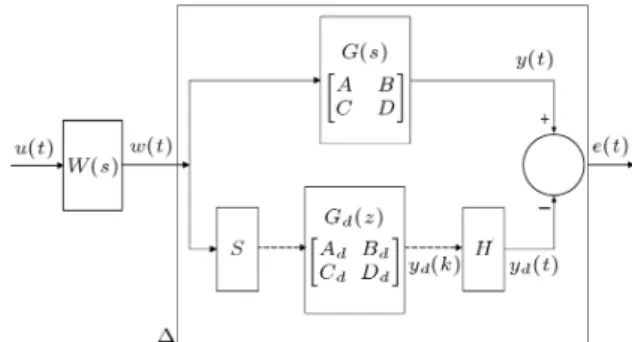
Consider the general sampled-data set up shown in Figure 1, with G being a LTI asymptotically stable system, and G the MPZ discrete-time model of G.
Here, S and H are synchronized ideal sampling and zero-order hold operators, respectively, and W is a nite-dimensional, linear and time-invariant, stable and strictly causal prelter. As shown in the gure, is the discretization error operator. In the sequel, k:k1
denotes the L1 norm of a signal and k:k
L1 denotes
the L1 induced norm of an operator acting on L1
signals.
Inclusion of W in this setup provides a sucient condition for k(I HS)W kLp to be nite for every
1 p 1; and, furthermore, (I HS)W converges to zero as h tends to zero in the sense of these norms (by Theorem 9.3.3 in [1]).
Figure 1. Discretization error in a sampled-data setting.
In this study, we will mostly utilize the lifting tech-nique for comparing the time response of a continuous-time system with its discretized counterpart. In a broad sense, the lifting technique is a method for rearranging a continuous-time periodic system, in such a way that its periodicity can be viewed as discrete-time shift invariance [4].
We will limit our discussion to the case of bounded continuous-time signal space, L1[0; 1).
We also dene `L1[0;h] to be the space of all
sequences that take their values in the Banach space L1[0; h]. Next, we dene `1
L1[0;h] as the subspace of
bounded sequences in `L1[0;h].
We will use the notation Lh : L1[0; 1) !
`L1[0;h]to denote the norm preserving lifting operator.
Suppose G is a stable linear continuous-time operator: L1[0; 1) ! L1[0; 1). The lifted version of G, noted
as G, is the linear discrete-time system acting on lL1[0;h], i.e., G : lL1[0;h]! lL1[0;h].
Considering the norm preserving property of the lifting operator, we will convert the setup of Figure 1 into an equivalent setup, as shown in Figure 2.
For the linear continuous-time system, G: fA; B; C; Dg, it can be shown [1] that the lifted system is given by G: fA; B; C; Dg, where:
A : Ax = eAhx;
B : Buk= Z h
0 e
A(h )Bu k()d;
C : (Cx)(t) = CeAtx;
D : (Duk)(t) = Duk(t) + Z t
0 Ce
A(t )Bu k()d:
(12) The kth component of the lifted output of the lifted system is given by [1]:
^y[kh + t] =
k 1
X
l=0
h
CAk 1 lBw[kh + t]i
+ Dw[kh + t];
Figure 2. Equivalent discretization problem in a lifted setting.
where:
0 t < h: (13)
Now, consider the discretized MPZ model, Gd. In order
to make the discrete-time behavior of the MPZ model comparable with its continuous counterpart, we prefer to use the operator. Using the results specied in Algorithm 2, the discrete-time output of Gd, for a given
input w[kh], can be written as: yd[kh] =
k 1
X
l=0
c(hA+I)k 1 l(hb)w(lh)
+ dw(kh): (14)
If yd[kh] is passed through a zero order hold element,
the output would be a staircase (semi) continuous signal, which, in lifted form, can be represented as:
y[kh + t] =
k 1
X
l=0
(c)(hA+ I)k 1 lh(b)w[lh]
+ (d)w[kh]; (0 t < h): (15)
Consider the setup of Figure 1, and a bounded contin-uous input, u(t) 2 L1. Dene w[kh + ] as the kth
component of the discrete vector obtained by lifting of w(t). Also, dene w[kh + ] as the deviation of w[kh + ] from its staircase equivalent, i.e.:
w[kh + ] = w[kh] + w[kh + ];
0 < h: (16)
Clearly: lim
h!0w[kh + ] = 0: (17)
Lemma 2. Let us dene the kth component of the lifted error signal as:
e[kh + t] , ^y[kh + t] y[kh + t];
0 t < h: (18)
Under the above assumptions, the following property holds:
lim
h!0
ke[kh + t]k1
kw[kh + t]k1 = 0: (19)
Proof (This proof closely follows the method of [25],
which is partially motivated by [26].) Since the lifting operator, Lh, is norm preserving, we will work with
the equivalent discretization problem in a lifted setting (Figure 2). Using Eqs. (13) and (15), the lifted outputs of G and HGdS can be, respectively, written as:
^y[kh+t]=k 1X
l=0
ceAt(eAh)k 1 l h
Z
0
eA(h s)bw[lh+s]ds
+
t
Z
0
ceA(t s)bw[kh + s]ds + dw[kh + t];
(0 t < h); y[kh+t]=k 1X
l=0
(c+c)(h(A+A)+I)k 1 lh(b)w[lh]
+ (d + d)w[kh]; (0 t < h);
where fA; c; dg ! 0, when h ! 0, by Lemma 1. With repeated use of the triangle inequality, and also, addition/subtraction of terms to allow suitable factorizations, it is tedious yet straightforward to show that the L1norm of the error is:
k^y[kh + t] y[kh + t]k1
kw[kh + t]k1 = maxt2[0;h)
(Z t 0 ce
Asbds
+ jdjkw[kh + t]k1
kw[kh + t]k1 + jdj
+
+1
X
l=0
"
c(eAh)lh(b) c(h(A + A) + I)lh(b)
+c(h(A + A) + I)lh(b)
+ Z h
0 c(e
At I)(eAh)leAsbds
+c(eAh)l Z h 0 e
Asbds h(b)!
+
Z h
0 c(e
Ah)leAsbdskw[kh + t]k1
kw[kh + t]k1 #)
:
(20) Now, we need to prove that every term in the above equation converges to zero, when h ! 0. Since G is asymptotically stable, all the eigenvalues of A are in the open left half of the s plane, hence,R0heAsds < h
eAh belong to the open unit circle in the z plane and,
hence, h+1P
l=0ke
Ahlk is nite. Therefore:
max t2[0;h) 8 < : t Z 0
ceAsbds
9 = ;kck 0 @ h Z 0
eAsds
1
Akbkh!0! 0:
As mentioned before, W provides a sucient condition for k(I HS)W kLp to be nite for every 1 p
1, and, furthermore, (I HS)W converges to zero as h tends to zero in the sense of these norms. The implication is that:
sup
kw[kh+t]k16=0
kw[kh + t]k1 kw[kh + t]j1
= sup
kw[kh+t]k16=0
k(I HS)w[kh + t]k1 kw[kh + t]k1
= sup
kW uk16=0
k(I HS)W uk1 kW uk1 h!0! 0: Therefore:
max
t2[0;h)
jdjkw[kh+t]k1
kw[kh + t]k1
=jdjkw[kh+t]k1
kw[kh + t]k1
h!0! 0:
Also: max
t2[0;h)fjdjg = jdj h!0! 0;
and: max t2[0;h) (+1 X l=0 Z h 0 jc(e
At I)(eAh)leAsbjds
)
kckeAt I +1X l=0
eAhl
!
h kbkh!0! 0;
max
t2[0;h)
(+1 X
l=0
jc(eAh)l Z h 0 e
Asbds h(b)
! j ) kck +1 X l=0 eAhl !
khb h(b)kh!0! 0;
max
t2[0;h)
( +1 X
l=0
Z h
0 jc(e
Ah)leAsbjds
! kwk1 kwk1 ) kck +1 X l=0 eAhl !
hkbkkwk1
kwk1
h!0! 0;
max
t2[0;h)
(+1 X
l=0
jc(eAh)lh(b) c(h(A + A) + I)lh(b)j
)
kck
+1
X
l=0
eAhl (h(A + A) + I)l
! hkbk
h!0! 0;
max
t2[0;h)
(+1 X
l=0
jc(h(A + A) + I)lh(b)j
) kck +1 X l=0 (h(A+A)+I)l !
hkbkh!0! 0:
Now, since for all t 2 [0; h), all the individual terms in Eq. (20) approach zero when h ! 0, the desired result is proven.
Taking the stability of G and Gd, the continuous
error signal, e(t) 2 L1[0; 1), and its lifted version,
e 2 `L1[0;h], is dened as a sequence with values in
L1[0; h], denoted byfekg, where for each k, we have:
e(k) , e[kh + t]; 0 t < h: (21) Furthermore:
kfekgk1, sup
k kekk1; fekg 2 `L1[0;h]: (22)
Considering the norm preserving property of the lifting operator, it can be deduced that:
lim
h!0ke(t)k1! 0: (23)
Now, since u(t) 2 L1 is arbitrary, then the following
holds: lim
h!0kW kL1, limh!0kuksup16=0
kek1
kuk1:u(t)2L 1!0:
(24) This property is of practical importance when an ana-log system is implemented digitally, because it assures that a better performance can be attained by using a smaller sampling period. It is interesting to note that not all of the modern digital redesign methods provide such a practically important property; for instance, see the method in [27] and examples thereof.
Example 1. With h = 0:01 sec, nd the MPZ discrete-time model of the continuous-time system:
A = 2
4 83 0:50 0:1250
0 2 0
3
5 ; b =
2 411
0 3
5 ; (25)
c =0 0:1818 0:909; d = 0: (26)
Step 1:
A = (eAh I)=h
= 2
4 7:88072:9751 0:49380:0198 0:12310:005
0:0792 1:9999 0
3 5 :
(27)
Step 2: Set b = b;
Step 3: Set d = 0, because of the nonzero relative
degree of the system;
Step 4: = [ 11; 1];
Step 5: = [ 1000; 10:9397; 0:9995];
Step 6: c = [11:9349; 997:0048; 497:7565];
Step 7: k= 1:8267e 004;
Step 8: Set new c := kc = [0:0022; 0:1821; 0:0909].
Resemblance between the discrete state-space re-alization fA; b; c; dg and the original continuous
counterpart fA; b; c; dg is obvious from the above which shows the advantage of the proposed algorithm com-pared with the transfer function approach.
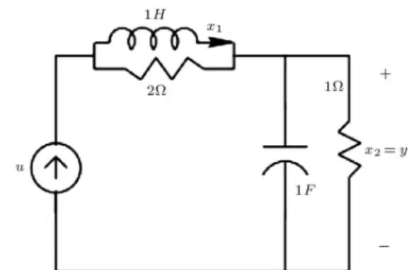
Example 2. Consider the RLC network shown in Figure 3. It can be shown that the following realization describes the dynamical behavior of this system:
_x1
_x2
=
3 1
0 1 xx12
+
2 1
u y =0 1 xx1
2
:
It can be easily seen that this system is unobservable, therefore, the algorithm proposed in [18] is not applica-ble. The MPZ model of this system using Algorithm 1
Figure 3. An unobservable RLC network.
can be obtained for h = 0:1 sec, as below:
x1(k + 1)
x2(k + 1)
=
0:7408 0:0820 0 0:9048
x1(k)
x2(k)
+
20:2
0:1
u(k); y =0 1 xx1(k)
2(k)
:
It should be noted that, unlike the form, the realization in the shift form lacks the proprty of resemblance between the discrete and continuous state-space matrices. Another point is that, in this example, use was made of Remark 1 to preserve cdinstead of bd,
so that the sensor connection of the realization could be preserved.
Example 3. Consider the following continuous sys-tem:
g(s) = 1
s2+ s + 1:
In order to study the eect of the sampling period on the continuous-time performance of the discretized system, a range of sampling period h = f0:1; 0:2; 1g is considered. The input signal is considered as a unit step function, u(t) = 1(t), which has the property u(t) 2 L1[0; 1). In order to guarantee uniform
convergence a strictly causal prelter is selected: W (s) = 1
0:5s + 1:
Table 1 shows the values of continuous-time error signal ke(t)k1over the range of pre-specied sampling
periods. Uniform convergence of the error norm can be observed in the table.
5. Concluding remarks
A new state-space algorithm is introduced for the matched pole/zero discretization technique. Unlike previously existing methods, the new algorithm is not limited to any specic realization form and can be automated by existing software packages. The robustness properties of the algorithm have been im-proved considerably, compared with the algorithm in [18], and does not include the inversion of ill-conditioned matrices that are usually encountered with high order systems and with very small sampling periods.
It is also shown in this paper that the continuous-time response of the discretized system converges to Table 1. Norm of the error signal versus sampling perio. Uniform convergence is shown here.
h 0.1 0.2 0.3 0.4 0.5 0.6 0.7 0.8 0.9 1
that of the original continuous system in the L1
-induced norm sense. This means that the maximum dierence in the time responses of the continuous and discretized systems, subject to any low-pass ltered and bounded continuous-time signal, approaches zero, when the sampling period is decreased. This property is of considerable practical importance, because it assures the designer that by reducing the sampling period, the resulting discretization error is reduced as well. It can be shown that most of the classical discretization techniques enjoy such a useful property, while there are some advanced (global) discretiza-tion methods which lack such a property. In other words, while, for a xed h, the performance of most global methods could be better than that of the local discretization methods, they may not provide the practically important assurance of improvement in performance when the sampling period is reduced. The method is limited to the SISO case. Extension to the MIMO case is not obvious and is left for future work.
References
1. Chen, T., Optimal Sampled-Data Control Systems, London, Springer-Verlag (1995).
2. Chen, T. and Francis, B.A. \H2-optimal sampled data control", IEEE Trans. Aut. Control, 36, pp. 387-397 (1991).
3. Chen, T. and Francis, B.A. \Input-output stability of sampled-data systems", IEEE Trans. Aut. Control, 36, pp. 50-58 (1991).
4. Bamieh, B.A. and Boyd Pearson, J. \A general frame-work for linear periodic systems with application to H1sampled-data control", IEEE Trans. Auto. Cont., AC-37, pp. 418-435 (1992).
5. Bamieh, B., Dahleh, A. and Boyd Pearson, J. \Mini-mization of the L1 norm for sampled-data systems", IEEE Trans. Auto. Cont., AC-38, pp. 717-732 (1993).
6. Sivashankar, N. and Khargonekar, P. \Induced norms for sampled-datasystems", Automatica, 28, pp. 1267-1272 (1992).
7. Yamamoto, Y. \A function space approach to sampled data control systemsand tracking problems", IEEE Trans. Aut. Cont., 39, pp. 703-713 (1994).
8. Ogatta, K., Discrete-Time Control Systems, Engle-wood Clis, N.J.: Prentice-Hall (1987).
9. Franklin, G.F., Powell, J.D. and Workman, M.L., Digital Control of Dynamic Systems, Addison-Wesley (1990).
10. Kowalczuk, Z. \Discrete approximations of continuous-time systems: A survey", IEE Proceedings, Control Theory and Applications, 140, pp. 264-278 (1993).
11. Kosugi, N. and Suyama, K. \Digital redesign of innite-dimensional controllers based on numerical
integration", Applied Mathematical Sciences, 6, pp. 3801-3819 (2012).
12. Nguyen-Van, T. and Hori, N. \A new class of discrete-time models for nonlinear systems through discretiza-tion of an integradiscretiza-tion gain", IET Control Theory and Applications (2013) (Accepted for publication).
13. Sakamoto, T. and Hori, N. \Multi-rate exact dis-cretization via diagonalization of a linear system: Distinct real eigenvalue case", ACTA Control and Intelligent Systems, 40, pp. 234-241, 2012.
14. Markazi, A.H.D. and Hori, N. \A new method with guaranteed stability for discretization of continuous-time control systems", in Proc. American Control Conf., 2 (Chicago, IL), pp. 1397-1402 (1992).
15. Markazi, A.H.D. and Hori, N. \Discretization of continuous-time control systems with guaranteed sta-bility", IEE Proceedings, Control Theory and Applica-tions, 142(4), pp. 323-328 (July 1995).
16. Rabbath, C. \A characterization and performance evaluation of digitally redesigned control systems", PhD thesis, McGill Univ., Montreal, Canada (1999).
17. Rabbath, C. \A structured interpretation of matched pole/zero discretization", IEE Proceedings, Control Theory and Applications, 149, pp. 257-262 (2002).
18. Davaie-Markazi, A.H. \A new algorithm for matched pole/zero discretization", in 9th IEEE International Conference on Methods and Models in Automation and Robotics (Miedzyzdroje, Poland), pp. 387-391 (August 2003).
19. Jamshidi, M., Tarokh, M. and Shafai, B., Computer-Aided Analysis and Design of Control Systems, Pren-tice Hall (1992).
20. Emami-Naeini, A. and Van Dooren, P. \Computation of zeros of linear multivariable systems", Automatica, 18, pp. 415-430 (1982).
21. Kailath, T., Linear Systems, Englewood Clis, N.J., Prentice-Hall (1980).
22. Kautsky, J., Nichols, N. and Van Dooren, P. \Robust pole assignment inlinear state feedback", Intl. J. Con-trol, 41, pp. 1129-1155 (1985).
23. Goodwin, G.C., Lozano-Leal, R., Mayne, D.Q. and Middleton, R.H. \Rapproachment between continuous and discrete model reference adaptive control", Auto-matica, 22-2, pp. 199-207 (1986).
24. Middleton, R.H. and Goodwin, G.C., Digital Con-trol and Estimation, A Unied Approach, Englewood Clis, N.J., Prentice-Hall (1990).
25. Markazi, A.H.D. and Fardad, M. \A new L1-induced norm evaluation of classical techniques for discrete-time approximation of continuousdiscrete-time functions", In-ternational Journal of Engineering Science, 12(2), pp. 135-149 (2001).
26. Rabbath, C. and Hori, N. \Continuous-time lifting analysis of digitally redesigned control systems", in Society of Intstrument and Control Engineers (SICE) Conf. (Chiba, Japan), pp. 779-774 (1998).
27. Anderson, B. and Keller, J. Control and Dynamic Sys-tems, vol. 66,ch. Discretisation Techniques in Control Systems, pp. 47-112, AcademicPress (1994).
Biography
Amir Hossein Davaie Markazi received BS, MS, and PhD degrees, respectively, from Iran University of Science and Technology, Tehran, Iran (1982), Sharif University of Technology, Tehran, Iran (1987) and
McGill University, USA (1995). He is currently Associate Professor in the school of Mechanical En-gineering at Iran University of Science and Tech-nology. Dr. Markazi is former chairman of the Iranian Society for Mechatronics, and has conducted research in the elds of digital and hybrid control of dynamic systems, adaptive, fuzzy, sliding mode control of nonlinear systems, networked control and real-time implementation of hardware-in-the-loop sys-tems.