Zhao_unc_0153D_11510.pdf

(1)

Fluid-Structure Interaction in Viscous Dominated

Flows

by Longhua Zhao

A dissertation submitted to the faculty of the University of North Carolina at Chapel Hill in partial fulfillment of the requirements for the degree of Doctor of Philosophy in the Department of Computer Science.

Chapel Hill 2010

Approved by:

Roberto Camassa, Advisor Richard M. McLaughlin, Advisor M. Gregory Forest, Committee Member

Laura Miller, Committee Member Richard Superfine, Committee Member

(2)

c

2010 Longhua Zhao

(3)

ABSTRACT

LONGHUA ZHAO: Fluid-Structure Interaction in Viscous Dominated Flows.

(Under the direction of Roberto Camassa and Richard M. McLaughlin.)

Theoretical, numerical and experimental studies for several flows in the Low Reynolds number regime are reported in this thesis. It includes the flow structure and blocking phenomena in linear shear or rotation flow past an embedded rigid body, and flows induced by a slender rod precessing a cone to imitate the motion of nodal cilia are studied with the singularity method.

(4)

emergence of a three-dimensional bounded eddy. Additionally, we study the case of a sphere embedded at a generic position in a rotating background flow, with its own prescribed rotation including fixed and freely rotating. Exact closed form solutions for fluid particle trajectories, stagnation points on the sphere, and critical points in the interior of the flow are derived.

We extend our results further to spheroids as well, where similar blocking results are documented. The broken symmetry offered by a tilted spheroid geometry induces new three-dimensional effects on the streamline deflection, which can be viewed as effective positive or negative suction in the horizontal direction orthogonal to the background flow depending on the tilt orientation. We close this study with results of a spheroid embedded in a rotating background flow, with its own prescribed tilt orientation. Net fluid transport is observed in this flow, where the direction of transport depends on the direction of the background rotation and the tilt orientation of the spheroid.

(5)

ACKNOWLEDGMENTS

In this acknowledgements, I would like to thank those persons who help me to make this thesis possible.

I would like to express my deep gratitude to my advisor Dr. Roberto Camassa who introduced me into the world of fluid mechanics and helped me with his deep insight to the problems. I also want to offer sincere appreciation to my co-advisor Dr. Richard M. McLaughlin for his in-depth guidance and great inspiration during the development of this work. Without their kind help, encouragement and support, this dissertation would not have being possible. Their helpful advice and careful guidance are invaluable for me beyond this dissertation work.

Faculty members at the Carolina Institute of the Interdisciplinary Applied Mathe-matics (CIIAM) at UNC are very helpful and friendly to me, and I want to express my appreciation to them. My special thanks go to Dr. M. Gregory Forest whose instructive and stimulating suggestions are always of great help to me, and it is a great pleasure to learn from him. I would also acknowledge my gratitude to Dr. David Adalsteisson for his patience and assistance with many technological challenges during my study and his DataTank software. I thank Dr. Jingfang Huang, who is always kind and helpful in answering my questions and giving me useful suggestions. I want to thank Dr. Laura Miller for agreeing to be on my dissertation committee and her support for my job hunting. I also want to thank Dr. Peter Mucha for the nice discussions about optimization and swimmer.

(6)

and his effort to track RMX videos. I thank David Holz, whom we met at the right time and brought us the ideal tools, for his program to track the pin in the experiments and all the discussions we have had.

This thesis has been greatly improved with helpful comments and suggestions from my advisors and other committee members. I sincerely appreciate their time and efforts. I also would like to thank the staff in the Mathematics Department, specially Brenda Bethea for her assistance throughout my graduate years.

My friends at the Department of Mathematics have always offered a friendly atmo-sphere and I am really happy for those years of study. A special acknowledgement goes to all my officemates at UNC. I wish them the best in their future.

(7)

List of Figures

2.1 Flow past a fixed sphere x2+y2 +z2 =a2. . . 11

2.2 Streamlines in the y= 0 plane. . . 18

2.3 Separation surfaces generated by separatrix lines in the flow. . . 20

2.4 Streamlines on separation surfaces close to the sphere. . . 21

2.5 “Footprint” of stagnation surfaces on the sphere. . . 24

2.6 Eigenvectors of matrix A atx= 0, y0 = 5, z = 0. . . 25

2.7 The front view of the cross section of the blocking region at x=∞. . . 31

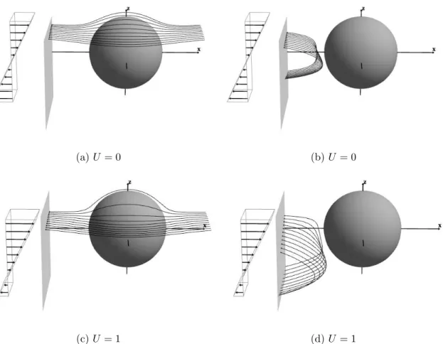
2.8 Fluid particle trajectories passing the sphere or blocked. . . 43

2.9 Trajectories of fluid particles starting from those black dots when U = 3. 44 2.10 Bifurcation diagram below the sphere. . . 46

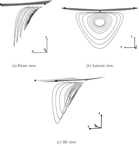
2.11 Circulation near the elliptical and hyperbolic critical points. . . 54

2.12 Different views of circulation below the sphere. . . 55

2.13 Closed and open streamlines below the sphere. . . 55

2.14 Streamlines in the symmetry plane when shear flow past a freely rotating sphere. . . 57

3.1 A linear shear flow past a fixed prolate spheroid. . . 60

3.2 Streamlines in the symmetry plane for a linear shear past an upright spheroid. . . 63

3.3 “Footprint” of stagnation surfaces on the spheroid surface from different viewpoints. . . 64

3.4 Blocked streamlines near the separation surface. . . 70

(14)

3.6 Cross sections of the blocked region at x=−5 fixed. . . 73

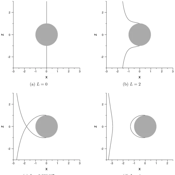
4.1 Trajectories in the x-y symmetry plane. . . 78

4.2 3D view o f trajectories in the x-y symmetry plane whenL >2. . . 79

4.3 Critical points in the flow when a fixed sphere is embedded in a rotating background flow. . . 81

4.4 Same as Figure 4.3 but for the case of the sphere freely self-rotating in a rotating background flow (γ =−1). . . 83

4.5 Trajectories in the x-y symmetry plane with a freely-rotating sphere. . 84

4.6 Trajectories out of the x-y symmetry plane when the sphere is freely rotating and L= 4. . . 84

4.7 Same as Figure 4.3 and 4.4 but with a unit sphere self-rotating in an opposite direction with respect to the background flow (γ = 1). . . 86

4.8 Trajectories in the x-y symmetry plane when the sphere is self-rotating in an opposite direction with respect to the background flow. . . 87

4.9 Trajectories out of the x-y symmetry plane when the sphere is self-rotating in an opposite direction with respect to the background flow. . 87

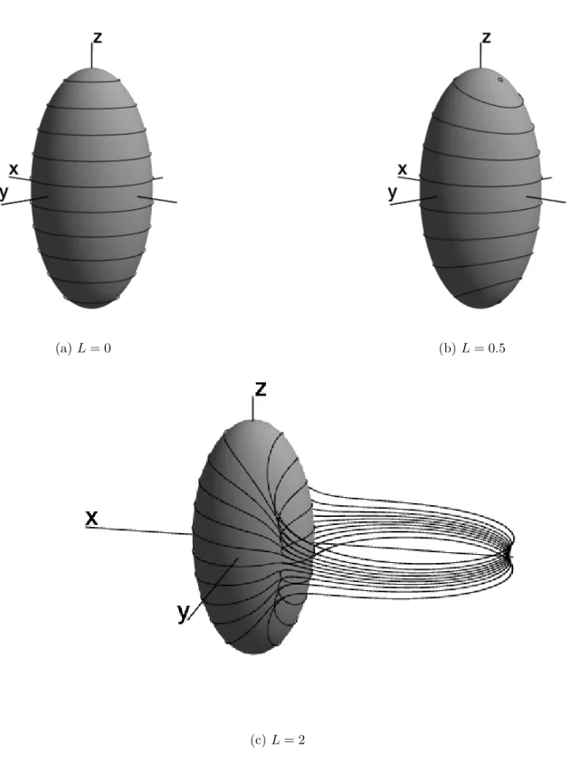
4.10 A rotating flow past an upright spheroid withω= 1 and different values of L. . . 93

4.11 Fluid particle trajectories in the rotation flow past a tilted spheroid. . . 94

4.12 A fluid particle trajectory in the rotation flow past a tilted spheroid. . . 95

5.1 Setup of the tank, cameras, diffusers, and lighting. . . 99

5.2 Configuration of a bent rod sweeping out an upright cone. . . 99

5.3 Bent pins used in our experiments. . . 100

5.4 The main calibration toolbox window. . . 102

(15)

5.7 Extrinsic parameters. . . 105

5.8 Extrinsic parameters with the camera on. . . 105

5.9 Reprojection error. . . 106

5.10 The stereo calibration window. . . 107

5.11 Extrinsic parameters for the 3D stereo calibration. . . 108

5.12 Snapshot of tracking. . . 109

6.1 A fluid particle trajectory within 10 revolutions of the straight rod sweep-ing out an upright cone. . . 119

6.2 Fluid particle trajectories. . . 120

6.3 Fluid particle trajectories. . . 122

6.4 Similar to Figure 6.3 but with the tilt angle λ= π₆. . . 123

6.5 Open fluid particle trajectories. . . 124

6.6 Positions of the rod from tracked data. . . 130

6.7 Tracked angles for the experiment of Figure 6.6. . . 131

6.8 Experimental trajectories compare to numerical trajectories. . . 133

6.9 Different numerical trajectories. . . 134

7.1 Configuration of a bent rod sweeping out an upright cone. . . 136

7.2 Four extreme statuses of the cone. . . 136

7.3 A short-time fluid particle trajectory created by a bent rod sweeping out an upright cone above a no-slip plane. . . 140

7.4 Trajectory generated by spinning a bent rod vs a straight rod. . . 141

7.5 A long-time particle trajectory in the lab frame. . . 142

7.6 The cross section of the trajectory in Figure 7.5 in the x-z plane. . . . 142

(16)

7.8 Poincar´e map of fluid particle trajectories with a straight rod. . . 143 7.9 Time to complete a full torus. . . 145 7.10 Poincar´e maps for buoyant particles. . . 147 7.11 The torque at the origin as functions of the scooping angleβ or the cone

angle κ. . . 153 7.12 Comparisons of each component of the torque with different values of

the cone angle κ. . . 153 7.13 A torus captured with red dye and a torus created with the model in the

lab frame. . . 155 7.14 An experimental trajectory tracked from two camera-views in pixel

co-ordinates. . . 156 7.15 Tracked trajectories when the rod is scooping and rotating clockwise

from top view (opposite to the motion for Figure 7.14). . . 156 7.16 Comparison of the experimental trajectory with a numerical one. . . . 157 7.17 Long-time comparison of the experimental trajectory (red) with the

nu-merical trajectory (blue) in Figure 7.16. . . 158 7.18 Comparison of the Poincar´e map of experimental and numerical

trajec-tories. . . 158 7.19 Tracked trajectories in the silicone oil when the rod is scooping and

rotating clockwise from the top view. . . 159 7.20 3D tracked trajectory and a few positions of the rod . . . 159 7.21 Tracked trajectories in silicone oil when the rod is scooping and rotating

clockwise from top view. . . 160 7.22 Comparison of numerical trajectory with experimental trajectory. . . . 161 7.23 Fluid particle trajectories . . . 164 7.24 Fluid particle trajectories with a straight rod sweeping out a double cone

in free space. . . 165

(17)

8.2 Configuration of the periodic motion of the slender body in the x-y plane.168

8.3 Two groups of fluid particle trajectories. . . 172

8.4 Three groups of fluid particle trajectories with longitudinal translation of the body. . . 174

8.5 Fluid particle trajectories in the flow introduced by the counter-clockwise rotation of the slender body. . . 177

8.6 Fluid particle trajectories within one counter-clockwise rotation of the body. . . 178

8.7 Numerical trajectories in the velocity field introduced by the anti-clockwise rotation of the slender body with `= 0.5,U = 1 andT1 = 2. . . 178

8.9 Two groups of fluid particle trajectories and part of imprints of the periodic motion of the slender body. . . 182

8.8 Fluid particle trajectories within one period. . . 182

8.10 Two groups of fluid particle trajectories in the x-y plane. . . 183

8.11 Contour plot for exact solution (8.17) of the far-field trajectory. . . 186

8.12 Contour plot for the exact solution (8.18) of the far-field trajectory. . . 189

8.13 Contour plot for (8.20). . . 191

8.14 Contour plot for exact solution (8.20) (purple) of the far-field trajectory and the averaged trajectory from (8.23) (green). . . 196

8.15 Zoom in on Figure 8.14. . . 196

B.1 Fluid particle trajectories. . . 234

B.2 Compare the exact fluid particle trajectories (black) with the slender body approximation (red) with = 1 log(2_r`). . . 235

B.3 Similar to Figure B.2, but with the initial positionx=−0.7,y= 0, and z = 0.4 . . . 235

(18)

B.5 Trajectories with different definitions of in the slender body theory. . 236

C.1 Comparison of fluid particle trajectories. . . 249

G.1 Comparison of terminal velocity of a sphere with a horizontal oblate spheroid . . . 307

G.2 The ratio of terminal velocitiesfb(1, b) in (G.9) . . . 308

G.3 Ratio fa(1, a) in (G.10) . . . 309

G.4 A sphere vs a slender body. . . 312

G.5 Coefficients in the terminal velocities of one single sphere vs two spheres. 317 G.6 The distance between centers of two unequal spheres while the small sphere above the large sphere. . . 322

G.7 The distance between centers of two unequal spheres while the small sphere below the large sphere. . . 322

(19)

List of Tables

2.1 Critical points in the interior of the flow in the x= 0 plane and

stream-lines in the y= 0 symmetry plane. . . 52

2.2 Continue of Table 2.1. . . 53

5.1 Physical properties of Karo light corn syrup. . . 101

5.2 Physical properties of Silicone Oil 12500 cst. . . 101

(20)

Chapter 1 Introduction: basic concepts,

methodology and organization

Studies of highly viscous flows past rigid obstacles and fluid flows induced by rigid bodies with small spatial scales are fundamental in fluid mechanics. These flows play an important role in particle entrainment, sediment transport, fluidic mixing, micro-organism locomotion and many other areas of geophysical and biophysical interests. In these studies, an important class of problems concerns scales where inertia plays a subdominant role to viscous forces, which is the case for many biophysical applications. The Stokes approximation becomes relevant in such cases, despite its limitations in governing fluid motion far from the body. Numerous studies have addressed these Stokes problems in the literature.

(21)

a sphere does not exist, known as Whitehead’s paradox [24]. Another version of the Stokes paradox of this 3D flow is reflected on the energy carried by the sphere or the drifting volume if we consider the flow at rest and the sphere is moving with a constant velocity. Oseen correction of uniform flow past a cylinder or sphere has already been well studied [24]. Using the matched asymptotic expansions, uniform flow past an elliptic cylinder has also been studied by Shintani et al. [68].

For a linear shear flow past an infinite cylinder, the velocity field and stream function can be found in Robertson & Acrivos [65], Poe & Acrivos [62], Kossack & Acrivos [42], and Chwang & Wu [19], and the Oseen correction for this 2D flow is derived by Bretherton [11]. In three-dimension, a general solution, the velocity field of an ellipsoid immersed in a linear Stokes flow, can be found back to Jefferey [36]. For a linear shear flow past a sphere, Saffman [66] worked out the Oseen correction for the force acting on the sphere instead of the usual stream functions. The force is governed by one ODE for this 3D flow. A good review is referred to Leal [45]. For most studies about these Stokes flow past a rigid obstacle [44, 22, 47, 41], the focus is the velocity field, the force acting on the flow [66], and sometimes the motion of the suspension in the fluid [36].

Despite the long history of research in Stokes flows, considerable attention to the Stokes flow is continually drawn due to its medical, micro-biological and geological applications. Studies of these applications can lead to better medical approaches for many aliments, better strategies of environmental issues, and deep understanding of the nature of life in the low Reynolds number regime [55], [26] [34]. For these appli-cations, not only the flow motion but also the structure of the flow plays important roles to completely understand the properties of the flow. Understanding of the flow patterns for the fundamental problems will help to predict the streamlines of flow in more complicated geometries.

(22)

investigated the flow from Lagrangian viewpoint, which is effective to show the flow structure. Therefore, this thesis focuses on the structure and interaction of the flow in the Lagrangian viewpoint. If the flow is 2D, a single valued continuous stream function can be assumed to find the streamlines. For uniform flow past a sphere in 3D, due to the axis symmetry, the flow can reduce to a 2D flow in the spherical coordinates. Jeffrey & Sherwood [37] have studied the streamline pattern for 2D Stokes shear flow around a rotating cylinder, where the flow is governed by one stream function. For a linear shear flow or rotating flow past a sphere or spheroid, the flow is fully 3D, which is much more complicated and 3D Oseen correction is extremely difficult. Acrivos’ group [1, 65, 42, 62] has studied the shear flow past a sphere experimentally and numerically. Cox, Zia & Mason [23] reported the streamline functions in integral form with a freely rotating sphere in a linear shear background flow. Beyond the Stokes regime, a few papers [72] [57] studied the flow structure numerically, considering the inertial effect for this flow. As we know, there is no report about the stream functions of a linear shear flow past a fixed sphere in the literature.

We study the flow problems with the singularity method seen in Chwang & Wu [19], Kim & Karrila [41], Pozrikidis [63], and Leal [47]. This method has been used widely in research and is especially suitable for these Stokes’ problems with regular or complicated boundary geometries. The pioneering work about the singularity method can be tracked back to Lorentz [51], Oseen [60], and Burges [13] as Chwang & Wu cited [19] (see a review [50]). The vital components for this method are to identify the type of singularities, determine the distribution and strength of the singularity, and construct the velocity eventually. The singularities are usually distributed inside the obstacle, so that the resulted velocity field is regular.

(23)

integrate and obtain the trajectory equation of fluid particles. An interesting blocking phenomenon, which is reported by Poe & Acrivos [62], Chwang & Wu [19] and Jeffery & Sherwood [37] in 2D, is observed with fully 3D shear flow past a sphere or spheroid. Through careful study, new phenomena of Stokes flow are documented.

Inside the framework of the singularity method, the slender body theory is a method-ology used to take advantage of the slenderness of the body to obtain an approximation to a field surrounding it. The slender body theory has been refined by numerous authors from Batchelor [3], Cox [21] to Johnson [38]. With higher order singularities, Johnson [38] has improved the velocity to an error term of O(2) by matching asymptotics (is the slenderness parameter). Also, Blake [5] introduced the image system to handle the no-slip boundary condition on a flat plane.

By applying both the slender body theory and the image method, the second part of this thesis reports the study of the flow induced by a slender body sweeping out a cone. This study is motivated by the campus-wide Virtual Lung Project [55, 48] at the University of North Carolina at Chapel Hill, and other biological applications, for example, the flow induced by nodal cilia [12]. Motion of nodal cilia has been found playing an important role in the left-right symmetry breaking at the early stage of the mammal embryos [58, 69, 16]. We model the cilia-induced flow in the Stokes regime with the slender-body theory and imitate the rotary motion of an isolated cilium by spinning a slender bent rod in highly viscous fluid. With the help of modern visualization tools, we also perform stereoscopic fully three-dimensional experiments and reconstruct 3D Lagrangian trajectories to compare with our theoretical predictions.

(24)

equations when the sphere’s center is in the zero-velocity plane (see the first case in Figure 2.1). In particular, we study in detail the stagnation points with their associated surfaces, as these provide the framework for the blocked region geometry, and the mode of divergence of the blocked regions’ cross-sectional area is calculated. Then, we turn to the second case shown in Figure 2.1, when the center of the sphere is out of the zero-velocity plane of the primary shear. Numerical results demonstrate the persistence of the blocked regions. Complicated global bifurcations are found analytically in the flow field with special ratios related to the shear rate, the radius of the sphere, and the distance from the zero velocity plane of the primary shear to the sphere’s center. Furthermore, we show information about the linear shear flow past a freely rotating sphere. Analytical particle trajectory formulas are obtained similarly. There are closed orbits in the flow and the height of the closed orbit near the sphere is convergent.

(25)

of the sphere, new phenomena appear in the structure of the flow. The analytical and numerical results for rotating flow past a spheroid are presented at the end of this chapter. When a spheroid is tilted in a direction tangential to the rotation background flow, fluid transport is observed.

(26)

discussed. In Chapter 8, a swimming related application of slender body theory is documented. We focus on the flow induced by a periodic motion of a slender body.

(27)

Part I

Theoretical studies of linear shear

or rotation Stokes flow past a

(28)

Chapter 2 Lagrangian blocking in highly

viscous shear flows past a sphere

Fluid flow over a rigid body in the Stokes’ regime is a fundamental problem and has received attention over more than a century. While the case of uniform flows and its ensuing far-field paradoxes in two and three dimensions are well known, features associ-ated with (spatially) non-uniform fluid flows at the far field have received comparatively less attention in the literature.

(29)

linear shear. (In this thesis, we use the terminology “disk” to refer to an infinitely long cylinder whose axis is perpendicular to the background stream, i.e. an inherently two-dimensional setup). These authors noted an interesting blocking phenomenon which was observed numerically and experimentally by Acrivos’ group [65, 62]. This blocking behaviour is a strong modification of the particle trajectories from situations without and with a fixed disk: in the absence of the body, particles are swept by the shear flow on straight horizontal lines, never crossing the zero-velocity horizontal line. When the disk is placed into the flow, two regions of fluid emerge in which particles cross the zero-velocity line as they approach the disc in either forward or backward time. Parti-cles initially within these regions are confined to them, and will never pass through the vertical line through the disk’s center orthogonal to the background shear flow. One of the focuses of this chapter is to analyse this kind of phenomenon in more general 3D flows associated with a sphere or spheroid.

Generally, the regions where blockage occurs are bounded by separation ‘stream-surfaces’. In the 2D case involving linear shear flow past a disk, the height of these separation streamlines becomes infinite far from the disk, an effect which was observed by Bretherton [11] and Chwang & Wu [19] and was conjectured not to persist in 3D shear flow past a fixed sphere. This case appears to not have been studied in detail, although particle trajectories are sketched in the symmetry plane by Robertson & Acrivos [65] and Leal [47].

(30)

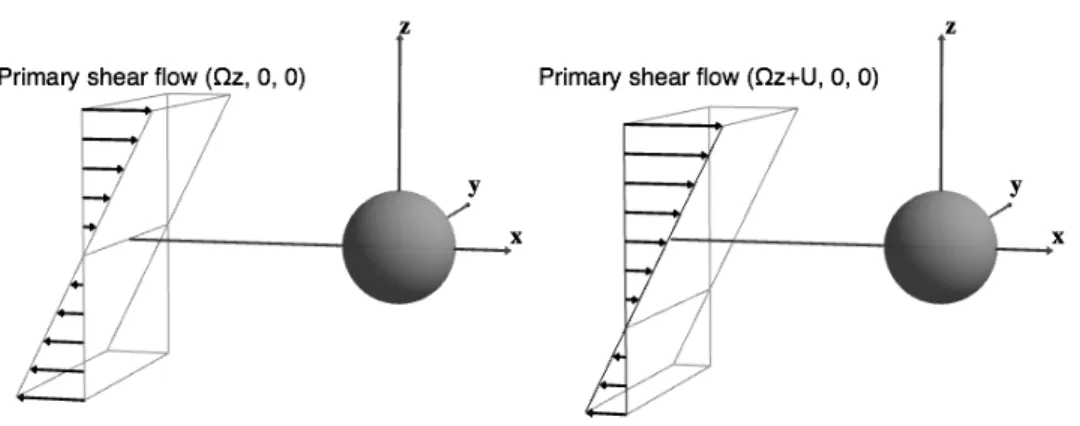
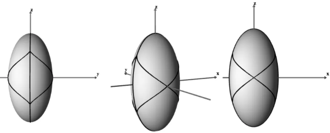
Figure 2.1: Flow past a fixed sphere x2 ₊_y2 ₊_z2 ₌ _a2_{. Without lost of generality,}

assume Ω≥0 and U ≥0.

(31)

2.1 Formulation of problem

We study the motion of an unbounded linear shear flowU= Ωzex+Uex of constant densityρ and dynamic viscosity µ, past a fixed sphere

x2+y2+z2 =a2. (2.1)

Since the fluid is incompressible, the continuity equation is

divu= 0, (2.2)

where u is the fluid velocity. In this thesis, we assume that the inertial terms in the Navier-Stokes equations can be neglected. Thus, the equations of motion are

µ∇2u=∇p, (2.3)

where p denotes the fluid pressure. The condition for (2.3) to hold is that Re = Ωa2_ρ/µ_{1. The boundary conditions are that} _u_{= 0 on the solid boundary, and} _u_is

asymptotic to the basic shear flow at large distances from the rigid body.

Schematics of the problems are shown in Figure 2.1. Case 1 on the left is the shear flow Ωzex past a fixed sphere at the origin. Case 2 on the right is the shear Ωzex+Uex past the sphere, where the sphere’s center is out of the zero-velocity plane of the background shear.

(32)

shear is

u = Ω

zex− 5a3

6 3xzx

r5 +

a3

2

ey×x

r3 −

a5 6∇ ∂2 ∂x∂z 1 r +U

ex− 3a

4

ex

r +

(ex·x)x

r3 + a 3 4 ∇ ∂ ∂x 1 r , (2.4)

wherex= (x, y, z),r =|x|=px2₊_y2 ₊_z2_, _e

x,ey and ey are unit vectors along x,y, and z direction, respectively. The force acting on the fixed sphere is F= 6πµ Uex and the torque at the origin isT=−4πµΩa3ez [19].

Letx0 = x_a, u0 = _au_Ω andU0 = _aU_Ω, nondimensionalizing the equations (dropping the primes), the non-dimensional velocity field is

u = zex− 5 2

xzx

r5 +

ey×x 2r3 −

1 6∇ ∂2 ∂x∂z 1 r +U

ex− 3 4

ex

r +

(ex·x)x

r3 + 1 4∇ ∂ ∂x 1 r . (2.5)

From now on, we use the non-dimensional variables unless stated otherwise.

2.2 Linear shear flow past a sphere whose center

is in the zero-velocity plane of the background

flow

(33)

analytically calculate the stagnation points, the 3D separatrix, and the measurement of blocking regions. Additionally, we analyze the structure of the flow near the sphere. For this case, the center of the sphere is in the zero-velocity plane of the background, and the velocity field is a simplified form of equation (2.5)

u=zex− 5 2

xzx

r5 +

ey×x 2r3 −

1 6∇

∂2 ∂x∂z

1

r. (2.6)

2.2.1 Exact quadrature formulae for the fluid particle

trajec-tories

Here, streamlines may be constructed as the intersection of two stream surfaces for a 3D flow. Of course, it is not always possible to find explicit formulas of streamlines for a flow field, and we show how particle trajectories may be computed in closed form for the complex flow under study in this chapter.

Based on the special geometry of this problem, we change the coordinates from rectangular coordinates to spherical coordinates (r, φ, θ). Using the explicit fluid flow, we may immediately write the particle trajectory equations in spherical coordinates as:



    

    

dr

dt = cos(θ) sin(2φ)

3−5r2₊₂_r5

4r4 ,

dθ

dt = sin(θ) cot(φ)

1+r2₋₂_r5

2r5 ,

dφ

dt = cos(θ)

cos(2φ)₍r5₋₁₎₊_r5₋_r2

2r5 ,

(2.7)

wherer=px2₊_y2₊_z2₍₁_≤_{r <}_∞),_φ_{= arccos} z r

(0≤φ≤π), andθ = arctan y_x (0≤θ ≤2π).

(34)

radius r as a new independent variable giving a system for dφ_dr and dθ_dr:

dθ dr =

(1 +r2₋₂_r5_{) tan(}_θ₎

(3r−5r3 _{+ 2}_r6_{) sin}2₍_φ₎,

dφ dr =

−r2+r5+ (r5−1) cos(2φ)

r(3−5r2 _{+ 2}_r5_{) cos(}_φ_{) sin(}_φ₎.

Next, changing the variable y = rsin(θ) sin(φ) and taking the derivative of y with respect tor, yields:

dy

dr = sin(θ) sin(φ) +rcos(θ) sin(φ) dθ

dr +rsin(θ) cos(φ) dφ dr.

Substituting dθ_dr and dφ_dr into the above equation and replacing sin(θ) sin(φ) with y_r, we get

dy dr =

−5(1 +r) sin(θ) sin(φ) (r−1)(3 + 6r+ 4r2_{+ 2}_r3₎ =

−5(1 +r)y

r(r−1)(3 + 6r+ 4r2_{+ 2}_r3₎. (2.8)

Similarly, take derivative of z =rcos(φ) with respect to r and substitute dφ_dr into the resulting formula,

dz

dr = cos(φ)−rsin(φ) dφ dr =

(1 +r)(3 + 5(2 cos2(φ)−1)) (6 + 6r−4r2₋₄_r3₋₄_r4_{) cos(}_φ₎.

Replacing cos(φ) withz/r, the above equation becomes

dz dr =

(r+ 1) (r2−5z2)

r(r−1) (3 + 6r+ 4r2_{+ 2}_r3₎_z. (2.9)

The obtained ODEs dy_dr and dz_dr decouple.

(35)

solution is,

y3 = C1

r5

(r−1)2_{(3 + 6}_r_{+ 4}_r2_{+ 2}_r3₎. (2.10)

The ODE in equation (2.9) is not exact, and hence not immediately separable, nonethe-less an integrating factor may be found. We rewrite it as

(1 +r)(r2₋₅_z2₎

(r−1)r(3 + 6r+ 4r2_{+ 2}_r3₎dr−zdz = 0.

Notice that multiplying this equations by the integrating factor (3−5r2+2r5)

2 3

r103

yields an exact equation which is solved in closed integral form:

Z 1_r

(1 +s)(1−s)13

(2 + 4s+ 6s2_{+ 3}_s3₎13

ds−(3−5r

2_{+ 2}_r5₎23

2r103

z2 =C2. (2.11)

HereC1 and C2 are constants determined by the initial values r0,y0, and z0.

Equations (2.10) and (2.11) describe the fluid particle trajectories. If r0 6= 1, (2.11)

can be rewritten to read:

z2 = 2r

10 3

(3−5r2_{+ 2}_r5₎23

Z _r1

0 1

r

(1 +s)(1−s) (2−5s3_{+ 3}_s5₎13

ds+z₀2

r r0

10₃

3−5r₀2+ 2r5₀

3−5r2_{+ 2}_r5

2₃

. (2.12)

This equation expresses the height, z, of the fluid particle trajectory in terms of r. These trajectory equations provide rigorous tools to study the blocking phenomenon.

2.2.2 Blocking phenomenon

(36)

particles released in the shear flow (starting, say, above thez = 0 plane) will be swept from large negative x values, to large positive x values as time progresses. However, when the fixed, solid sphere is introduced into the flow, a large measure of particle trajectories lose this streaming property. Namely, blocked particles starting with large negative x values do not pass the sphere as time progresses, but rather, limit back to large negative x values as time progresses. The regions where this behavior occurs in three dimensional space are defined to be the “blocked regions” of the flow. See Figure 2 which depicts this blocking region when the flow is restricted to the two dimensional symmetry plane. We note that this type of behavior has been observed for the case of an infinitely long cylinder immersed in a linear shear flow by Chwang & Wu [19]; however, they conjectured that this behavior would not persist for situations involving a sphere (instead of a cylinder). Here, we show that in fact for the case of the sphere, the blocking region persists, and moreover, we analytically compute the geometry of this region, and show that it has infinite cross-sectional area. With the exact, closed form expressions for the particle trajectories given in equations (2.10) and (2.12), we may proceed directly to computing the geometry of the blocked regions.

Blocking phenomenon in the y= 0 symmetry plane

In the y= 0 plane, the velocity field is

u(x,0, z) = z

1− 1 2r3 −

5x2

2r5 −

z2₋₄_x2

2r7

, v(x,0, z) = 0,

w(x,0, z) = x

1 2r3 −

5z2

2r5 −

x2₋₄_z2

2r7

,

and r = px2₊_y2₊_z2 ₌ √_x2₊_z2_{. Notice that one velocity component} _v _vanishes.

(37)

Figure 2.2: Streamlines in the y = 0 plane with the linear shear flow zex past a fixed sphere. The four black points on the sphere are stagnation points in this symmetry plane. Note that the separatrix height limits to approximately 0.88207 and is rigorously less than unity.

trajectory. Fluid particles in this plane are thus described by the closed integral formula equation (2.12) with r2₀ = x2₀ +z₀2 and r2 = x2 +z2. The streamlines in the y = 0 symmetry plane shown in Figure 2.2 explicitly depict the blocking region. The fully 3D structure of the blocking region will be described below.

The four dots on the sphere in Figure 2.2 are stagnation points. They are (x, y, z) = (±_√2

5,0,± 1

√

5) in rectangular coordinates. Two other stagnation points on the sphere

(38)

From figure 2.2, it is clear that there are blocking regions. For example, the flow is separated by the stagnation line in the second quadrant. Below that stagnation line the flow is trapped on the left side of the sphere.

It is worth comparing this case with that of the analogous 2D flow: For the 2D flow in the case of an infinitely long cylinder immersed in a linear shear flow with the cylinder axis perpendicular to the lines of constant shear [37], the stream function is

φ(x, z) = 1 2z

2

1− 1

r2

2

+1 4

1− 1

r2

− 1 2logr

see Chwang & Wu [19] for more details. Here r2 ₌ _x2 ₊_z2_{, and the radius of the}

cylinder is unity. The stagnation points on the cylinder are (±

√

3 2 ,±

1

2). Notice that

the separatrix is totally explicit in this case. Moreover, as x → ±∞, the height |z| of separatrix goes to∞. This peculiar behavior is in some sense similar to the well-known Stokes Paradox in 2D uniform flow past a cylinder. Our results below show that the limiting height of the separatrix is finite in the case involving a fixed, rigid sphere, in sharp contrast with the 2D case.

Blocking phenomenon off the y= 0 plane

By continuity, it is expected that the blocking phenomenon extends outside the

(39)

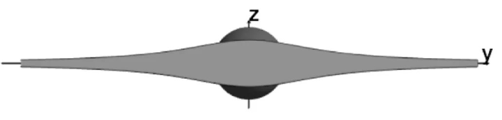
Figure 2.3: Separation surfaces generated by separatrix lines in the flow.

Recall equations (2.10) and (2.12) with initial value (x0, y0, z0):

y=y0

r53 (r₀−1) 2

3 _{(3 + 6}_r

0+ 4r20+ 2r30)

1 3

r

5 3

0(r−1)

2

3 (3 + 6r+ 4r2+ 2r3) 1 3

,

z2 = 2r

10 3

(3−5r2_{+ 2}_r5₎23

Z _r1

0

1

r

(1 +s)(1−s)13

(2 + 4s+ 6s2_{+ 3}_s3₎13

ds+z₀2r

10 3

r

10 3

0

3−5r2 0+ 2r50

3−5r2_{+ 2}_r5

23

,

where r0 =

p

x2

0+y02+z02. Particle trajectories are determined by simultaneously

solving (intersecting these surfaces) these equations to obtain a curve relating (x, y, z). Figure 2.3 shows the separation surfaces in the flow. As shown in this figure, there is a region off thex-z plane between the separation surfaces, where the flow is blocked. The vertical plane in this figure shows the cross section of the blocking region. The cross-sectional area in the limit of x→ ±∞will be discussed in subsection 2.2.6.

(40)

(a) Streamlines close to the sphere. (b) Zoom in the cube near they-axis. Figure 2.4: Streamlines on separation surfaces close to the sphere.

the rigid sphere. From Figure 2.4b, it is easy to see that they are hyperbolic critical points.

2.2.3 Stagnation points on the sphere

Since all points on a solid boundary are fixed points of the flow, special care is needed to define stagnation points which reside on a solid boundary. This degeneracy on solid boundaries may be split by computing those points on the boundary for which the linearization of the velocity vector field vanishes. These will define the stagnation points on the rigid boundary. Streamlines in the fluid which end at any stagnation point (whether in the fluid or on the boundary) are referred to as stagnation lines. Stagnation lines ending on the boundary are not necessarily perpendicular to the no-slip, rigid boundary. For 2D flow, the angle between the stagnation line and the rigid surface can be computed, as seen in Pozrikidis [63].

(41)

are linearized with respect to radiusr at 1, the expansions are

dr

dt = O((r−1)

2₎_,

dθ

dt = −4 cot(φ) sin(θ)(r−1) +O((r−1)

2₎_,

dφ dt =

3 + 5 cos(2φ)

2 cos(θ)(r−1) +O((r−1)

2₎_.

After rescaling timeτ =t(r−1) and neglecting the higher order, we reduce the ODE system to

dr

dτ = 0, dθ

dτ = −4 cot(φ) sin(θ), (2.13) dφ

dτ =

3 + 5 cos(2φ)

2 cos(θ).

The steady state of the above ODE system provides the stagnation points, yielding the following conditions:

cot(φ) sin(θ) = 0, 2 cos(θ)(5 cos2(φ)−1) = 0.

Since 1≤r ≤ ∞, 0≤φ≤π, 0≤θ < 2π, six stagnation points on the sphere are

r = 1,



 

 

θ = 0, π, φ = arccos√1

5

,arccos−_√1 5

;

and



 

 

θ = π₂,3₂π;

φ = π₂

.

Rewritten in rectangular coordinates, these points are located at

(0,±1,0),

±√2 5,0,±

1 √ 5

(2.14)

(42)

The rescaled velocity field provides an imprint of the particle trajectory pattern just off the sphere surface which mathematically reduces to heteroclinic connections between the stagnation points. These connections can be found from the ODE system (2.13),

dθ dφ =−

8 cot(φ) tan(θ) 3 + 5 cos(2φ) ,

and the solution is

sin(θ)2 =C4 cos

2₍_φ₎₋_sin2₍_φ₎

sin2(φ) =C

5 cos2(φ)−1

sin2(φ) , (2.15) whereC is a constant depending on the initial value of r,θ, andφ. Whenr= 1, using the stagnation points as initial conditions, we get the equation of the trajectories on the sphere in rectangular coordinates:

(x, y, z) =±2 cos(φ),±p1−5 cos2₍_φ₎_,_±_cos(_φ₎_, _arccos₁_/√₅_{< φ < π/}₂_.

(43)

Figure 2.5: “Footprint” of stagnation surfaces on the sphere.

2.2.4 Critical points on the

y

-axis

Beside the stationary points on the surface of the sphere, we further remark that the entire y-axis exterior to the sphere is a line of fixed points. For finitey values along this line, they are hyperbolic points (in thex-z plane) with orientation depending upon the distance from the sphere. Infinitely far from the sphere along the y-axis, these fixed points lose their hyperbolic structure, with the flow becoming a simple shear flow (the background flow). In this limit, the orientation angle tends to zero. In the opposite limit, approaching the sphere, this line of hyperbolic points tend to the higher order hyperbolic fixed point on the sphere, with the orientation angle depicted by the geodesic curves in Figure 2.5, with tangent value 4/3, which can also be verified by the local analysis near the critical points on the y-axis.

(44)

-15 -10 -5 5 10 15 x -1.0 -0.5 0.5 1.0 z

Figure 2.6: Eigenvectors of matrix A at x= 0, y0 = 5, z = 0.

a point on the y-axis (0, y0,0), the linearized velocity field is

      dx dt dy dt dz dt       =      

0 0 2y50−y20−1

2y05

0 0 0

y2 0−1

2y5

0 0 0

            x y z       .

This shows that the flow near (0, y0,0) can be reviewed as 2D flow in the x-z plane,

   dx dt dz dt   =   

0 2y50−y20−1

2y5 0

y2 0−1

2y5 0 0       x z   ≡A

   x z   .

Eigenvalues of matrix A are ±(y0−1) q

(1+y0)(1+y0+2y20+2y03+2y04)

2y5

0 , and the corresponding

eigenvectors are



± s

1 +y0+ 2y02+ 2y03+ 2y40

1 +y0

,1



.

Figure 2.6 shows the eigenvectors at the point (0,5,0). As y0 → ∞, the angle between

the eigenvectors goes to zero. When y0 → 1, the eigenvectors are (±2,1), i.e., the

(45)

2.2.5 Stagnation lines

The precise mathematical definition of the blocking region requires some care to set up. Clearly, the unblocking and blocking regions are divided by the separation surfaces created by stagnation lines in the interior of the fluid as depicted in Figures 2.2 and 2.3. These regions may be succinctly defined as follows: We define the set of unblocked trajectories to be the set of initial points whose particle trajectories intersect thex= 0 plane off of the y-axis in finite or infinite time. This set of points is topologically open. The complement of this set (thus closed), we define to be the blocking region. Notice that the boundary of this set defines the separation surface. This connected surface contains the separating surface in the fluid, the y-axis, and the sphere surface.

To calculate this separation surface, we first identify the stagnation lines using the explicit formulae for the trajectory equations given in (2.10) and (2.12), then study their properties on and off the y = 0 symmetry plane. Through this analysis, we will prove that the height |z| of stagnation lines is finite as x→ ±∞ and y fixed.

Stagnation lines in the y= 0 symmetry plane

Since one velocity component vanishes in this plane, streamlines are only governed by equation (2.12)

z2 = 1

3 2r5 −

5 2r3 + 1

2₃ 

 Z 1_r

(1 +s)(1−s)13

1 + 2s+ 3s2₊3 2s

31₃

ds+C



,

whereC is determined by the initial value (x0,0, z0).

As we know from the previous subsection, four stagnation points on the sphere in this symmetry plane are (±_√2

5,0,± 1

√

(46)

get the equation of the stagnation line in this plane

z2 = 1

3

2r5 − ₂5_r3 + 1

2₃ Z 1

1

r

(1 +s)(1−s)13

1 + 2s+ 3s2₊3 2s

31₃

ds.

A few remarks regarding this stagnation line may be made. First, the height of the stagnation line, |z|, is bounded. This is easily seen by replacing the denominator in the integrand by unity, and evaluating the integral. This gives a constant slightly bigger than the unit sphere radius. Second, this bound may be improved substantially through dividing the integral into subintervals and further integrand estimates. In fact, this ultimately establishes very tight upper and lower bounds for the limiting height value of the stagnation line in the limit x→ ∞. This upper bound is less than unity, with value 0.8831, and the lower bound is 0.8811. Numerically, we find

|zmax| ≈ 0.88207 asr → ∞.

Integral estimates for the height of the stagnation line

In the y = 0 symmetry plane, the height of the stagnation lines |z| satisfies the following equation

z2 = 1

3 2r5 −

5 2r3 + 1

2/3 Z 1

1

r

(1 +s)(1−s)1/3

1 + 2s+ 3s2₊3 2s3

1/3 ds.

Let= 1_r, then

z2 = 1

3 25−

5 23+ 1

2/3 Z 1

(1 +s)(1−s)1/3

1 + 2s+ 3s2₊ 3 2s3

1/3ds.

(47)

When < ₁₀1,

R1

(1+s)(1−s)1/3

(1+2s+3s2₊3 2s3)

1/3 ds < z

2 _<_{1 +} 53

3

R1

(1+s)(1−s)1/3

(1+2s+3s2₊3 2s3)

1/3 ds <

601 600

R1

(1+s)(1−s)1/3

(1+2s+3s2₊3 2s3)

1/3 ds <

601 600

R1

0

(1+s)(1−s)1/3

(1+2s+3s2₊3 2s3)

1/3ds, (2.16)

since 1< 1

(3 25−

5 23+1)

2/3 <1 +

53

3 < 601 600.

When < ₁₀₀₀1 ,

Z 1

(1 +s)(1−s)1/3

1 + 2s+ 3s2₊ 3 2s3

1/3 ds > Z 1

0

(1 +s)(1−s)1/3

1 + 2s+ 3s2₊ 3 2s3

1/3 ds−

>

Z 1

0

(1 +s)(1−s)1/3

1 + 2s+ 3s2₊3 2s3

1/3 ds−

1 1000.

Substitute the above lower bound into (2.16), the height of the stagnation line |z| is bounded as

Z 1

0

(1 +s)(1−s)1/3

1 + 2s+ 3s2₊ 3 2s3

1/3 ds−

1 1000 < z

2 _< 601

600

Z 1

0

(1 +s)(1−s)1/3

1 + 2s+ 3s2₊3 2s3

1/3ds.

(2.17) Next, we break the integral interval into two subintervals [0,1₂] and [1₂,1] and estimate the integrand on each subintervals.

When 0≤s≤ 1 2,

L1 ≡

1−s2₊ 5s3

6 − 4s5

3 + 25s6

18 +

s7

2 − 55s8

18

< (1+s)(1−s)1/3

(1+2s+3s2₊3 2s3)

1/3 (2.18)

<1−s2₊ 5s3

6 − 4s5

3 + 25s6

18 +

s7

2

(48)

and when 1₂ ≤s≤1,

L2 = ₁₅2

1/3

(1−s)1/3

2 + ₁₀1(1−s)< (1+s)(1−s)1/3

(1+2s+3s2₊3 2s3)

1/3 (2.20)

< ₁₅2 1/3

(1−s)1/3h_{2 +} (1−s) 9 +

(1−s)2

81 −

347(1−s)3

10935 −

4261(1−s)4

98415

i

=H2. (2.21)

Evaluate the integrals with the lower or upper bounds in (2.18)-(2.21),

Z 1₂

0

L1ds =

1089251 2322432,

Z 1₂

0

H1ds=

121199 258048,

Z 1

1 2

L2ds=

7132/3

28051/3,

and

Z 1

1 2

H2ds=

1164154073 1528450560151/3.

Keep four decimal places and substitute these estimations into (2.17), the estimates for

z2 _{are 0}_.₇₇₆₄ _{< z}2 _< ₀_._{7799. Eventually, the bounds for the height of the stagnation}

lines far from sphere r→ ∞ are

0.8811 <|z|<0.8831.

Stagnation lines off the y= 0 symmetry plane

We next calculate the stagnation surface out of the symmetry plane. As shown in subsection 2.2.4, the set of critical points which are detached from the sphere is the

y-axis. Thus any stagnation line not in the symmetry plane must contain a unique point on the y-axis (as shown in Figure 2.3 and Figure 2.4 which demonstrate this fact). We use these critical points as the initial conditions r0 = y0 > 1, z0 = 0, and

(49)

stagnation lines lying outside of the symmetry plane

y =y0

r53 (y₀−1) 2

3 _{(3 + 6}_y

0+ 4y02+ 2y03)

1 3

y

5 3

0(r−1)

2

3 (3 + 6r+ 4r2+ 2r3) 1 3

, (2.22)

z2 = 2r

10 3

(3−5r2_{+ 2}_r5₎23

Z _y1

0 1

r

(1 +s)(1−s)13

(2 + 4s+ 6s2_{+ 3}_s3₎13

ds. (2.23)

This provides the equations for the stagnation lines out the symmetry plane.

Notice that the stagnation line in the symmetry plane terminates on the sphere at a point which is not on the y-axis. So next we investigate how the points on the separation surface close to the symmetry plane topologically connect stagnation lines intersecting the y-axis with the stagnation line in the symmetry plane. (Due to the symmetry of the flow, we only consider the case of y0 close to +1. )

Using they coordinate of the stagnation lines crossing the y-axis given in equation (2.22), with initial condition (0,1 +δ,0) (δ1), we have

y=

δ2_{(15 + 20}_δ_{+ 10}_δ2_{+ 2}_δ3₎

2(1 +δ)2

13

1− 1

r

−2₃

1 + 2

r +

3

r2 +

3 2r3

−1₃

.

The initial condition specifies a point close to (0,1,0). In the limit of r → ∞, this limits to

15 2

1₃

δ23

1 + 4₃δ+ 2₃δ2₊ 2 15δ

31₃

(1 +δ)23

,

and asδ →0, the leading order approximation is 15₂

1

3 _δ2₃_. _{This shows that the out of}

the symmetry plane stagnation line crossing the critical point (0, y0,0), which is

(50)

Figure 2.7: Light gray area is the front view of the cross section of the bounded blocking region at x=∞.

the cross-sectional area of the blocking region.

2.2.6 Cross-sectional area of the blocking region

We next study the geometry of this blocking region far from the sphere. We do this by examining its cross-sectional structure (as in Figure 2.3 and Figure 2.7).

Unfortunately, at finite distances from the body, this cross-sectional region of in-tersecting the plane x =L with the stagnation surface is not readily provided by the equations in (2.22) and (2.23) as they are parametrized by the spherical radius. Fortu-nately, we can overcome this difficulty by working withL→ ∞sincer ∼xin this limit. In this limit, the formulae in equations (2.22) and (2.23) provide (y, z) coordinates for the curves bounding the blocking region, shown for large, but finite L, in Figure 2.7). While from this figure it is clear that the heightz =z(y) will decay to zero as y → ∞, the limiting procedure yields a parametric representation (with parameter y0) for this

(51)

From the equations of the stagnation lines (2.22) and (2.23), we get

y ∼ y0

1− 1

y0

2₃

1 + 2

y0

+ 3

y2 0

+ 3 2y3

0

1₃

, (2.24)

z2 ∼

Z _y1

0

(1 +s)(1−s)13

1 + 2s+ 3s2₊3 2s3

1₃ds = (z∞)

2

, (2.25)

as r → ∞ by taking x → ∞, where z∞ > 0. Here y0, a point on the y-axis, is the

initial value in the trajectory equations for y, and z. This parametric representation for the curve z = z(y) may be viewed as an image of the y axis under the flow after infinite time, which we may use to derive an explicit expression for the cross-sectional area. To whit, the Jacobian matrix for this mapping is

dy dy0

=

1 + 3 2y5

0

− 5 2y3

0

1₃

+ 5 (1 +y0)

2y4 0

1− 1

y0

1₃

2 + _y4

0 +

6

y2 0

+_y33 0

2₃.

The area of the blocking flow is noted as A,

A

4 =

Z ∞

0

z(y)dy =

Z ∞

1

z∞(y0)

dy dy0 dy0 = Z ∞ 1 z∞

1 + 3 2y5

0

− 5 2y3

0

1₃

dy0+

Z ∞

1

z∞

5 (1 +y0)

2y4 0

1− 1

y0

1₃

2 + _y4

0 + 6 y2 0 + 3 y3 0 2₃ dy0

= Part1 + Part2.

For integral Part2, the leading order of the integrand 5(1+y0)

2y4 0

“

1−1

y0

”1

3„

2+_y4

0+ 6

y2₀+

3

y3₀

«2

3

is 5

2(2)23y3 0

as y0 → ∞. Notice that integrand in equation (2.25) is bounded. Consequently, an

upper bound for the decay of z∞ is

q

1

y0 as y0 → ∞. Thus, the integral Part2 is

(52)

We next show that integral Part1 diverges: Part1 = Z ∞ 1 z∞

1− 5 2y₀3 +

3 2y₀5

1₃

dy0 .

Substitute z∞(y0) in equation (2.25) into the integrand

Part1 =

Z ∞

1



 Z _y1

0

(1 +s)(1−s)13

1 + 2s+ 3s2₊ 3 2s

31₃

ds   1 2

1− 5 2y3

0

+ 3 2y5

0

1₃

dy0,

As y0 → ∞,

1− 5 2y3

0

+ 3 2y5

0

1₃

→1.

Using the following result to estimate the integral in the kernel (which follows directly through straightforward Taylor expansion),

Z η

0

(1 +s)(1−s)13

1 + 2s+ 3s2₊ 3 2s3

1₃ds=η−

η3

3 +O η

4

,

This establishes the following asymptotic expansion:

Z _y1

0

(1 +s)(1−s)13

1 + 2s+ 3s2₊ 3 2s3

1₃

ds∼ 1

y0

as y0 → ∞.

So, the integrand of Part1 is asymptotic toq_y1

0 asy0 → ∞. With such a decay rate the

integral R₁∞q_y1

0dy0 = ∞ is divergent. Since the integrand is sign definite, this result

shows that Part1 is divergent. Consequently, the total area of the cross-section of the blocking region is infinite when the plane x=x0 → ∞.

(53)

where it was shown that at x=∞, the cross section of the blocking region is infinite. Since the explicit, closed form formula for the area at an arbitrary distance from the sphere is not available, we study its behavior by analyzing the integrand involved here under different asymptotic limits. We will see a continuous connection between zero cross-sectional blocking area at x = 0, to diverging cross-sectional blocking area as

x→ ∞.

The separation surface is generated by the stagnation lines cross the critical points (0, y0,0) on they-axis, where|y0|>1. If we take the cross section of the blocking region

atx0, then y2+z2 =r2−x20. Based on the trajectory equation (2.22) and (2.23),

3 2

1

r5 −

5 2

1

r3 + 1

2/3

r2−x2₀ =

Z _y1

0

1

r

(s+ 1)(1−s)1/3 3

2s3+ 3s2 + 2s+ 1

1/3ds (2.26)

+y₀2

3 2 1 y5 0 − 5 2 1 y3 0 + 1 2₃ .

From the above equation, we find the mapping from r toy0 with x0 fixed. With such

a mapping, the boundary of the cross section of the blocking area can be written as parametric functions     

y = y(r(y0), y0)

z = z(r(y0), y0)

(2.27)

atx=x0 fixed. The leading order asymptotic solution to (2.26) is

r∼

q

y2

0 +x20 as y0 → ∞ and x0 fixed. (2.28)

If~a = (0, z) and~n is the outer normal direction of the cross section,

~a.~n= z(y0) dy dy0

|dy dy0|

(54)

By the Divergence theorem or Gauss’ theorem, the cross section of the blocking areaI

is an explicit integral:

I 4 = Z Ω dA = Z Ω

div~a dA=

Z

∂Ω

~a.~n ds=

Z ∞

1

z(y0)

dy dy0

dy0. (2.29)

From the asymptotic result (2.28) and several applications of the implicit function theorem to obtain derivative asymptotics (we relegate these technical details to the next subsection), we find that for finite x0, the integrand decays as √x0

2y3₀/2 when y0 → ∞, which yields a finite cross-sectional blocking area.

To study the behavior for the blocking area asx0 increases, we take the cross section

atx0 =y0, where >0 is a constant.

• When 0< < 1, from equation (2.26), we findr ∼py2

0 +y02asy0 → ∞.

Substi-tute this into the integrand for the blocking area, the integrand for the blocking area is asymptotic to _√1

2 1

y3₀/2−. When 0 < <

1

2, the integral is convergent.

Otherwise, 1₂ < < 1, the integral is divergent.

• If the cross section is taken at x0 =y0 ( ≥ 1), then r ∼

p

y2

0 +y02 as y0 → ∞.

In this case, the integrand of equation (2.29) for the blocking area decays as ₂√3

y0

with y0 → ∞.

This illustrates an unreported property about the solution of the Stokes flow but physically not observed. Since, at large distances, the characteristic length used in the Reynolds number need to be redefined, the inertia terms ignored in Navier-Stokes equation are not negligible.

If~a = 1₂(y, z), similar results are hold. Then,

~a.~n = 1 2

z(y0)_dydy

0 −y(y0)

dz dy0 r dz dy0 2

+_dydy

0

2

(55)

Similarly, by the Divergence theorem or Gauss’ theorem, the cross section of the block-ing area I is an explicit integral:

I 4 = Z Ω dA= Z Ω

div~a dA=

Z

∂Ω

~a.~n ds= 1 2

Z ∞

1

z(y0)

dy dy0

−y(y0)

dz dy0

dy0.

We find that for finite x0, the integrand decays as √x0

2y3₀/2 when y0 → ∞, and

• When 0 < < 1, from equation (2.26), the integrand for the blocking area is asymptotic to 1

8√2 1

y3₀/2−.When 0 < <

1

2, the integral is convergent. Otherwise, 1

2 < <1, the integral is divergent.

• If the cross section is taken at x0 = y0 (≥ 1), the integrand of equation (2.30)

for the blocking area decays like ₂√3

y0 as y0 → ∞, which leads to the divergence

of the integral.

Details of asymptotics of the integrand for the cross-sectional area

In this subsection, we provides the details about the decay rate of the integrand used to compute the cross-sectional area of the blocking region. When the integrand decays fast enough, the integral is convergent, which implies that the cross section of the blocking area is finite. Otherwise, the integral is divergent and the cross-sectional area of the blocking region is infinite.

The closed integral form trajectory equations (2.22) and (2.23) of the fluid particles are

y = y0



 

1− 1

y0 2 3 2 1 y3 0

+ 3_y12 0

+ 2_y1

0 + 1

1−1

r

2 ₃

2 1

r3 + 3

1

r2 + 2

1

r + 1



 

1/3

, (2.30)

z2 = 1

1 + ₂3_r5 −

5 2r3

2/3 Z _y1

0

1

r

(s+ 1)(1−s)1/3 3

2s3+ 3s2+ 2s+ 1

(56)

Substitutingy and z in the originally ODE system used to derive the trajectory equa-tions, we have

dy dr =

5 1_r + 1y

(1−r) (3 + 6r+ 4r2_{+ 2}_r3₎

= 5y0

1

r + 1

(1−r) (3 + 6r+ 4r2_{+ 2}_r3₎



 

1− 1

y0 2 3 2 1 y3 0

+ 3_y12 0

+ 2_y1

0 + 1

1− 1

r

2 ₃

2 1

r3 + 3

1

r2 + 2

1

r + 1

   1 3 (2.32) dz dr =

(1 +r) 5

r2z2−1

3 + 3r−2r2₋₂_r3₋₂_r4

r z

=

(1 +r)r 5

r2₍3 2 1

r5− 5 2

1

r3+1) 2 3 R 1 y₀ 1 r

(s+1)(1−s)13

(3

2s3+3s2+2s+1) 1

3ds−1

!

(3 + 3r−2r2₋₂_r3₋₂_r4₎

(

1

(3 2 1

r5− 5 2 1

r3+1) 2 3 R 1 y₀ 1 r

(s+1)(1−s)13

(3

2s3+3s2+2s+1) 1 3ds

)1₂

(2.33)

All these four equations are in terms ofr and y0.

If x=x0, from x2 =r2−y2−z2, we derive the following constraint

1− 5 2r3 +

3 2r5

2₃

r2−x2₀=

Z _y1

0

1

r

(s+ 1)(1−s)13

3 2s

3_{+ 3}_s2_{+ 2}_s_{+ 1}1₃ds+y

2 0

1− 5 2y3

0

+ 3 2y5

0

2₃

.

Taking implicit differentiation, we have

dr dy0

= 2y

5

0 −y02−1

y4

0(1−25r3 +₂3_r5)2/3(1− ₂5_y3 0

+ 3 2y5

0

)1/3

,

(

1−1

r

1 + 1

r

r2 ₁₋ 5 2r3 +

3 2r5

+

10y₀2(1 +r)

r(r−1)(3 + 6r+ 4r2_{+ 2}_r3₎

1 + 3 2y5

0

− 5 2y3

0

1− 5 2r3 +

3 2r5

!23

+2r− 5 (1−r

2₎

r6 ₁₋ 5 2r3 +

3 2r5

5₃ Z _y1

0 1

r

(s+ 1)(1−s)13

3 2s

3_{+ 3}_s2_{+ 2}_s_{+ 1}1/3ds 





(57)

Also, from the trajectory equation, we get

∂y(r, y0)

∂y0

=− (y

5 0 −1)

y5 0 1−

5 2r3 +

3 2r5

1/3

1− 5 2y3

0

+₂3_y5 0

2/3, (2.34)

∂z(r, y0)

∂y0

=−

1− 1

y0 1 +

1

y0

2y2 0 R 1 y0 1 r

(s+1)(1−s)1/3

(3

2s3+3s2+2s+1) 1/3 ds

1/2

1− 5 2r3 +

3 2r5

−1/3

1 + ₂3_y5

0 −

5 2y3

0

1/3. (2.35)

Now all the components involved in the integrals for the cross-sectional area are pre-pared in terms of r and y0.

If~a = (0, z), then

~a·~n = z dy dr q dz dr 2

+ dy_dr2

, ds=

s dz dr 2 + dy dr 2 dr, or

~a·~n = z dy dy0 r dz dy0 2

+_dydy

0

2

, ds=

s dz dy0 2 + dy dy0 2

dy0.

Note the area of the 2D cross section as I. By the divergence theorem, the area of the 2D cross section of the blocked region is

I 4 = Z Ω dA= Z Ω

div~adA=

Z

∂Ω

~a.~nds=

Z ∞ 1 zdy dr dr dy0

dy0 =

Z ∞ 1 z ∂y ∂r ∂r ∂y0 + ∂y ∂y0

dy0.

We will analyze the integrand involved in the cross-sectional area of the blocked region

Zhao_unc_0153D_11510.pdf

Fluid-Structure Interaction in Viscous Dominated

Flows

ACKNOWLEDGMENTS

Contents

I

Theoretical studies of linear shear or rotation Stokes flow

past a sphere or spheroid

8

II

Experimental, theoretical and numerical study of flows

induced by a slender body

96

List of Figures

List of Tables

Chapter 1

Introduction: basic concepts,

methodology and organization

Part I

Theoretical studies of linear shear

or rotation Stokes flow past a

Chapter 2

Lagrangian blocking in highly

viscous shear flows past a sphere

2.1

Formulation of problem

2.2

Linear shear flow past a sphere whose center

is in the zero-velocity plane of the background

flow

2.2.1

Exact quadrature formulae for the fluid particle

trajec-tories

2.2.2

Blocking phenomenon

2.2.3

Stagnation points on the sphere

2.2.4

Critical points on the

y

-axis

2.2.5

Stagnation lines

2.2.6

Cross-sectional area of the blocking region