Extended Geometric Processes: Semiparametric Estimation and Application to ReliabilityImperfect repair, Markov renewal equation, replacement policy

Vol. 12, No. 1, pp 1-34

Extended Geometric Processes: Semiparametric

Estimation and Application to Reliability

Laurent Bordes, Sophie Mercier

Universit´e de Pau et des Pays de l’Adour, Laboratoire de Math´ematiques et de leurs Applications – Pau (UMR CNRS 5142), France.

Abstract. Lam (2007) introduces a generalization of renewal processes named Geometric processes, where inter-arrival times are independent and identically distributed up to a multiplicative scale parameter, in a geometric fashion. We here envision a more general scaling, not necessar-ily geometric. The corresponding counting process is named Extended Geometric Process (EGP). Semiparametric estimates are provided and studied for an EGP, which includes consistency results and convergence rates. In a reliability context, arrivals of an EGP may stand for suc-cessive failure times of a system submitted to imperfect repairs. In this context, we study: 1) the mean number of failures on some finite hori-zon time; 2) a replacement policy assessed through a cost function on an infinite horizon time.

Keywords. Imperfect repair, Markov renewal equation, replacement policy.

MSC: 60K15, 60K20.

Laurent Bordes([email protected]), Sophie Mercier( )(sophie.mercier@ univ-pau.fr)

Received: June 20, 2011; Accepted: July 24, 2012

1

Introduction

For several years, many attention has been paid to the modeling of re-current event data. Application fields are various and include medicine, reliability and insurance for instance. See [7] for an overview of models and their applications. In reliability, the events of interest typically are successive failures of a system submitted to instantaneous repair. In case of perfect repairs (As Good As New repairs), the underlying pro-cess describing the system evolution is a renewal propro-cess, which has been widely used in reliability, see [2]. In case of imperfect repairs, the succes-sive times to failure may however become shorter and shorter, leading to some (stochastically) decreasing sequence of lifetimes. In the same way, in case of improving systems such as software releases e.g., successive times to failure may be increasing.

Such remarks have led to the development of different models taking into account such features, among which geometric processes introduced by [14]. In such a model, successive lifetimes X1,X2, . . . , Xn, . . . are

independent with identical distributions up to a multiplicative scale pa-rameter: Xn=an−1Yn where (Yn)n≥1 is a sequence of independent and

identically distributed random variables (the interarrival times of a re-newal process). According to whethera≥1 or 0< a <1, the sequence (Xn)_n≥1may be (stochastically) non-decreasing or non-increasing, which

is well adapted for modelling successive lifetimes. However, [5] point out that, in the exponential case [exponentially distributed Yn’s], the

geo-metric process only allows for logarithmic growth or explosive growth, but nothing in between (from the conclusion of [5]). In the same pa-per,it is [also]shown that the expected number of counts at an arbitrary time does not exist for the decreasing geometric process (from the ab-stract). Such drawbacks of geometric processes are linked to the fast increase or decrease in the successive periods, induced by the geometric progression. We here envision a more general scaling factor, where Xn

is of the shape Xn = abnYn and (bn)n≥1 stands for a non decreasing

sequence. This allows for more flexibility in the progression of theXn’s.

The corresponding counting process is named Extended Geometric Pro-cess (EGP) in the sequel. A similar extension is also considered in [10] where the author is only concerned with the case where the expected number of counts is not finite on any arbitrary time interval.

As a first step in the study of an EGP, we consider its semiparamet-ric estimation based on the observation of the n first gap times. The sequence (bn)_n≥1 is assumed to be known and we start with the

estima-tion of the Euclidean parametera. Following the regression method pro-posed by [14], several consistency results are obtained for the estimator ˆ

a, including convergence rates. We next proceed to the estimation of the unknown distribution of the underlying renewal process. The estimation method relies on a pseudo version ( ˜Yn)n≥1 of the points (Yn)_n≥1 of the

underlying renewal process, that is obtained by setting ˜Yn = ˆa−bnXn.

Again, several convergence results are obtained, such as strong uniform consistency.

We next turn to applications of EGPs to reliability, with the previous interpretation of arrivals of an EGP as successive failure times. A first quantity of interest then is the mean number of instantaneous repairs on some time interval [0, t], which corresponds to the pseudo-renewal function associated to an EGP, seen as some pseudo-renewal process. The pseudo-renewal function is proved to fulfill a pseudo-renewal equa-tion, and tools are provided for its numerical solving. In casea <1, the system is aging and requires some action to prevent successive lifetimes to become shorter and shorter. In that case, a replacement policy is proposed: as soon as a lifetime is observed to be too short - below a predefined threshold -, the system is considered as too degraded and it is replaced by a new one. In case a ≥ 1, the system is improving at each corrective action and no replacement policy is required. In case a <1, the replacement policy is assessed through a cost function, which is provided in full form. The replacement policy proposed here is an alternative to the one considered by [17], where the failure times are modelled by a geometric process and the system is replaced by a new one once it has been repaired N times (with N fixed). Non negligible repair times are also considered by [17] (modelled by another geometric process), which we do not envision here.

This paper is organized as follows. Section 2 is devoted to the semi-parametric estimation of an EGP. Applications and numerical examples are developed in Section 3 where the choice of (bn)n≥1 is also discussed.

In Section 4 we consider applications to reliability together with numer-ical experiments. Concluding remarks end this paper in Section 5.

2

Estimation of extended geometric processes

Let (Tn)n≥0 be a sequence of failure times of a system. We have 0 =

T0< T1 <· · ·< Tn<· · · and we setXn=Tn−Tn−1 forn≥1. Assume

that (Xn)n≥1 satisfies Xn=abnYn where:

• (Yn)n≥1 are the interarrival times of a renewal process (RP), with

P(Y1>0)>0,

• a∈(0,+∞),

• (bn)n≥1 is a non decreasing sequence of non negative real numbers

such thatb1 = 0 and bn tends to infinity asngoes to infinity.

In [17], the sequence (bn)n≥1 is defined by bn = n−1 for n ≥ 1.

In the present paper, the sequence (bn)n≥1 is first assumed to be fully

known. The case wherebnis only known up to an Euclidean parameter

is further envisionned in Subsection 3.2. Unknown parameters hence are a∈(0,+∞) and the cumulative distribution function (c.d.f.) F of the underlying RP in a first step, plus the Euclidian parameter of the bn’s

in Subsection 3.2. Consequently, in each case, it is a semiparametric model.

2.2 Estimation

Assuming that T1 <· · ·< Tn are observed, we consider the problem of

estimating a and F (given the sequence bn). The following estimation

method was already considered by Lam in a series of papers, see [14, 16] and [17].

Lam’s estimation method is based on a classical regression: writing Zn= logXnforn≥1, we haveZn=bnβ+µ+enwhereβ = loga,µ=

E[logY1] anden= logYn−µare independent and identically distributed

(i.i.d.) centered errors. Parametersµandβare next estimated by a least square method:

(ˆµn,βˆn) = arg min µ,β

n

∑

k=1

(Zk−βbk+µ)2.

Here, µ is a nuisance parameter and we concentrate on the estimation of β, or equivalently on the estimation ofa= exp(β). We obtain

ˆ βn=

n−1∑n_k=1bkZk−n−2

∑n k=1Zk

∑n k=1bk

n−1∑n

k=1b2k−(n−1

∑n k=1bk)2

,

and

ˆ

µn= ¯Zn−βˆn¯bn,

where ¯bn = (b1 + · · ·+bn)/n and ¯Zn = (Z1 + · · ·+Zn)/n. Next,

a is estimated by ˆan = exp( ˆβn). Once a is estimated, we can obtain a

pseudo version ( ˜Yn)n≥1of the inter-arrival times (Yn)n≥1by setting ˜Yn=

ˆ a−bn

n Xn. Then, we propose to estimate F by the empirical distribution

function ˆFn defined by

ˆ Fn(x) =

1 n

n

∑

k=1

1_{Y˜_k≤x} x∈R+,

where 1_{·} denotes the set indicator function. The convergence of ˆFn

towardsF is studied in Proposition 2.4, where a uniform strong consis-tency result is obtained.

Assuming that E(log2(Yn)) exists, let us define Var(en) = σ2. We

then have

E( ˆβn) =β,

and

Var( ˆβn) =

σ2 nα2

n

, (1)

where

α2_n= 1 n

n

∑

k=1

b2_k− ( 1 n n ∑ k=1 bk )2 .

If a central limit theorem holds, its formulation can only be

θn( ˆβn−β) d

−→ N(0, σ2),

where −→d stands for the convergence in distribution and θn =√nαn.

Thus the convergence rate of ˆβn towards β necessarily is of order θn.

Such a result is provided in Proposition 2.3.

2.3 Asymptotics

Asymptotic results are given with respect to n→+∞.

2.3.1 Euclidean parameters

We here make use of strong law of large numbers for weighted sum of i.i.d. random variables, as provided by [8, 3] and [4].

Proposition 2.1 (Strong consistency). Suppose thatE(Z₁2)<+∞. Then αn( ˆβn−β)

a.s.

−→0.

Proof. Remember thatei = logYi−µ, and let Sn=

∑n

i=1ai,nei, where

weightsai,n are defined by

ai,n=

bi−¯bn

αn

(settingα1= 1).

Then, we have nαn( ˆβn−β) =Sn. Theei’s are i.i.d. centered random

variables and have finite second order moment, becauseE(|Z1|2)<+∞.

Moreover, following the notations in [4], we have

An,2 =

( 1 n

n

∑

i=1

a2_i,n )1/2

= 1

and hence lim sup_nAn,2 = 1. Applying Theorem 1.1 in [8], we obtain

thatSn/n=αn( ˆβn−β)→0 a.s..

Remark 2.1. It is straightforward to verify that

α2_n+1=α2_n+ n n+ 1

(

bn+1−¯bn

)2

,

which implies that (αn)n≥1 is a non decreasing sequence. This

mono-tonicity plus the previous consistency result imply that ˆβn a.s.

−→β.

Proposition 2.2. (Law of Iterated Logarithm) If E[Z₁2]< +∞ then

lim sup

n→+∞

√

nα2_n bn

√

logn| ˆ

βn−β| ≤2

√

2σ a.s.

Proof. Let us consider again Sn=

∑n

i=1ai,nei, where the ei’s are i.i.d.

centered random variables with finite second order moment. Weights ai,nare now chosen equal to (bi−¯bn)/2bn and satisfy

A_∞= sup

n≥i≥1|

ai,n| ≤1 and

1 n

n

∑

i=1

a2_i,n=A2,n≤1.

[3] established in their Theorem 2.1 that

lim sup

n→+∞

|Sn|

√

nlogn ≤

√

2A2

√

E[e2₁] a.s. (2)

whereA2= lim sup

n→+∞

A2,n. Because

ˆ

βn−β =

1 nα2 n n ∑ i=1

(bi−¯bn)ei =

2bn

nα2

n

Sn

and since A2 ≤1,we have by (2)

lim sup

n→+∞

√

nα2_n|βˆn−β|

bn

√

logn ≤2

√

2σ a.s.

which proves the result.

Proposition 2.3. (Central Limit Theorem)If E([Z₁2])<+∞and

√

nαn/bn→+∞, then

θn(ˆan−a) d

−→ N(0, a2σ2), where we recall that θn=

√

nαn.

Proof. We first prove that

θn( ˆβn−β)−→ Nd (0, σ2)

applying the Lindeberg-Feller theorem (see [12]) to

θn( ˆβn−β) =

1 θn

n

∑

k=1

(bk−¯bn)ek.

Using (1), we already know that

Var(θn( ˆβn−β)) =σ2

for all n≥1 and the first condition in the theorem is fulfilled. We now check the second condition: for all ε >0, we have

n

∑

k=1

(bk−¯bn)2

θ2

n

E

( e2_k1{

|ek|>_| εθn bk−¯bn|

}

)

(3)

≤ E

( e2₁1{

|e1|> εθn max1≤k≤n|bk−¯bn|

} ) × n ∑ k=1

(bk−¯bn)2

θ2

n

≤ E(e2₁1_{|e1|>εθn/2bn}

) .

Becausee1 =Z1−µ,E(|Z1|2)<+∞andθn/bn→+∞, we obtain by

Lebesgue’s dominated convergence theorem thatE(e2₁1_{|e1|>εθn/2bn}

)

→

0. Expression (3) hence tends to zero and the second condition of the Lindeberg-Feller theorem holds.

We derive thatθn( ˆβn−β) d

−→ N(0, σ2_{), and next thatθ}

n(ˆan−a) d

−→ N(0, a2σ2) by the δ-method theorem (see e.g. [22]).

Example 2.1. Ifbn= (n−1)α withα >0, we have

θn

+∞

∼ αnα+1/2

(α+ 1)√2α+ 1

and θn/bn→ +∞ asn→+∞. We hence get that nα+1/2( ˆβn−β) d

−→ N(0,(α+ 1)2_{(2α+ 1)σ}2_/α2_{). In the special case whereb}

n=n−1, this

is consistent with the central limit result from [16] which states that n3/2( ˆβn−β)

d

−→ N(0,12σ2).

Example 2.2. Ifbn= logn, we have

θn

+∞

∼ √n

and θn/bn → +∞ as n → +∞. We hence get that n1/2( ˆβn−β) −→d

N(0, σ2).

Remark 2.2. Note that from standard results on linear regression

ˆ

σ_n2 = 1 n−2

n

∑

k=1

(

Zk−βˆnbk−µˆn

)2

is an unbiased consistent estimator ofσ2. Then, the asymptotic variance of θn(ˆan−a) is consistently estimated by ˆa2nσˆn2.

2.3.2 Functional parameter

The cumulative distribution functionF is now estimated by

ˆ Fn(x) =

1 n

n

∑

i=1

1_{Yˆ_i≤x} =

1 n

n

∑

i=1

1_{{log ˆY} i≤logx}

= 1 n

n

∑

i=1

1_{logY

i+bi(β−βˆn)≤logx}=

1 n

n

∑

i=1

1_{logY

i≤logx+bi( ˆβn−β)}

for all x∈(0,+∞). We also define ˆF_n± by

ˆ

F_n±(x) = 1 n

n

∑

i=1

1_{logY

i≤logx±bn|βˆn−β|} for all x∈(0,+∞),

and we have

ˆ

F_n−(x)≤Fˆn(x)≤Fˆn+(x) (4)

for all x∈(0,+∞).

Define moreover ˆGnand G by

ˆ Gn(x) =

1 n

n

∑

i=1

1_{logYi≤x}, G(x) =P(logY1 ≤x) for all x∈R.

Proposition 2.4. (Uniform Strong Consistency)Assume thatZ1

admits a bounded density g with respect to Lebesgue measure, that Z1

has a second order moment and that lim sup

n→+∞

b2_n√logn

√

nα2

n

= 0. (5)

Then ∥Fˆn−F∥∞ converges to 0 almost surely as n tends to infinity. Proof. We have for all x∈(0,+∞) :

|_Fˆ+

n(x)−F(x)| ≤ |Gˆn(logx+bn|βˆn−β|)−G(logx+bn|βˆn−β|)|

+|G(logx+bn|βˆn−β|)−G(logx)|

≤ ∥_Gˆ_{n−G∥∞+∥g∥∞bn|β}ˆ_{n−β|, (6)}

where (6) is obtained by applying the mean value theorem to the second term in the right hand side of the first inequality. From the Glivenko-Cantelli theorem, we know that ∥Gˆn−G∥∞→0 a.s..

Besides, by Proposition 2.2 and (5) we have

lim sup

n→+∞

bnβˆn−β≤ lim sup n→+∞

√

nα2_n bn

√

logn

_βˆ_{n−β × lim sup}

n→+∞

b2_n√logn

√

nα2

n

≤2√2σ×0 = 0 a.s..

Since g is bounded, we derive from (6) that ∥Fˆ_n+−F∥_∞ converges to 0 almost surely. By similar arguments, we also get that ∥Fˆ_n−−F∥_∞ converges to 0 almost surely. Using (4), we have

∥_Fˆ_{n−F∥∞≤max}(_∥Fˆ+

n −F∥∞,∥Fˆn−−F∥∞

)

which entails that∥Fˆn−F∥∞→0 almost surely. Hence the proposition

is proved.

Remark 2.3. The boundedness condition on g is satisfied whenever f belongs to several parametric families (Weibull, Gamma, log-normal, etc.). Condition (5) on the sequence

(

b2

n

√

logn √

nα2

n

)

n≥1 is satisfied for many

non decreasing sequences (bn)n≥1 tending to infinity. For example:

• if b2_n√logn/√n → 0, then Condition (5) is true, using the non decreasingness of (α_n2)_n∈N (see Remark 2.1). As a special case, one can takebn= (logn)α with α >0.

• ifbn= (n−1)α with α >0 then

b2

n

√

logn

√

nα2

n

+∞

∼ (α+ 1)2(2α+ 1) √

logn α2√_n →0

(see Example 2.1). Thus, Condition (5) is satisfied.

3

Numerical experiments

3.1 Monte Carlo study of the estimators

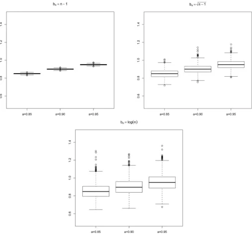
Figure 1 shows three boxplots obtained from estimates ofa∈ {0.85,0.9, 0.95} for various sequences (bn)n≥1 based on 1000 simulated samples of

size n = 50. Here, the underlying renewal process is generated using independent inter-arrival times that follow a Weibull distribution with shape parameter 2 and scale parameter 10. These boxplots show that the convergence rate of ˆanheavily depends onbn. This is consistent with

the fact that in Section 2, we showed that for bn =n−1,√n or logn,

the convergence rate of ˆan is proportional ton3/2,nor

√

n, respectively.

Figure 1: Comparison of boxplots of 1000 estimates of a ∈

{0.85,0.9,0.95}obtained from samples of size 50 forbn=n−1,

√

n−1 and logn.

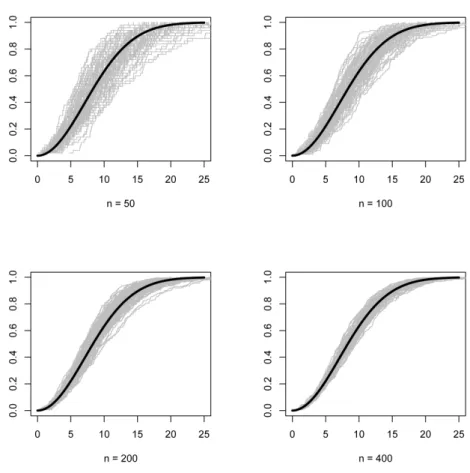
The estimator ˆFn of F is based on the empirical distribution

func-tion obtained from the firstnobservations of the pseudo renewal process

( ˜Yn)n≥1 defined by ˜Yn = ˆa−bnXn. Figure 2 illustrates the uniform

con-sistency result obtained in Proposition 2.4. The cumulative distribution function F (black solid line) is compared with 100 estimates ˆFn (grey

solid lines) forn∈ {50,100,200,400}.

Figure 2: 100 estimates ˆFn (grey solid lines) and the trueF (black solid

line) for various values of n.

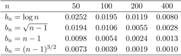
To better illustrate the convergence of ˆFn towards F, we now

cal-culate the empirical mean of N = 1000 Mean Integrated Square Error (MISE) values. For one sample, the MISE equals

1 n

n

∑

i=1

( ˆ Fn

( ˜ Y(i)

)

−F (

˜ Y(i)

))2

= 1 n

n

∑

i=1

(

i/n−F (

˜ Y(i)

))2

,

where ˜Yi = ˆa−nbiXi for 1≤i≤nand ˜Y(i) is the i−th order statistic. F

is the Weibull cdf with scale parameter 10 and shape parameter 2, and a= 2.

n 50 100 200 400

bn= logn 0.0252 0.0195 0.0119 0.0080

bn=

√

n−1 0.0194 0.0106 0.0055 0.0028 bn=n−1 0.0098 0.0054 0.0024 0.0013

bn= (n−1)3/2 0.0073 0.0039 0.0019 0.0010

Table 1: Mean of N = 1000 MISE values

3.2 On the choice of the bn’s

We have assumed that the sequence (bn)n≥1 was known. A natural

question hence is: how can we check the validity of the sequence (bn)n≥1?

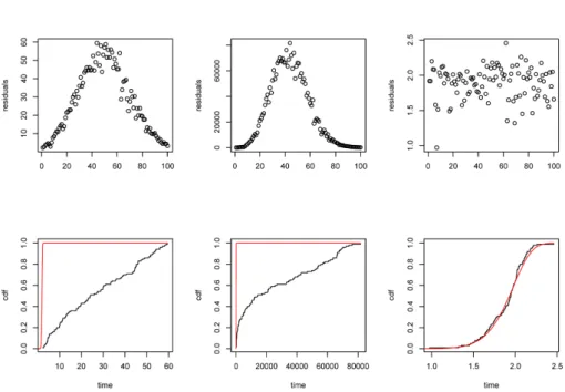
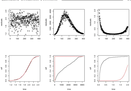
We here propose a residual analysis, based on the fact that, in case of a correct choice forbn and of a ”good” estimate ˆaofa, the residualsk7→

ˆ a−bk_X

k should be nearly i.i.d.. Such residuals and the corresponding

estimated cdf ˆFn are plotted for different situations in Figures 3 and 4,

withbn =nθ0. Such figures clearly illustrate the consequences of a bad

choice for bn.

Looking at the residuals can hence help to chose between several possible choices for bn (between bn = n,

√

n or n3/2 in the previous examples). When the possible choices forbn are unknown, another

ap-proach is required.

In case bn = g(n;θ), where g is a known link function indexed by

θ∈Θ∈Rp, we can estimateθin the following way. Forn≥1, we have: Zn= logXn=g(n;θ)β+µ+en,

where β = loga and µ =E[logY1]. Hence we can estimate µ,β and θ

by minimizing the cost functioncn defined by

cn(µ, β, θ) = n

∑

k=1

(Zk−βg(k;θ)−µ)2.

Figure 3: n = 100, a = 0.98, θ0 = 1.5, columns 1 to 3 correspond to

bn = n, bn =

√

n and bn = n3/2 (true) respectively. At the top are

residuals k 7→ ˆa−bk_X

k while at the bottom are both the estimated cdf

of the renewal process (dotted) and the true cdf (solid).

It is easy to see that both optimal parameters µn(θ) and βn(θ) can be

expressed as functions of θ, with:

µn(θ) =

(∑n_k=1g(k;θ)) (∑n_k=1ykg(k;θ))−(

∑n k=1yk)

(∑n

k=1g2(k;θ)

) (∑n_k=1g(k;θ))2−n(∑n_k=1g2_(k;θ)) ,

(7) βn(θ) =

(∑n_k=1g(k;θ)) (∑n_k=1yk)−n(

∑n

k=1ykg(k;θ))

(∑n_k=1g(k;θ))2−n(∑n_k=1g2_(k;θ)) . (8)

Plugging these two functions intocn(µ, β, θ), we obtain a new cost

func-tion Cn which only depends on θ:

Cn(θ) = n

∑

k=1

(Zk−βn(θ)g(k;θ)−µn(θ))2.

We next minimize Cn(θ) with respect to θ, which provides an estimate

ˆ

θn forθ, and hence an estimate forbn’s (ˆbn=g(n; ˆθn)).

Figure 4: n = 400, a = 0.95, θ0 = 1, columns 1 to 3 correspond to

bn = n (true), bn = √n and bn = n3/2 respectively. At the top are

residuals k 7→ ˆa−bk_X

k while at the bottom are both the estimated cdf

of the renewal process (dotted) and the true cdf (plain).

This procedure is illustrated in Figures 5 and 6 for g(k;θ) = kθ, which show its efficiency.

3.3 Aircraft data

We end this session with the study of a real data set of sizen= 29. This data set contains successive times to failure (operating hours) of an air-conditioning equipment of a Boeing 720 aircraft and it is taken from data corresponding to 13 different aircraft. These data were studied in [21] and are available in [18].

Figure 7 shows the successive failure times (operating hours).

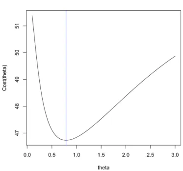
Optimizing the criterion θ 7→ Cn(θ) for bn = (n−1)θ, we obtain

ˆ

θ= 0.788, see Fig. 8.

Table 2 summarizes the results obtained for the estimation of pa-rameter a for various bn’s. The estimate ˆa of a is given with a 95%

Figure 5: n= 100, a= 0.98, θ0 = 1.5,θ 7→ Cn(θ) is the plain curve, θ0

and ˆθnare superimposed vertical lines.

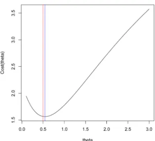
Figure 6: n= 100, a= 0.90, θ0 = 0.5,θ 7→ Cn(θ) is the plain curve, θ0

is the vertical plain line, ˆθn is the vertical dotted line.

Figure 7: Successive failure times of the air-conditioning equipment.

asymptotic confidence interval [ˆamin,aˆmax] which is computed via

Propo-sition 2.3.

bn (n−1)0.788 logn √n−1 n−1 (n−1)3/2

ˆ

a 0.900 0.620 0.740 0.952 0.992 95% CI fora [0.798,1.003] [0.275,0.966] [0.489,0.991] [0.901,1.003] [0.982,1.001]

Table 2: Estimates ofaand various bn’s for the aircraft data.

It is interesting to note that, whatever the choice for bn, the

esti-mate ofabelongs to (0,1). This implies that the times between succes-sive failures are stochastically non increasing. Note also that if we test H0: a= 1 by rejecting the hypothesisH0whenever the 95% Confidence

Interval (CI) for a does not contain 1, then we do not reject H0 when

bn = (n−1)θ with θ= 0.788, 1 or 1.5 while this hypothesis is rejected

whenbn is lognor

√

n−1 (see Tab. 2). It however is highly likely that a <1. Finally, Fig. 9 shows that the estimates of the cdfF also are sen-sitive to the choice of bn: the further bn is from the optimal sequence,

the further the cdf estimates are from the empirical cdf obtained for bn= (n−1)0.788.

4

Application to reliability

A repairable system is now considered, with instantaneous repairs at failure times and successive life-times modeled by an EGP. Once the process has been statistically estimated, it may be used for prediction purposes and/or optimization of replacement policies. As for prediction

Figure 8: θ7→ Cn(θ) for the aircraft data.

purpose, a typical quantity of interest is the mean number of failures on some time interval [0, t]. In case of non increasing lifetimes (a ≤ 1), a replacement policy is next studied, where the system is renewed as soon as a lifetime is observed to be too short. We begin with some preliminary results.

4.1 Preliminary results

Lemma 4.1. Setting T_∞ = lim

n→+∞Tn, we have the following

di-chotomy:

1. If ∑+_i=1∞abi _<+∞_{, then} E_(T

∞)<+∞ (and T∞<+∞ a.s.).

2. If ∑+_i=1∞abi _{= +}∞_{, then T}

∞= +∞ a.s. (and E(T∞) = +∞). Proof. In case a≥1 (which implies ∑+_i=1∞abi _{= +}∞_{), we clearly have:}

Tn ≥ Sn, where Sn =

∑n

j=1Yj. As S∞ = +∞ a.s. (renewal case), we

getT_∞= +∞ a.s..

Figure 9: Empirical cumulative distribution function for the aircraft data.

Let us now assume a∈ (0,1). If ∑_i+₌₁∞abi _{< +}∞_{, we easily derive}

the first point, due to

E(Tn) = n

∑

i=1

E(Xi) =E(Y1)

n

∑

i=1

abi_{. (9)}

As for the second point, let cn =

∑n

i=1abi. Ascn ≥nabn, we have

a2bn_/c2

n≤1/n2 and

∑+∞

n=1a

2bn c2

n <+∞. We derive that

+∞

∑

n=1

Var (Xn)

c2

n

=Var (Y1) +∞

∑

n=1

a2bn

c2

n

<+∞

and in case ∑+_i=1∞abi _{= +}∞_{, Theorem 6.7 from [20] implies that:}

Tn−E(Tn)

cn

= Tn cn −E

(Y1)→0 a.s.

so that T_∞= +∞ a.s..

Remark 4.1. Such results extend similar results from [15] provided in the special case where bi=i−1.

We now look at an example.

Example 4.1. Letbn =nα(log (n))β withα ≥0 and β ≥0, and let

a ∈ (0,1). Then ∑_i+₌₁∞abi _{= +}∞ _{if and only if α = 0 and one of the}

following conditions is fulfilled:

• β <1,

• β = 1 anda≥1/e.

Proof. In case α >0, we have 0≤abn _=anα(logn)β ≤_anα _{for alln}≥_3.

If α ≥ 1, then 0 ≤ abn ≤ _anα ≤ _an_{, from which we derive that}

∑+∞

i=1abi <+∞.

If 0< α <1, we have: a(n+1)α

anα = 1 +αlog (a)n

α−1_+o(_nα−1)

from where we derive that

lim

n→+∞n

(

a(n+1)α anα −1

)

= lim

n→+∞αlog (a)n

α _{=−∞<−1.}

This implies that∑+_n=1∞anα <+∞using Raabe’s rule, and hence∑+_i=1∞abi

<+∞.

In case (α, β) = (0,1), we haveabn _=nlog(a)_{, so that}∑+∞

i=1 abi <+∞

if and only if a <1/e.

For α = 0 and β ̸= 1, the series∑+_i=1∞abi _{has the same behavior as}

∫+∞ 1 a

(log(u))β_{du, with}

lim

u→+∞u

θ_a(log(u))β _{= lim}

u→+∞e

((log(u))β−1log(a)+θ)log(u)

= {

0 if β >1, +∞ ifβ <1,

for all θ > 0. We deduce that ∑+_i=1∞abi _{< +}∞ _{if and only if β > 1,}

which completes this proof.

4.2 Mean number of failures

In order to get a ”pseudo-renewal” equation for the ”pseudo-renewal” function associated to the EGP, we here envision the case where the first interarrival timeX1of the EGP is distributed asXk=abkYk, withk≥1.

This means that at time T0 = 0, the system has already been repaired

k−1 times. The successive interarrival times then are distributed as Xk,Xk+1, . . . This situation is denoted by Φ0 =k.

Fork≥1, we setPk to be the conditional probability measure given

that Φ0 =k, withk≥1 and Ek the associated conditional expectation.

In case k= 1, we have: P=P1 and E= E1. For any intervalI ⊂R+,

we also set N(I) to be the number of failures (or arrivals of the EGP) on I, with

N(I) =

+∞

∑

n=1

1_{Tn∈I}

In caseI = [0, t], we simply set: N(t) =N([0, t]). Given that Φ0 =k, the ”pseudo-renewal” function is

nk(t) =Ek(N(t)) =

+∞

∑

n=1

Pk(Tn≤t)

andnk(t) stands for the mean number of failures on [0, t]. In casek= 1,

we set n(t) =n1(t).

A necessary condition fornk(t) to be finite for allt≥0 isT∞= +∞

a.s. (see [6] in the more general set up of Markov renewal functions), which here writes ∑+_i=1∞abi _{= +}∞_{, see Lemma 4.1. We next provide a}

sufficient condition.

Proposition 4.1. AssumeE(Y1)<+∞and lim

n→+∞na

bn _> 1

E(Y1) (and hence ∑+_i=1∞abi _{= +}∞_{). Then n}

k(t)<+∞ for allt≥0 and all k≥1. Proof. In casea≥1, we have:

nk(t)≤n1(t) =n(t)≤U(t)<+∞,

whereU(t) stands for the renewal function associated to the underlying renewal process.

In case a∈(0,1), let t >0 and k≥1 be fixed. Due to the Markov inequality, we have:

nk(t) =

+∞

∑

n=1

Pk

(

e−Tn ≥_e−t)≤_et

+∞

∑

n=1

un,k

with

un,k=Ek

(

e−Tn)₌ k+_∏n−1

i=k

E(e−abiY1 ) and

lim

n→+∞n

( un+1,k

un,k −

1 )

=− lim

n→+∞na

bk+n×E

(

1−e−abk+nY1 abk+n

)

As 1−e−abk+n Y1

abk+n converges to Y1 when n → +∞ and is bounded by Y1,

we derive by Lebesgues’s theorem that:

lim

n→+∞n

( un+1,k

un,k −

1 )

=− lim

n→+∞na

bn×E_(Y

1)<−1

by assumption. We conclude with Raabe’s rule.

Example 4.2. For bn= (log (n))β withβ ≥0 and a∈(0,1), we get

that nk(t) is finite for all t ≥ 0 and all k ≥ 1 as soon as one of the

following condition is fulfilled:

• β <1,

• β = 1 anda > 1_e,

• β = 1,a= 1_e, and E(Y1)>1.

Such results show that, contrary to classical geometric processes (see [5] and the introduction), it is possible to model decreasing successive lifetimes with extended geometric processes and get a finite expected number of counts at an arbitrary time.

Proposition 4.2. Assume that lim

n→+∞na

bn _> 1

E(Y1). The function nk fulfills the following pseudo-renewal equation:

nk=Fk+fk∗nk+1 (10)

for all k ≥ 1, where Fk (resp. fk) stands for the cumulative (resp.

probability) distribution function of Xk.

Proof. Using classical arguments ([6] e.g.), we have:

nk(t) =Ek

(

N(t)1_{X1≤t})

=Ek

(

Ek(N(t)|X1)1_{X1≤t} ) =Ek

(

Ek(N(]0, X1])|X1)1_{X1≤t} )

+Ek

(

Ek(N(]X1, t])|X1)1_{X1≤t} ) =Fk(t) +

∫

[0,t]

nk+1(t−u)fk(u) du,

which may be written as (10).

Remark 4.2. Setting ΦTn = k in case Xn+1 is distributed asa bk_Y

k

(with k≥n+ 1) and Φt= ΦTn forTn≤t < Tn+1, the process (Φt)t≥0

then appears as a semi-Markov process with semi-Markov kernel pro-vided by

q(i, j, dx) =1_{j=i+1}dFi(x).

Equation (10) then is the Markov renewal equation satisfied by the cor-responding Markov renewal function.

We now provide practical tools for the numerical assessment of the pseudo (Markov) renewal function nk(t).

Corollary 4.1. Assume a≥1. Setting un(t) =P(Tn≤t),

for all n≥1, we have:

0≤ n(t)− ∑N

n=1un(t)

n(t) ≤uN(t), (11) for all N ≥1. Also,(un(t))_n≥1 may be computed recursively using

u1(t) =F(t)

un+1(t) = (fn+1∗un) (t) =

1 abn+1

∫ t

0

un(u)f

( t−u abn+1

)

du (12)

for all n≥1, whereF (resp. f) stands for the cumulative (resp. proba-bility) distribution function of Y1.

Proof. We may write:

n(t) =

N

∑

n=1

un(t) +εN(t)

where

εN(t) =

+∞

∑

m=1

P(Tm+N ≤t).

Using similar arguments as [11], we have

{Tm+N ≤t}={TN + (Tm+N−TN)≤t} ⊂ {TN ≤t}∩{Tm+N −TN ≤t}

whereTN and Tm+N −TN are independent. We derive:

εN(t)≤P(TN ≤t)

+∞

∑

m=1

PN(Tm≤t) =uN(t)nN(t)≤uN(t)n(t),

which implies (11). The remainder of the proof is straightforward.

Remark 4.3. This result allows to numerically assess the pseudo renewal function n(t) up to a given precisionε >0 by recursively com-putingun(t) untilun(t) is smaller thanε. Note however that theui(t)’s

are computed using discrete convolutions in (12), which induces numer-ical errors. Such errors might be quantified using similar methods as in [19].

In case a < 1, the previous result is not valid because nN(t) ≥

n(t). In that case, Monte-Carlo simulations may be used to compute the pseudo-renewal function. A lower boundnc_{(t) may also be provided,}

which converges ton(t) whencgoes to zero. This bound is constructed via the following lemma.

Lemma 4.2. For c >0 and t≥0, let

τc= inf (n≥1 :Xn< c) (13)

and

nc(t) =E (_τc₋₁

∑

n=1

1_{Tn≤t}

)

(0 in case of an empty sum). Then nc(t)≤n(t) and

lim

c→0+n

c_{(t) =n(t).}

Proof. Using the fact that τc _{increases to infinity when c decreases}

to 0+, the result is a direct consequence of the monotone convergence theorem.

The following lemma provides tools for the numerical assessment of nc(t), which do not requirea≥1.

Lemma 4.3. Setting

uc_n(t) =P(Tn≤t, X1≥c, . . . , Xn≥c)

for all n≥1, we have:

nc(t) =

⌊t c⌋

∑

n=1

uc_n(t), (14)

where ⌊...⌋ stands for the floor function. Also,(uc_n(t))_n≥1 may be com-puted recursively using

uc₁(t) = (F(t)−F(c))+ uc_n+1(t) = 1

abn+1

∫ (t−c)+

0

uc_n(u)f (

t−u abn+1

)

du (15)

for all n≥1.

Proof. We have:

nc(t) =

+∞

∑

n=1

P(Tn≤t, n < τc) =

+∞

∑

n=1

P(Tn≤t, X1 ≥c, . . . , Xn≥c).

Noting that X1 ≥c, . . . , Xn ≥ c implies Tn ≥ nc, the summation may

be restricted ton≤⌊_ct⌋, which provides (14). Equation (15) is a direct consequence of

uc_n+1(t) =E(E(1_{Tn≤t−Xn+1}1{X1≥c,...,Xn≥c}|Xn+1

)

1_{Xn+1≥c} ) =E(uc_n(t−Xn+1)1_{Xn+1≥c}

)

= 1

abn+1 ∫ t

c

uc_n(t−u)f

( _u

abn+1 )

du for all t≥c.

4.3 A replacement policy

We here consider the case wherea <1 and the following renewal policy is considered: as soon as a lifetimeXi is observed to be shorter than the

predefined threshold s (s > 0), the system is instantaneously replaced at some cost cR. Between replacements, the cost of an instantaneous

repair which follows a failure is denoted by cF, with cR ≥ cF. We set

c(s) to be the asymptotic unitary cost per time unit time.

The next proposition uses classical results from renewal theory to derive the existence of c(s), and an expression for it.

Proposition 4.3. Assume a ∈ (0,1). Setting C([0, t]) to be the cumulated cost on [0, t], the asymptotic cost per unit time

c(s) = lim

t→+∞

C([0, t])

t a.s. (16)

exists and is provided by

c(s) = cR+cFE(τ

s₋₁₎

E(Tτs) , (17)

where τs is defined asτc, see(13). Furthermore,

E(τs−1) =

+∞

∑

k=1

vs_k

E(Tτs) =E(Y₁)

( 1 +

+∞

∑

k=1

abk+1 _vs

k

)

with

v_ks =

k

∏

i=1

¯ F

( _s abi

)

(18)

for all k≥1 and F¯ = 1−F.

Proof. The evolution of the maintained system may be described by a regenerative process, with cycles delimited by the replacement of the

system and generic length Tτs. Moreover

E(Tτs) =

+∞

∑

k=2

E(Tk

(

1_{τs_≥k}−1_{τs_≥k+1}

))

+E(T11_{τs_=1}

)

=

+∞

∑

k=3

E((Tk−Tk−1)1_{τs_≥k}

)

+E(T21_{τs_≥2}

)

+E(X11_{τs_=1}

)

=

+∞

∑

k=1

ws_k,

with

ws_k=E(Xk1_{τs_≥k}

) =abkE_(Y

k)P(X1 ≥s, ..., Xk−1 ≥s)

=abkE_(Y

1) vks−1,

for all k≥2 andws₁=E(Y1).

Now, as

lim

k→+∞

ws_k+1

ws_k = limk→+∞a

bk+1−bk_F¯

( _s abk

) = 0,

the series with generic term ws_k is convergent andE(Tτs)<+∞.

We derive the existence ofc(s) and formula (17) (see [1] e.g.), noting that the mean cost on a generic cycle is cR+cFE(τs−1).

The quantity E(τs) may finally be computed via:

E(τs) =

+∞

∑

i=1

P(τs≥i) = 1 +

+∞

∑

i=2

P(X1 ≥s, ..., Xi−1≥s) = 1 + +∞

∑

i=2

v_is₋₁.

We next provide tools for the numerical assessment of c(s).

Proposition 4.4. Assume a∈(0,1). We have the following bounds for c(s) :

mN_c (s)≤c(s)≤M_cN(s), where

mN_c (s) = cR+cF S

N

1 (s)

E(Y1)

(

1 +S₂N(s) +abN+2 _vs

N+1/F

(

s abN+2

)),

M_cN(s) =

cR+cF

(

S₁N(s) +vs_N+1/F (

s abN+2

))

E(Y1)

( 1 +SN

2 (s)

) ,

and

S₁N(s) =

N

∑

k=1

vs_k,

S₂N(s) =

N

∑

k=1

abk+1_vs

k

(with v_ks defined by(18)). Moreover we have

c(s)−m

N

c (s) +McN(s)

2

≤∆cN_max(s) := M

N

c (s)−mNc (s)

2 .

Proof. We have

1 +

N

∑

k=1

abk+1 _vs

k≤

E(Tτs)

E(Y1) ≤

1 +

N

∑

k=1

abk+1 _vs

k+

+∞

∑

k=N+1

abk+1 _vs

k,

with

+∞

∑

k=N+1

abk+1 _vs

k≤abN+2

+∞

∑

k=N+1

v_ks,

and

+∞

∑

k=N+1

v_ks≤vs_N+1×

+∞

∑

k=N+1

( ¯ F

( _s

abN+2

))k−N−1

= v s N+1 F ( s abN+2

). We derive

E(Y1)

(

1 +S₂N(s))≤E(Tτs)≤E(Y₁)



1 +S₂N(s) +a

bN+2_vs

N+1

F (

s abN+2

)  .

A similar method is used for bounding E(τs_{), which provides the}

result.

This proposition allows to numerically assess the cost function c(s) up to a given precision ε by recursively computing S₁N(s) and S₂N(s) until ∆cN_max(s) is smaller than ε.

4.4 Numerical experiments

4.4.1 Computation of the pseudo-renewal function

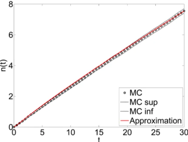
We first consider the case where a ≥ 1. The random variable Y1 is

Gamma distributed with shape parameter 1.2 and scale parameter 2.5 (which providesE(Y1) = 3,Var (Y1) = 7.5). This distribution is denoted

by Γ (1.2,2.5). We also take bn = n0.3 and a = 1.2. The

approxima-tion of the pseudo-renewal funcapproxima-tion n(t) provided by Corollary 4.1 is plotted against t in Figure 10 for N = 20. The maximal relative error provided by the approximation is about 4.2×10−6. We also plot n(t) computed by Monte-Carlo simulations and the 95% confidence band for 103 trajectories in the same figure. The results are quite similar.

Figure 10: n(t) with respect totby Monte-Carlo simulations (MC) and by the approximation provided by Corollary 4.1.

We next consider the case where a < 1 (and lim

n→+∞na

bn _> 1

E(Y1)): the random variable Y1 follows Γ (2.5,1) with E(Y1) =Var (Y1) = 2.5,

bn= (logn)0.7anda= 0.8. The lower boundnc(t) forn(t) is computed

via the results of Lemma 4.3 for different values ofc (c= 0.05, c= 0.1, c= 0.25, c= 0.5). The results are displayed in Figure 11. As expected (see Lemma 4.2),nc(t) is stabilizing whencgoes to zero and the values for c = 0.05 and c = 0.1 are nearly super-imposed. We also plot n(t) computed by Monte-Carlo simulations and the 95% confidence band for

103 trajectories in Figure 12, as well as nc(t) for c= 0.05. We observe thatnc(t) is a good approximation ofn(t) for small c.

Figure 11: nc(t) with respect tot for different values ofc.

Figure 12: n(t) by Monte-Carlo simulations and nc(t) for c= 0.05.

4.4.2 The replacement policy

The random variable Y1 follows Γ (2.5,1) with E(Y1) = Var (Y1) = 2.5,

bn= (logn)0.7,a= 0.8,cR= 1 and cF = 0.5.

For N = 100, the maximal absolute error ∆cN_max(s) decreases very quickly assincreases (∆cN_max(0.4)≃8×10−5, ∆cN_max(0.7)≃3×10−12, beyond the machine precision for s ≥ 0.9). The cost function c(s) is plotted against sin Figure 13. The cost function reaches its minimum atsopt≃1.70, with min

s>0 c(s) =c

(

sopt)≃0.17.

Figure 13: c(s) with respect tos.

5

Concluding Remarks and Prospects

Contrary to renewal processes, geometric processes proposed by [17] and their present extension both allow successive inter-arrival times to be (stochastically) increasing or decreasing. From a modelling point of view, the extended version has however been seen to be more flexible. Also, in an applied context, the expected number of arrivals of the un-derlying counting process on some finite time interval is expected to be finite at any time. This had previously been seen by [5] to be incom-patible with a decreasing geometric process. In contrast, GP’s extended geometric processes do not suffer from this drawback. Extended geo-metric processes may hence be a simple alternative to the virtual age models proposed by [9] and [13] for the modeling of imperfect mainte-nance actions e.g..

From the estimation point of view, we saw that the convergence rate of the estimator of the Euclidean parameter astrongly depends on

the sequence (bn)n≥1. A miss-specification of the sequence (bn)n≥1 will

naturally lead to biased estimates. To make the model more flexible, we hence considered a parametrized version of the sequence (bn)n≥1 by

settingbn=g(n, θ), whereθis an additional Euclidean parameter. Some

procedure has been provided for its estimation.

Note the lack of a central limit theorem for the estimator ˆF of the underlying cumulative distribution function F. Indeed, standard meth-ods cannot be used here, because of the deterministic nature of the bn’s. This problem hence requires some more investigation along with

the study of the properties of the estimator of θ for parametrized se-quences bn=g(n;θ). Such a result would however be useful for testing

the hypothesis that the underlying cumulative distribution function F belongs to some parametric family. Another possible issue would be to include covariates in this model in order to describe (e.g.) the effect of the environment on the monotonicity of the EGP.

In case a < 1, a lower bound has been provided for the pseudo-renewal function, which is easy to compute using Lemma 4.3. However, we haven’t been able to provide a computable upper bound, although it is necessary for the numerical assessment of the results precision. In-deed, the usual tools such as those used in case a≥1 are inappropriate here, and new tools should be developed. As for the replacement policy, because of the random character of the successive lifetimes, an alternate policy based on a predefined numberm of consecutive lifetimes under a thresholds, might be better adapted than the present policy, based on a replacement at the first observation of a single lifetime below s.

References

[1] Asmussen, S. (2003), Applied probability and queues. Applications of Mathematics,51, Second ed., New York: Springer-Verlag. [2] Barlow, R. E. and Proschan, F. (1996), Mathematical theory of

re-liability. Classics in Applied Mathematics, vol. 17, fifth ed., Society for Industrial and Applied Mathematics (SIAM), Philadelphia, PA, 1965, With contributions by Larry C. Hunter.

[3] Bai, Z. D., Cheng, P. E., and Zhang, C. H. (1997), An extension of Hardy-Littlewood strong law. Statistica Sinica, 923–928.

[4] Bai, Z. D., Cheng, P. E. (2000), Marcinkiewicz strong laws for linear statistics. Statistics & Probability Letters,46, 105–112.

[5] Braun, W. J., Li, W., Zhao, Y. Q. (2005), Properties of the geomet-ric and related processes. Naval Research Logistics,52, 607–616. [6] C¸ inlar, E. (1975), Introduction to Stochastic Processes. Englewood

Cliffs, NJ: Prentice-Hall.

[7] Cook, R. J. and Lawless, J. F. (2007), The Statistical Analysis of Recurrent Events. Springer.

[8] Cuzick, J. (1995), A strong law for large for weighted sums of I.I.D. random variables. Journal of Theoretical Probability, 8(3), 625– 641.

[9] Doyen, L. and Gaudoin, O. (2004), Classes of imperfect repair mod-els based on reduction of failure intensity or virtual age. Reliability Engineering & System Safety 84(1), 45–56.

[10] Finkelstein, M. (2010), A note on converging geometric-type pro-cesses. Journal of Applied Probability,47, 601–607.

[11] Feller, W. (1968), An introduction to probability theory and its applications. Vol. 1. New York: John Wiley & Sons Inc.

[12] Feller, W. (1971), An introduction to probability theory and its applications. Vol. 2. New York: John Wiley & Sons Inc.

[13] Kijima, M. (2002), Stochastic models in reliability and mainte-nance. Osaki, Shunji ed., ch. Generalized Renewal Processes and General Repair Models, 145–164, Berlin: Springer.

[14] Lam, Y. (1992), Nonparametric inference for geometric processes. Communications in Statistics-Theory and Methods,21, 2083–2105. [15] Lam, Y., Zheng, Y. H., and Zhang, Y. L. (2003), Some limit theo-rems in geometric processes. Acta Mathematicae Applicatae Sinica,

19, 1–12.

[16] Lam, Y., Zhu, L. X., Chan, S. K. and Liu, Q. (2004), Analysis of data from a series of events by a geometric process model. Acta Mathematicae Applicatae Sinica,20, 263–282.

[17] Lam, Y. (2007), The Geometric Process and its Applications. World Scientific.

[18] Lindsey, J. K. (2004), Statistical Analysis of Stochastic Processes in Time, Cambridge University Press, Cambridge.

[19] Mercier, S. (2008), Numerical bounds for semi-markovian quanti-ties and application to reliability. Methodology and Computing in Applied Probability,10(2), 179–198.

[20] Petrov, V. V. (1995), Limit Theorems of Probability Theory: Sequences of Independent Random Variables. Oxford University Press.

[21] Proschan, F. (1963), Theoretical explanation of observed decreasing failure rate. Technometrics,5, 375–383.

[22] Van der Vaart, A. W. (1998), Asymptotic Statistics. Cambridge: Cambridge University Press.