Autumn 2014
A two-stage model for cell formation problem considering the
inter-cellular movements by automated guided vehicles
Saeed Dehnavi-Arani
1*, Mohammad Saidi Mehrabad
Department of industrial engineering, Iran University of Science and Technology, Iran, Tehran [email protected], [email protected]
Abstract
This paper addresses to the Cell Formation Problem (CFP) in which Automated Guided Vehicles (AGVs) have been employed to transfer the jobs which may need to visit one or more cells. Because of added constraints to problem such as AGVs’ conflict and excessive cessation on one place, it is possible that AGVs select the different paths from one cell to another over the time. This means that the times and costs between cells are dynamic. The proposed model consists of 2 stages that stage (1) is related to a basic CFP, with a set of machine cells and their corresponding job families, while stage (2) is related to finding AGVs’ routing, to determine the dynamic costs. For solving this problem, a two-stage heuristic algorithm based on an exact method has been proposed. A computational experiment has been solved to show efficiency of proposed heuristic.
Keywords: Cell formation problem, Routing problem, Automated guided vehicle, Two-stage model, Two-Two-stage heuristic
1. Introduction and review
Cellular Manufacturing System (CMS) is the application of the principles of Group Technology(GT) in manufacturing system (Ghezavati and Saidi mehrabad, 2009). CMS is a production system in which jobs with the same manufacturing process are placed in one group, called job family. Each job family is assigned to one cell. In this way, several advantages are obtained such as reduction in setup time, throughput time, work-in-process inventories, and material handling cost, better quality and production control and enhancement in flexibility. CMS also provides a production infrastructure to implement modern manufacturing technologies such as computer integrated manufacturing, flexible manufacturing system and just-in-time (Pasupuleti, 2012).There are several
*
Corresponding Author
issues about designing and controlling the CMS such as layout of CMS, Cell Formation Problem (CFP), production planning in CMS, scheduling and sequencing of the jobs in CMS, etc. ( Tavakkoli Moghaddam, Gholipour Kanani and Cheraghalizadeh, 2008)
CFP is one of the most important issues of CMS and if this problem cannot be implemented effectively, advantages of CMS won’t attain for that company or organization. In a basic CFP, each job family and each machine is assigned to one of manufacturing cells with considering the defined constraints so that the objective function can be optimized. In other words, the machine groups and job families assigned to each cell are determined in a basic CFP.
In the initial papers, many authors have assumed that each job can be assigned to only one single cell and no jobs need the other cells. Whereas in the real-life CMS environment, it could be some exceptional jobs which need to visit machines in the other manufacturing cells. This fact provides the contexts for subsequent researchers to consider inter-cellular jobs movements in theirs researches. As a result, the CFP with considering the times between cells at either objective function or constraints acquired more popularity since 1980. After 1980, minimizing the inter-cellular movements for jobs has been the objective function of most models in CFP area.
As an example, James, Brown and Keeling (2007), presented a hybrid grouping genetic algorithm for abi-objective cell formation problem with one objective of minimizing the inter-cellular movements while other two maximize machine utilization. They tested the proposed algorithm on the several test problems and concluded that it outperforms the standard grouping genetic by both finding the better quality solutions and reducing the variability between solutions. Aljaber, Baek and Chen (1997), proposed a new machine-component clustering heuristic based on tabu search optimization method. The objective function was to minimize the inter-cells movements to minimize, indirectly, the distances between machines of the same machine group and parts of the same part family. They conclude that although the proposed algorithm requires more CPU time rather than other algorithms, but the quality of solutions is enhanced. Also Gravel, Luntala and Price (1998), solved a multi-objective cell formation problem so that the products have multiple routings. They considered two objectives including minimizing the volume of inter-cellular movements and balancing the load among machines in a cell. For solving this model, they use the weighted sum and epsilon constraint method to obtain the set of non-dominant solutions. Lozano et al. (2001), introduced a cell formation problem in which each part has sequence of operations to be placed on each machine. The considered objective function is minimization of both intra-cellular and inter-cellular movements. This problem was solved by two energy-based neural network approaches and the Potts Mean Field Annealing (PMFA). From performance point of view, PMFA has the best performance than two other approaches. Liang and Zolfaghari (1999), considered a comprehensive grouping problem where both the process times and machine capacities are taken into account in the analysis. They presented a new neural network approach and tested it on 28 test problems existing in the literature. The efficiency of this approach is seen in all of the test problems. An Adaptive Genetic Algorithm (AGA) has been proposed in Mak, Wong and Wang (2000) for manufacturing CFP. The difference between proposed algorithm and traditional genetic algorithms is that AGA uses an adaptive scheme to enable crossover and mutation rates to be changed during search process. Finally, efficiency of AGA has been shown especially for large-sized problems. Spiliopoulos and Sofianopoulou (2008), proposed an efficient ant colony optimization system where the objective function was to minimize the inter-cellular
movements. Moreover, the inter-cellular costs as the sum of products that they need to visit two machines located at two distinct cells in two successive steps was defined. The first Particle Swarm Optimization (PSO) could be observed in Andres and Lozano (2006) for CFP. They compared PSO with published exact results to assess the proposed algorithm. The results showed that the PSO algorithm was able to find the optimal solution on all of instances. Safaei et al. (2008), presented a CFP with a dynamic product mix and demand rate in multi-period planning horizon. They developed a fuzzy programming approach by assuming that inter-cellular and intra-cellular movement costs per batch are assumed predefined. Tavakkoli Moghaddam et al. (2010), solved a multi objective CFP with considering the machine utilization and alternative process routes by scatter search algorithm. The second objective function of their paper is minimizing the cost of inter-cellular movements.
Furthermore, they assumed that inter-cellular material cost for each batch is fixed over the time. In all of the above-mentioned papers and other papers in CFP like (Arkat, Hosseini and Farahani,
(2011), Chung, Wu and Chang, (2011), Elbenani, Ferland and Bellemare, (2012), Guerreo et al. (2002), Jolai et al.,9 2012), Li, Baki and Aneja,(2010), Mahdavi et al.,( 2009), Pilla et al.,(2010), Prabhaharan et al.,( 2004), Solimanpur, Saidi and Mahdavi, (2010) and Wu et al. ( 2004), Wu, Chung and Chan, (2009), Wu, Chung and Chang, (2010)) the movement times from a cell to other cell are assumed to be deterministic and predefined and are considered fix over the time. While in practice, these costs may change
In this paper, we introduced a model for CFP where the movement times between cells change along the time and also the costs between cells are dynamic since costs are proportionate to the time. In each CMS that the automatic material handling systems like AGVs have been employed to transfer the jobs, inter-cellular costs cannot be assumed as constant and predefined values. For example, when AGVs are moving from one cell to another, it would be possible that they select various routes along time so that they don’t crash to other AGVs or it would be possible that an AGV stop of a point on the network because other AGV may be cross its route. In this study the dynamic time in a production environment is considered and can be applicable for every production environment which uses the automatic vehicles in system.
In this article a two stage GAMS-based heuristic algorithm is developed. The algorithm includes two stages so stage 1 performs machine groups and determines the job families and assigns job families to cells while in stage 2, by using the results obtained from stage 1 and AGVs routing, the dynamic costs are found.
2. Problem description
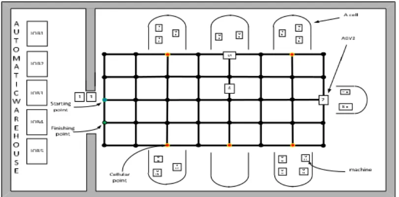
The considered operational system, is a CMS environment, with machines and inter-cell AGVs. A number of jobs in automatic warehouse should be processed on machines. These jobs may need to one or more cells. First the machines should be assigned to the cells for determining jobs required cellular points. Afterwards, AGVs transfer jobs from starting point to their required cellular points through network guide-path and then deliver them to cells. In here, we consider more than one AGV among the cells. Then the cells deliver semi or finished jobs to AGVs. AGVs transfer semi-finished jobs to other cells and finished jobs to ending point (warehouse). A schema of studied problem in this
paper has been shown in figure 1. Generally, the problem is composed of two sub-problems 1) assignment of machines to cells and 2) AGV’s routing. In addition, the following assumptions have been considered in this paper:
All AGVs have unit-job capacity
AGV and machines operate continuously without breakdown.
AGVs loading and unloading times are fixed and are argumented to travel times
AGV that conveys a job can stop only of required cellular points for same job.
A new job cannot be assigned to an occupied AGV.
machines are not identical
AGVs receive jobs from starting point and deliver them to ending point. These two points are
determined on the network.
It is possible that a cell remains without any machine assigned to it.
Figure 1: A scheme of operational system
3. The mathematical model
In this section, the mathematical model of two stages is represented. The sets, parameters and variables related to these two stages are as follows:
3.1. Stage 1
A
The set of all machines in shopC
Set of cellsv
Capacity of machine mv
Capacity of cell c1 if machine is assigned to cell
0 otherwise
mc
m
c
p
3.1. 1. Model 1
1
mc c C
p
m
A
(1)mc m c
m A
p
V
c
C
(2)Constraint (1) ensures that each machine would be assigned to only one cell and constraint (2) prevents violation of the capacity of each cell.
3.2. Stage 2
Besides the sets, parameters and variables defined above, the following are necessary to model the stage 2.
( , ) The set of coordinates of points on the network The set of AGVs
The set of jobs in automatic warehouse The set of available time
1 if point ( , ) is a cellular point for job
0 otherwise
ijs
i j
s
b
1 if cellular point ( , ) precedes cellular point ( ,
) for job
0 otherwise
iji j s
i j
i j
s
z
Of course some equations should be established between two above-defined parameters which are as follows:
ijs iji j s i j ijs i j s
z
z
b
b
( , ),( ,
i j
i j
)
( , ),
I J
s
S
(3)ijs i j s i j s ijs iji j s
b
a
b
a
M
z
( , ),( ,
i j
i j
)
( , ),
I J
s
S
(4)ijs i j s i j s ijs i j ijs
b
a
b
a
M
z
( , ),( ,
i j
i j
)
( , ),
I J
s
S
(5)1 if machine is required for job in cellular point ( , )
0 otherwise
ijms
m
s
i j
r
ijs
a
The sequence of cellular point (i, j) for job sijs
t
Operation time for job s in cellular point (i, j)ijms
t
Operation time for job s on machine m in cellular point (i, j)ij
t
Movement time of intra-cellular AGV for a single loop in cellular point (i, j)( , )
a b
Start point where inter-cellular AGVs receive jobs from automatic warehouse( , )
a b
End point where inter-cellular AGVs delivers jobs from automatic warehouse
Travel time between two points of network ( in this article is considered equal to 1)M A big positive number
1 if AGV which transmit job in time is in point ( , )
0 otherwise
ijkst
k
s
t
i j
x
1 if job is received by AGV in time
0 otherwise
kst
s
k
t
y
s
CT
Completion time of job sT Maximum completion time
3.2.1. Model 2
min
T
(6)s
T
CT
s S (7)0
H
s a b kst
t k K
CT
t x
s S (8)0
H
ijs ijkst
t k K
x
b
( , )
i j
( , ),
I J s
S
(9)0 0
(1
)
H H
iji j s
ijkst i j kst
t k K t k K
t x
t x
M
z
( , ), ( ,
i j
i j
)
( , ),
I J
s
S
1
ijkst k K s S
x
( , )
( , ) ( , ),
(0,
)
i j
I J
a b
t
H
(11)
1 1 1
3 (
1)
ij kst ijk s t ijkst ij k s t
x
x
x
x
( , )
( , ), ,
,
,
i j
I J
k k
K k
k
s s
S
s
s
(12)1 1 1
3 (
1)
i jkst ijk s t ijkst i jk s t
x
x
x
x
( , )
( , ), ,
,
,
i j
I J
k k
K k
k
s s
S
s
s
(13)1
ijkst i I j J
x
k
K s
,
S t
,
(0,
H
)
(14)1 1 1 1 1 1 1 1
1
ijkst i jkst i jkst ij kst ij kst
ijs ijkst
x
x
x
x
x
x
b
( , )
( , ),
,
,
(0,
)
i j
I J s
S
k
K t
H
(15)
kst abkst
y
x
k K s, S t, (0,H) (16)1
kst a b ks t s S s s
y
x
,
,
(0,
)
0
k
K s
S t
H
t
(17)0
1
ks s Sy
k
K
(18)0
1
H
kst
t k K
y
s S (19)1
ijkst s S i I j J
x
k
K t
,
(0,
H
)
(20)(
1) x
ijs t t
ijs ijs
ijkst ijkst
t t
x
t
b
s
( , )
i j
S t
,
( , ),
(0,
I J
H
)
k
K
,
(21)ijs ijms ijms ijs s
m A
t
t
r
b
t
( , )
i j
( , ),s S
I J
(22)
Constraint (1) assures that each machine assigns to only one cell. Constraint (2) controls the machines to be assigned to cells with respect to capacity limitation of cells. Constraints (3-5) determine required cells and their sequence. The objective function (6) minimizes the maximum completion time. Constraint (7) says that maximum completion time is greater than all of completion times for set of jobs. Constraint (8) computes completion time for each job which is equal to time that
a job reaches to ending point ( , ). Constraint (9) states that each cellular point for each job s should be visited by one AGV while other points should not be visited, certainly. This means that the points except the cellular points for job s can be visited or not. Constraint (10) ensures that if cellular point ( , ) precedes cellular point ( , ) for job s thus arrival time of AGV to ( , )is earlier than arrival time to ( , ) for the same job. Constraint (11) indicates that in every time, it can be only one AGV of each point except the start point. In fact, this constraint prevents point conflict of AGVs on the network. Constraints (12) and (13) guarantee that AGVs should had no conflicts on the horizontal and vertical edges of the network. Constraint (14) states that each AGV cannot be located in more than one point simultaneously. Constraint (15) specifies that if AGV has been located in a cellular point ( , ) either it can go into four adjacent points including ( + 1, ), ( −1, ), ( , + 1) and
( , −1) or it can stay there in the next time unit. Furthermore, if it has been located in a non-cellular point ( , ), it can only go into four adjacent points. Constraint (16) ensures that a can be assigned to an AGV only if it has been located in the start point ( , ). Constraint (17) says that a new job can be assigned to an AGV if only a job had been delivered to automatic warehouse by the same AGV at the next unit time. Constraint (18) states that each AGV should receive a job at time 0, surely. Constraints (19) indicates that each job can be assigned to only one AGV and constraint (20) says that each AGV can be only responsible for transferring one job. Constraint (21) states that an AGV waits for
t
ijsunit time (operation unit time for job s in cellular point ( , ) in cellular points required for job s. Constraint (22) computes that for each job at each cell is equal to operation times on machines required for that job at that cell plus a single loop time which is movement time of intra-AGV in one loop.4. Solution method and computational experiment
4.1. Solution method
A two-stage heuristic based on exact method is developed for solving this problem. The first stage solves the assignment of machines to cells while the second stage finds the best routes for AGVs. The steps of heuristic algorithm are as follows:
Step 0: don’t assign any machine to any cell and put the optimal cost equal to positive infinity (ASSsel = and Costopt = +). Put the number of iteration equal to zero (N=0). Go to step 1.
Step 1: assign machines to cells randomly (ASSsel= ASSrandom) so that the sum of assigned capacity of machines to each cell doesn’t exceed the capacity of that cell.
Step 2: solve the model 2 described at section 4.2 with considering ASSsel. In this way, by acquiring the dynamic costs, an optimal objective function (OFopt) would be found. If OFopt is smaller or equal than Costopt, go to step 3, otherwise go to step 4.
Step 3: put Costopt = OFopt and ASSopt = ASSsel. Increase one unit the number of iteration (N=N+1) and if N is smaller than the determined iteration (N < DI) go to step 5, Otherwise go to step 6.
Step 4: replace ASSopt with ASSnew by changing two machines selected randomly (ASSsel = ASSnew). Afterwards, go to step 2.
Step 5: replace ASSopt with ASSnew so that machine including the bigger process time at cell including
the bigger process time should be located at cell including the least process time. In such conditions, if capacity of the cell exceeds its limit, machines with the least process time in the cell should be located at cell. Send out machine with maximum process time. Of course, by caring out this rule, if ASSnew is repeated, another machine at the same cell which has the bigger process time, will selected. Now, put ASSsel = ASSnew and go to step 2.
Step 6: ASSopt and Costopt display optimal assignment and the cost of problem, respectively.
The above heuristic algorithm is not efficient for Medium or large sized problem since the solution time will be increased exponentialy. In the next section, a small sized example and obtained results
will be represented.
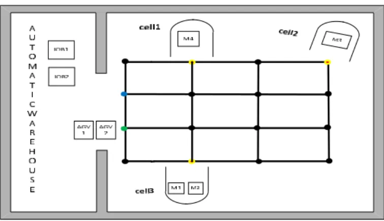
4.2. Illustrative example
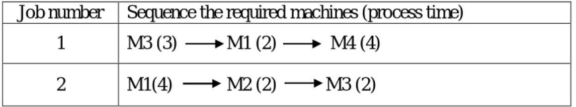
Consider a problem with two inter-cellular AGVs, three cells and four machines is considered. Jobs information including the required machines and processing times have been showed in Table 1. There are sixteen points with coordinates
( , )
i j
i
0,1, 2, 3
andj
0,1, 2, 3
. Furthermore, cells 1, 2 and 3 have been represented with cellular points(1,3)
,(3, 3)
and(1,0)
, respectively. In this example =1 and DI=4. Starting point and end points are(0,1)
and(0, 2)
. The production environment obtained from the first stage has been shown in Figure 2. The steps of proposed heuristic have been represented in Table 2.Table 1: job information including the required machines and processing times
Table 2: The steps of proposed heuristic and to reach to optimal solution
Job number
Sequence the required machines (process time)
1
M3 (3) M1 (2) M4 (4)
2
M1(4) M2 (2) M3 (2)
step
ASS
sel(machine to cell)
OF
optCost
optASS
opt(machine to cell)
0 --- --- +
---1 4 to 1; 3 to 2; 1,2 to 3 24 24 1, 2 to 3; 3 to 2; 4 to 1
2 1,4 to 1; 3 to 2; 2 to 3 22 22 1,4 to 1;3 to 2; 2 to 3
Table 2: continue
step
ASS
sel(machine to cell)
OF
optCost
optASS
opt(machine to cell)
4 1 to 1; 3,4 to 2; 2 to 3 25 22 1,4 to 1;3 to 2; 2 to 3
5* 1 to 1; 4 to 2; 2,3 to 3 21 21 1 to 1; 4 to 2; 2,3 to 3
6 1 to 1; 2,4 to 2; 3 to 3 22 21 1 to 1; 4 to 2; 2,3 to 3
7 1 to 1; 2 to 2; 3,4 to 3 24 21 1 to 1; 4 to 2; 2,3 to 3
8 1 to 1; 2,3 to 2; 4 to 3 25 21 1 to 1; 4 to 2; 2,3 to 3
X*
=
Xis
the optimal stepFigure 2: The production environment obtained from the first stage of heuristic
As it is seen above, the optimal solution for this example is obtained at stage 5. The optimal solution is that machine 1, 2, 3 and 4 should be assigned to cell 1, 3, 3 and 2, respectively. In this state, the optimal cost is equal to 21.
4. Conclusion
A cell formation problem (CFP) where automated guided vehicles (AGVs) transfer the inter-cellular jobs was considered in this article. In such condition, in order to prevent the AGV’s conflict, AGVs would select different routes between two cells over the time. As a result, the inter-cellular costs would be dynamic. In this paper, a two stage mathematical model was represented so that model 1 and model 2 formulate tactical and operational aspects, respectively. To solve this models a two stage heuristic algorithm was proposed. A simple example was solved to be validated both proposed model and algorithm.