Quasi-reflection-based symbiotic organisms search algorithm for solving static optimal power Flow problem

(1)

Sharif University of Technology

Scientia Iranica

Transactions D: Computer Science & Engineering and Electrical Engineering http://scientiairanica.sharif.edu

Quasi-reection-based symbiotic organisms search

algorithm for solving static optimal power ow problem

A. Saha

_{, A.K. Chakraborty, and P. Das}

Department of Electrical Engineering, National Institute of Technology, Agartala, India. Received 1 October 2016; received in revised form 20 February 2017; accepted 18 September 2017

KEYWORDS OPF;

POZ;

Quadratic fuel cost function;

QRSOS; SOS;

Valve-point loading.

Abstract. This paper oers a novel variant to the existing Symbiotic Organisms Search (SOS) algorithm to address the Optimal Power Flow (OPF) problems considering eects of valve-point loading (VE) and prohibited zones (POZ). Problem formulation includes minimization of cost, loss, Voltage Stability Index (VSI), Voltage Deviation (VD), and simultaneous minimization of their combinations. Quadratic cost function, eects of VE, and eects of both VE and POZ have been considered. OPF formulation considering eects of both VE and POZ is not yet available in the literature. Ecacy of SOS in resolving OPF is recognized in the literature. An opposition-based learning technique, named quasi-reection, is merged into existing SOS to enhance its prospects of getting closer to superior quality solution. The proposed algorithm, named Quasi-Reected Symbiotic Organisms Search (QRSOS), is assessed for IEEE 30 and IEEE 118 bus test systems. It shows promising results in reducing the objective function values of both systems by large margins (78.98% in case of VD when compared to SOS and NSGA-II and 46.06% in case of loss as compared to QOTLBO in IEEE 30 and IEEE 118 bus, respectively). QRSOS also outperformed its predecessors in terms of convergence speed and global search ability. © 2019 Sharif University of Technology. All rights reserved.

1. Introduction

Power systems are designed to deliver power to the loads in an ecient and economical manner. Due to the ever-increasing load demands, the ever-changing network parameters require existing systems to be more robust. OPF helps tune the existing network param-eters in order to overcome various challenges faced by the system due to voltage instability, transmission capacity augmentation, transmission loss due to insuf-cient reactive power sources, etc. after satisfying di-verse equality and inequality bounds. Equality bounds comprise power balance equations, whereas inequality bounds state the range of dependent and independent

*. Corresponding author.

E-mail address: [email protected] (A. Saha) doi: 10.24200/sci.2018.20179

variables. The OPF is a non-linear and bounded optimization problem. A number of techniques for resolving the OPF problem are available in the lit-erature. Techniques based on classical methods [1-8] include reduced gradient method, Newton-Raphson, Lagrangian relaxation, linear programming, and inte-rior point method, to name a few. The main problem with classical optimization techniques is that they are too unable to achieve feasible solutions without making necessary approximations. However, approximations result in sub-optimal solutions. To overcome the limi-tations of classical methods, researchers have resorted to applying evolutionary algorithms for solving the OPF problem. The main advantage of evolutionary algorithms is that they are easy to formulate and are designed by studying the behavior of dierent organisms in nature. Moreover, they can adapt them-selves to the problem by updating their population iteratively. Several heuristic algorithms have been

(2)

projected for solving nonlinear OPF: Evolutionary Programming (EP) [9], Genetic Algorithm (GA) [10], Hybrid Evolutionary Programming (HEP) [11], Parti-cle Swarm Optimization (PSO) [12], Dierential Evo-lution algorithm (DE) [13], tabu search [14], Chaotic Ant Swarm Optimization Algorithm (CASOA) [15], Biogeography-Based Optimization (BBO) [16], Bac-teria Foraging Optimization (BFO) [17], Harmony Search Algorithm (HSA) [18], Gravitational Search Al-gorithm (GSA) [19], teaching-learning-based alAl-gorithm (TLBO) [20], quasi-oppositional teaching-learning-based optimization (QOTLBO) [21], etc. Their ecacy has been proven.

For Multi-Objective Optimization (MOO), re-searchers have applied high-end soft-computing tech-niques with varying degrees of success. Abido [22] in 2011 used PSO to resolve the MOO. Pareto-based MOO techniques, such as TLBO and QOTLBO, were implemented to nd the best conceding solution in [21]. In [23], a multi-objective genetic algorithm, based on NSGA-II, was applied to minimize voltage deviation, power loss, and the number of controls in a transmission network. In 2010, Roy et al. [24] implemented BBO algorithm for solving MOO OPF in 9, 26, and IEEE 118-bus systems [21]. In [25], Multi-Objective Harmony Search (MOHS) for the OPF problem was framed as a non-linear problem with constraints. Bhatacharya and Chattopadhyay [26] presented a Biogeography-Based Optimization (BBO) technique to solve OPF problems of a power system having generators with both non-convex and convex fuel cost characteristics. Cheng and Prayogo [27] proposed a new metaheuristic algorithm, named Sym-biotic Organisms Search (SOS). In [28], Duman em-ployed (SOS) to address OPF by considering VE and POZ. Opposition-based learning was rst proposed by Tizhoosh [29] followed by the emergence of quasi-opposition-based learning by Rahnamayan et al. [30] which was found to give superior performance as com-pared to its predecessor. Ergezer et al. [31] proposed quasi-reection-based learning that required the least computational work as compared to other opposition-based techniques. In [32] Zhang et al. proposed an enhanced version of the Opposition-Based PSO known as the Quasi-oppositional comprehensive learning PSO, which employed Opposition-Based Learning (OBL) for population initialization and selection. Instead of opposition numbers, the algorithm used quasi-opposite particles generated from the interval between the me-dian and the opposite position of the particle. Appli-cations of various evolutionary algorithms to OPF are demonstrated in [33-53], few of which also considered non-smooth cost functions. Wilcoxon [54] presented ranking methods for individual comparison. In [55,56] OPF considering POZs was solved. Abaci and Ya-macli [57] used Dierential Search Algorithm (DSA)

for solving MOO-OPF problems. In [58] IEEE 118 bus data was presented. In [59-64] a solution to MOO-OPF using dierent evolutionary algorithms was presented. Ref. [65-70] dealt with solving OPF using incremental variables, glowworm swarm optimization, DE, and also with renewables including storage. In [71,72] reactive and economic power dispatch problems were solved using QOTLBO and BBO, respectively.

This paper presents a novel technique designated as quasi-reected symbiotic organisms search (QRSOS) by applying opposition-based learning to the actual SOS [27] to address the OPF problem for dierent objectives. It is based on quasi-reection, founded on opposite numbers theory and has already been proven mathematically of having the greatest possibility of an existing near-optimum solution when compared to all other opposition-based learning techniques [31]. To hasten the convergence of SOS, the present au-thors have incorporated the opposition-based learning scheme into the existing SOS.

The paper is divided into the following sections. Section 2 discusses formulation of OPF in detail. Section 3 presents a brief description of the existing SOS. Section 4 details a formulation of the proposed algorithm and its advantages over other meta-heuristic algorithms. Section 5 presents the simulation results and statistical analysis of the test results. Section 6 concludes the total work.

2. Construction of the OPF problem

The problem generally deals with dening the opti-mal parameter settings to minimize the total cost of fuel, subject to diverse equality as well as inequality constraints. The following equations may be used to express an OPF problem mathematically:

min C(r; s); (1)

subject to j(r; s) = 0; (2)

and k(r; s) 0; (3)

where C is the objective for optimization, and s and r are vectors of independent and dependent variables, respectively.

Vector r involving slack bus power PG1, load bus voltage VLi, reactive power delivered by generator QGi, and transmission line loading SLican be represented as follows:

rT ₌_P

G1; VL1; :::; VLP Q; QG1; :::; QGP V; SL1; :::; SLT L

: (4)

(3)

real power output, PGi, excluding the slack bus, gener-ator bus voltage, VGi, shunt VAR compensgener-ator output, QCi, transformer tap setting, TCi, can be represented as follows:

sT ₌_P

G2; :::; PGP V; VG1; :::; VGP V;

QC1; :::; QCNC; T1; :::; TNT

; (5)

where P Q; P V; NC; T L, and NT are the number of load buses, generator buses, compensators, transmis-sion lines, and tap changing transformers, respectively. Equality constraints set g, demonstrating load ow equations, may be stated as follows:

PGi PDi=Vi

NBUS_X

k=1

Vk(Gikcos ik+Bikcos ik); (6) where i = 1; 2; 3; :::; NBUS.

QGi QDi=Vi

NBUS_X

k=1

Vk(Giksin ik+Bikcos ik); (7) where i = 1; 2; 3; :::; NBUS.

where PGi and QGi are the real and reactive powers injected into the network, PDi and QDi are the real and reactive power demands at the ith bus, Gik and Bik are conductance and susceptance, ik is the dierence between the phase angles of the voltages at the ith and kth buses, and NBUS is the overall number of buses comprising the system.

The following equations are representative of the set of inequality constraints h.

Generator limit constraints: The generator con-straints are described below [21]:

Vmin

Gk VGk VGkmax; (8)

Pmin

Gk PGk PGkmax; k = 1; 2; 3; :::; P V; (9) Qmin

Gk QGk QmaxGk ; (10)

where P V is the total of generator buses counting the slack bus.

Transformer constraints: The transformer con-straint is indicated as follows [21]:

Tmin

k Tk Tkmax; k = 1; 2; 3; :::; NT; (11) where NT represents the number of tap changing transformers.

Security constraints: These constraints involve lower and upper limits on the voltages of PQ buses as well as maximum line loadings and can be represented as follows [21]:

Vmin

Lk VLk VLkmax k = 1; 2; 3; :::; P Q; (12) SLk SmaxLk k = 1; 2; 3; :::; T L; (13) where P Q and T L represent the total of load buses and transmission lines, respectively.

To keep the nal output within operating bounds, the inequality constraints on the dependent vari-ables are integrated within the objective function as quadratic penalty terms. To consider the security con-straints, objective function (1) is modied as follows:

Cmod = C + P PG1 PG1bound 2

+ V P Q X i=1

VLi VLibound

2

+ Q P V X i=1

QLi Qbound

Li 2

+ S T L X i=1

(SLi SLimax); (14)

where P, V, Q, and S are penalty factors, and

xbound_{is the limit value to which dependent variable x}

is set when limit violation occurs. It can be dened as follows:

(

xbound_{= x}ub _{when x > x}ub

xbound_{= x}lb _{when x < x}lb (15)

2.1. Objective functions 2.1.1. Single-objective functions

Generation cost minimization without VE and POZ Generation cost represents the overall Fuel Cost (FC) expressed as a quadratic function of power [21,26]:

C1= min (F (P )) =

NG

X i=1

Fi(Pi) !

=

NG

X i=1

ai+ biPi+ ciPi2 !

; (16)

where Pirepresents output power from generator i, and Fi(Pi) denotes running cost of the ith generator; ai, bi, and ci are the cost coecients of the ith generating unit, and NG is the number of generators committed. Eqs. (6) - (13) are the constraints on this objective.

(4)

FC minimization considering VE

This case is further divided into Test case 2.1 and Test case 2.2. In both case studies, the following equation describes the VE [28]:

C2= min (F (P )) =

NG

X i=1

Fi(Pi) !

=

NG

X i=1

ai+ biPi+ ciPi2 !

+di sin ei Pmin

Gi PGi: (17)

Cost minimization with POZ

POZs occur in thermal- or hydro-generating units due to connes of various power system components. Occurrence of POZ is mainly attributed to the shaft bearing vibration [35]. Frequency of vibration may equal the natural frequency causing resonance, thereby damaging the components. Generating units having POZ characterized by discontinuous input-output char-acteristics and operation in those areas are avoided for economic reasons. With reference to Figure 1, the POZs can be mathematically explained as follows:

PLBk

j;k Pj Pj;kUBk; 8j 2 k = 1; 2; 3; :::; n; (18) where PLBk

j;k = Pjmin; Pj;kUBk = Pjmax, and n is the total POZ of each generating unit.

This case optimizes the Quadratic Fuel Cost (QFC) function in Eq. (16) considering POZs.

Cost minimization with VE and POZ

OPF problem is solved by considering eects of both VE and POZ for the cost function in Eq. (17). Active power loss minimization

The objective of Real power Transmission Loss (RTL) is as follows [17]:

Figure 1. Representation of fuel cost with prohibited operating zones [56].

C3= min(F (PL)) =XNL

m=1

Gm Vj2+ Vk2 2VjVkcos jk; (19) where Gm is conductance of line m connecting buses j and k; Vj and Vk represent, respectively, voltage magnitudes at buses j and k; NL is the number of transmission lines; and jk represents the angle dierence between the two buses. Eqs. (6)-(13) are the constraints on this objective.

Voltage stability index (L-index) minimization

Mathematically, L-index of any node j can be ex-pressed as follows [26,71]:

C4= min(Lj) Lj =₁

NG

X i=1

Fji_VVi j

; (20)

where j = 1; 2; 3; :::; NL, and NL is the number of load buses:

Fji= [Y1] 1[Y2] 1;

where Fji is the sub matrix attained after partially inverting YBUS matrix. Eqs. (6)-(13) represent con-straints on this objective.

Voltage deviation minimization

Minimization of Voltage Deviation (VD) in all load buses from the reference voltage of 1 p.u. can be expressed as follows [26]:

C5= V D =

NL

X j=1

(Vj V_jref); (21)

where NL denotes the total of load buses, V_jref is the stated reference value of voltage magnitude at the jth load bus and is commonly set to be 1.0 p.u. Eqs. (6)-(13) are the constraints.

Emission minimization

This objective considers minimizing the emission of all types of pollutants in the atmosphere. A linear model for emission minimization as provided in [21] has been considered for the sake of comparison. The constraints on this objective are (Eqs. (6)-(13)).

C6=

NG

X k=1

kPk; (22)

where k represents emission coecient relating to the kth generator.

2.1.2. Multi-objective functions (MOO) Simultaneous minimization of QFC and RTL This MOO is represented as follows:

(5)

Cm1= w1 C1+ (1 w1) C3: (23) The objective function satises the constraints represented by Eqs. (6)-(13).

Minimization of FC along with RTL considering VE This MOO function is represented by:

Cm2= w1 C2+ (1 w1) C3: (24) Constraints of this case are presented in Eq. (6)-(13). Minimizing FC along with RTL considering VE and POZ

The MOO function is denoted by Eq. (24). Constraints of this case are in Eqs. (6)-(13).

Minimizing FC along with VSI while neglecting the inuence of VE and POZ

The MOO function in this case can be represented as follows:

Cm3= w1 C1+ (1 w1) C4: (25)

Eqs. (6)-(13) are the constraints on this objective. Minimizing FC along with VSI considering VE. The following equation represents the MOO function in this case:

Cm4= w1 C2+ (1 w1) C4: (26) Eqs. (6)-(13) are the constraints of this objective. Minimizing FC along with VSI considering VE and POZ

This MOO is described by Eq. (26). Eqs. (6)-(13) represent constraints on this objective function. Minimizing FC along with VD while neglecting the eect of VE and POZ

This MOO function can be formulated as follows:

Cm5= w1 C1+ (1 w1) C5; (27)

where Eqs. (6)-(13) are the constraints.

Minimization of FC and VD considering the eect of VE

This multi-objective function is formulated as follows: Cm6= w1 C2+ (1 w1) C5; (28) where Eqs. (6)-(13) are the constraints to be satised. Minimizing FC along with VD considering eects of VE as well as POZ

This multi-objective function is described using Eq. (28) and satises the constraints of Eqs. (6)-(13).

In the above multi-objective formulations, w1 denotes weighting factor varying uniformly in the range (0,1). In this paper, the initial value of w1 is set to 0 and, then, increases in steps of 0.1, i.e., the total range of (0,1) is divided into 10 intervals.

3. Symbiotic organisms search algorithm (SOS)

SOS described by Cheng and Prayogo [27] exploits the symbiotic relationship between organisms in nature. Three types of symbiosis exist in nature: mutualism, commensalism, and parasitism. The rst relationship involves organisms that are mutually benecial to each other; the second relationship involves organisms, in which one benets and the other remains neutral of the association. In parasitism, one organism survives at the cost of the other.

3.1. Mutualism phase

Organism Xk matches the kth associate of the ecosys-tem. A new organism Xj is randomly chosen out of the ecosystem to interact with organism Xk. Both organisms get engaged in mutualism. New candidate solutions for the organisms after mutualism are calcu-lated as follows [27]:

Xknew =Xk+ (Xbest Mutual V ector BF1)

rand(0; 1); (29)

Xjnew =Xj+ (X_best Mutual V ector BF2)

rand(0; 1); (30)

Mutual V ector = Xk+ Xj₂ ; (31)

where rand(0; 1) represents a vector whose elements are random numbers. BF1 and BF2 denote the benet factors that each organism has above the other. Mutual V ector represents the mutualistic relation-ship.

Organisms involved in mutualism do not derive equal benet from the association. One organism obtains greater benets than the other. Benet factors (BF1and BF2) are chosen randomly as 1 or 2, denoting the degree of benet to each organism, i.e., if an organism attains full or partial benets due to this interaction.

3.2. Commensalism phase

Organism Xj is selected to interact with organism Xk acquired from the mutualism phase. In this phase, organism Xk tries to derive benet from the interac-tion, while Xj remains neutral. Xk is updated only when its current tness value is improved as compared to the previous tness. Fitness of Xk is calculated as follows [27]:

Xknew = Xk+ (Xbest Xj) rand( 1; 1): (32) 3.3. Parasitism phase

(6)

region. It is created by replicating and altering the dimensions of organism Xkwith a random number. Xj acts as the host and is chosen randomly out of the ecosystem. Both P arasite V ector and host Xj try to replace each other in the ecosystem; eventually, the one with a higher tness value survives and replaces the other in the ecosystem.

4. Quasi-reection-based learning

Quasi-reection-based learning as proposed by Ergezer et al. [31] is briey discussed below.

If x is any real number lying within the interval [a; b] and r = (a+b)=2 denotes the center of the interval, then its quasi-reected point xqref can be expressed as follows [31]:

xqref = rand (r; x) ; (33)

where rand(r; x) denotes a random number uniformly dispersed between r and x.

In an n-dimensional search space, the quasi-reected point QRP (xqr₁ ; xqr₂ ; xqr₃ ; :::; xqr_k ; :::; xqr

n ) of any point P (x1; x2; x3; :::; xk; :::; xn) may be dened as shown below:

xqr_k = rand

ak+ bk 2 ; xk

xk2 [a; b]

k = 1; 2; 3; :::; n: (34)

4.1. Quasi-reected symbiotic organisms search algorithm (QRSOS)

QRSOS uses quasi-reection-based learning for popu-lation initialization as well as generation jumping into SOS to accelerate the convergence rate. Jumping Rate (JR) is a control parameter set to jump or skip the creation of opposite population at certain generations, thereby saving computational time. Reection Weight, RW , governs the amount of population reection based

on the solution tness [72]. RW helps compare the weakest individuals with their extreme possible reection, thereby reecting the acceptable solutions to a nearby point. After generating the quasi-reected population, the tness function compares the present ecosystem with quasi-reected ecosystem to select the ttest amongst them. The structure of the proposed QRSOS algorithm is described below:

Step 1: Create ecosystem (E) with a dimension, Nd, for specied ecosize and maximum function evalua-tion (maxF E) randomly within their operating limits based on Eqs. (8), (9), (11), and (12). Ecosize is determined by the number of generators, shunt com-pensators, and tap changing transformers. Elements of the ecosystem are identied as organisms, with each one being the representative of a contending solution to the problem. In addition, the ecosystem for pre-specied ecosize is initialized;

Step 2: Create a Quasi-Reected Ecosystem (QRE) inside lower and upper bounds of control variables by employing Eq. (34);

Step 3: Assess tness function for each organism set of the present ecosystem and the quasi-reected ecosystem;

Step 4: Select NE (ecosize) organisms from the present Ecosystem (E) as well as the quasi-reected Ecosystem (QRE) based on their tness;

Step 5: Update the ecosystem in each phase of SOS by Eqs. (29)-(32) using the concept of quasi-reected opposition-based learning;

Step 6: By using Jumping Rate (JR), generate the quasi-reected ecosystem for the ecosystem updated in Step 5 as described in Box I [72];

Step 7: Evaluate the tness function of modied E and its QRE;

if rand < JR

// Find the absolute of minimum, maximum, and median for the total ecosystem in the current generation. // Create reection weight RW at the interval [0; 1], which determines the amount of reection based on the

tness of an individual. for p = 1 : NE

for q = 1 : Nd

if Ep;q < Median

QRE_p;q = Ep;q+

aq+bq

2 Ep;q

RW else

QREp;q =aq+b2 q +

Ep;q aq+b₂ q

RW end

end end end

(7)

Step 8: Select NE number of the ttest organisms from E and QRE;

Step 9: Obtain best tness and best organism. Best tness denotes minimum of the tness function assessed for each solution set, and best organism denotes the solution set for which best tness is obtained;

Step 10: Go to Step 5 and repeat until maxFE is predened. Store best tness value in an array, iden-tify the Pareto-optimal set, and store best organism in another array;

Step 11: For multi-objective formulations from Eqs. (23)-(28), change the value of weighting factor w1 from 0 to 1 in steps of 0.1 and repeat Steps 1 to 10 till the value of w1 reaches 1.

After altering the ecosystem in Steps 5 and 6, its feasibility should be tested, i.e., whether they satisfy the constraints given by Eqs. (8), (9), (11), and (12). If the organism set obtained is infeasible, they need to be mapped to a set of viable solutions in the following manner.

Let Hk be the kth control of OPF problem. If Hmax

k and Hkmin denote respectively the upper and lower limits of the kth control variable. Then, the operating limit constraints are satised as mentioned below.

If output of the kth control variable Hk> Hkmax, set Hk = Hmax

k :

If output of the kth control variable Hk< Hmin k set Hk = Hmin

k :

After executing all three stages of QRSOS, if the de-pendent variables are found to violate their respective operational limits, then that organism set is discarded, and the three phases are reapplied to the old value till the operation limits and other constraints, if any, are satised.

For MOO functions, to attain the set for best compromise solution, fuzzy membership functions are analyzed to obtain the satisfactory non-dominated solution set. Membership function fk can be dened

as follows [38]: 8

> < > :

fk= 1 fk < fkmin

fmax

k fk

fmax

k fkmin f

min

k < fk < fkmax

0 fk fmax

k

k = 1; 2; 3; :::; n; (35)

where fmin

k and fkmaxdenote respectively minimum and maximum objective function values. The eectiveness

of each solution in satisfying the objectives is measured by calculating the total of the membership function values for all objectives. Normalization of membership functions is done in order to rate the ecacy of each non-dominated solution set with respect to all other non-dominated solution sets (m) and is calculated as follows: j₌ n P k=1 j fk m P j=1 n P k=1 j fk : (36)

The solution set with the maximum normalized membership j _{value is considered as the best} non-dominated solution set.

5. Results and discussion

The algorithm is coded using MATLAB R2014a and is executed with a PC equipped with Intel Core i7 processor clocked at 3.4 GHz and 2GB RAM. An ecosize of 30 is chosen to simulate the OPF program using QRSOS algorithm. Plots of tness values of dierent objective functions are obtained over a span of 100 iterations in each case to analyze the convergence characteristics of QRSOS.

5.1. Description of the test system; IEEE 30 bus test system

Data and constraints of this system are obtained from [33-36]. Two sets of generator data and the corresponding prohibited zones (Tables 1 and 6 of Ref. [28]) have been used for analyzing the test cases. 5.2. Analysis of the results obtained using

QRSOS

Results achieved using QRSOS are analyzed in detail in this sub-section. Bold fonts are used to represent the objective function values and the CPU time for computation.

5.2.1. Single-objective optimization for IEEE 30 bus test system

Test case 1: OPF problem neglecting eect of VE and POZ

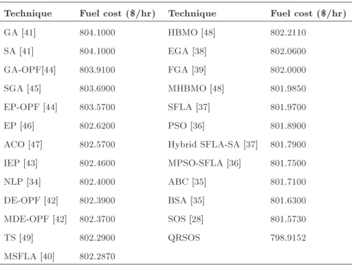
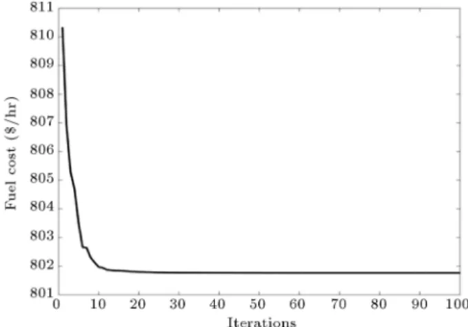
Test case 1 considers the minimization of QFC de-scribed by (16) as its objective. Simulation results are demonstrated in Table 1. The optimized fuel cost using QRSOS is attained as 798.9299 $/hr. A comparative study of Test case 1 as shown in Table 2 reveals that QFC obtained using the proposed technique is lower than the best value of 801.5733 $/hr, as obtained using SOS [28]. In addition, the result obtained using the proposed algorithm is better than that obtained using other recently applied algorithms, such as Backtracking Search Algorithm (BSA), Articial Bee Colony (ABC)

(8)

Table 1. Optimum control variable values for various test cases. Control variables Test case

1

Test case 2.1

Test case 2.2

Test case 3

Test case 4

Generator real power output (MW)

PG1 177 219.82 199.6 179.2 219.8

PG2 48.664 27.851 20 45 27.96

PG5 21.347 15.837 22.13 21.585 15.76

PG8 21.062 10 27 22.889 10

PG11 11.906 10 12.2 12.49 10

PG13 12 12 12.36 11.533 12

Generator output voltage (p.u.)

VG1 1.1 1.0813 1.0778 1.0746 1.0811

VG2 1.0881 1.05 1.05 1.05 1.05

VG5 1.0628 1.0232 1.0247 1.0244 1.0237

VG8 1.0694 1.0314 1.0366 1.0332 1.0316

VG11 1.072 1.1 1.0995 1.1 1.0999

VG13 1.1 1.05 1.0497 1.05 1.05

Transformer tap ratio

T6-9 0.98641 1.0998 1.0384 1.097 1.0997

T6-10 1.0111 0.9191 0.9926 0.9063 0.9182

T4-12 0.99402 0.9882 0.9949 0.9732 0.987

T27-28 0.96114 0.9634 0.9694 0.9584 0.9634

Total fuel cost ($/hr) 798.9299 825.2541 920.1125 801.7593 825.276

Real power loss (MW) 8.5836 12.1087 9.8959 9.3009 12.1128

Voltage stability index (p.u.) 0.1062 0.1292 0.1298 0.1279 0.1291

Voltage deviation (p.u.) 2.0338 0.5703 0.5686 0.6818 0.5775

Simulation time (s) 42.7342 87.5921 110.3562 120.4958 84.3752

Table 2. Comparative study of Test case 1.

Technique Fuel cost ($/hr) Technique Fuel cost ($/hr)

GA [41] 804.1000 HBMO [48] 802.2110

SA [41] 804.1000 EGA [38] 802.0600

GA-OPF[44] 803.9100 FGA [39] 802.0000

SGA [45] 803.6900 MHBMO [48] 801.9850

EP-OPF [44] 803.5700 SFLA [37] 801.9700

EP [46] 802.6200 PSO [36] 801.8900

ACO [47] 802.5700 Hybrid SFLA-SA [37] 801.7900 IEP [43] 802.4600 MPSO-SFLA [36] 801.7500

NLP [34] 802.4000 ABC [35] 801.7100

DE-OPF [42] 802.3900 BSA [35] 801.6300

MDE-OPF [42] 802.3700 SOS [28] 801.5730

TS [49] 802.2900 QRSOS 798.9152

(9)

Figure 2. Convergence characteristic of Test case 1.

optimization, Modied Shue Frog Leaping Algorithm (MSFLA), etc., as available in the literature listed in Table 2. Figure 2 portrays the convergence characteris-tic of Test case 1. The algorithm converged in less than twenty iterations, showing faster convergence than its predecessor does.

Test case 2: OPF problem considering VE. Test case 2.1

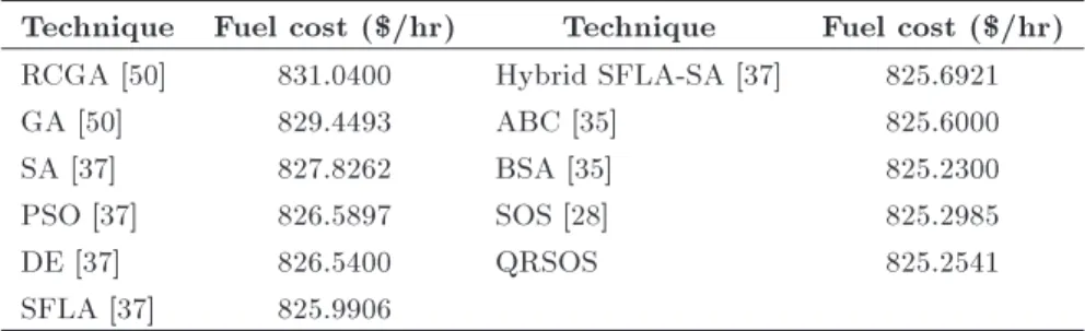
The result obtained for Test case 2.1 is provided in Table 1, which is derived by employing the generator cost coecients as given in Table 1 of Ref. [28]. The cost function for this objective is formulated using Eq. (17). It is seen that the obtained FC considering VE and using QRSOS algorithm is 825.2541 $/hr. Comparative study of this test case has been done, as

Figure 3. Convergence characteristic of Test case 2.1.

shown in Table 3. QRSOS provides better result than the previously obtained best value of 825.2985 $/hr, as achieved by SOS in [28]. Figure 3 depicts the convergence characteristics of this test case, and it is found to converge in less than thirty iterations. Test case 2.2

Results of this test case are given in Table 1. The attained FC is 920.1125 $/hr considering valve eect, using QRSOS algorithm, and generator cost coecients as provided in Table 6 of Ref. [28]. The cost function is described by Eq. (17). Comparative study is provided in Table 4, which substantiates that the proposed algorithm achieves better result than others to which it is compared. Figure 4 depicts the convergence characteristics of this case, and it is found to converge

Table 3. Comparative study of Test case 2.1.

Technique Fuel cost ($/hr) Technique Fuel cost ($/hr) RCGA [50] 831.0400 Hybrid SFLA-SA [37] 825.6921

GA [50] 829.4493 ABC [35] 825.6000

SA [37] 827.8262 BSA [35] 825.2300

PSO [37] 826.5897 SOS [28] 825.2985

DE [37] 826.5400 QRSOS 825.2541

SFLA [37] 825.9906

Table 4. Comparative study of Test case 2.2.

GA [51] 996.0369 ABC [53] 928.4370

GA-APO [51] 996.0369 PSO [54] 925.7581

NSOA [51] 984.9365 MSG-HS [54] 925.6410

ITS [43] 969.1090 IABC [55] 921.8265

TS-SA [43] 959.5630 IABC-LS [55] 921.8235

EP [43] 955.5080 BSA [35] 921.3570

IEP [43] 953.5730 SOS [28] 921.3288

(10)

Figure 4. Convergence characteristic of Test case 2.2.

in about thirty iterations, which is less than one-sixth of that required by SOS [28].

Test case 3: OPF considering POZ

Generator cost coecients as provided in Table 1 of Ref. [28] and QFC of Eq. (16) are considered. Obtained results of this test case are provided in Table 4. Table 5 provides a comparative study of this test case. QRSOS reduces objective function value to 801.7593 $/hr from the previously obtained best value of 801.8398 $/hr in [28]. Figure 5 depicts the convergence characteristics of this method that shows faster convergence in less than 45 iterations, which is nearly 36.36% of that required by SOS in [28].

Test case 4: OPF problem considering both VE and POZ

Generator cost coecients provided in Table 1 of [28] and cost function as described by Eq. (17) are consid-ered. The result of this case is tabulated in Table 1.

Comparative study of this objective is presented in Ta-ble 6, demonstrating competitiveness of the proposed algorithm to achieve lower cost. Figure 6 shows a faster convergence curve of this test case when compared to SOS [28].

GA [37] 809.2314 ABC [35] 804.3800

SA [37] 808.7174 BSA [35] 801.8500

PSO [37] 806.4331 SOS [28] 801.8398

SFLA [37] 806.2155 QRSOS 801.7593

Hybrid SFLA-SA [37] 805.8152

GA [37] 838.1727 ABC [35] 831.6500

SA [37] 836.5364 BSA [35] 826.3700

PSO [37] 835.4785 SOS [28] 825.3705

SFLA [37] 834.8165 QRSOS 825.2760

(11)

Control variables QRSOS QOTLBO [21] TLBO [21] MOHS [25] DSA [57]

PG1 51.244 51.3093 52.1027 52.5327 51.0945

PG2 79.999 80 79.9387 79.5432 80

PG5 50 49.9794 49.9617 49.8152 50

PG8 35 34.9959 34.5287 34.7403 35

PG11 30 29.9988 29.9721 29.7884 30

PG13 40 40 39.8304 39.948 40

VG1 1.1 1.087 1.0798 1.0754 1.0605

VG2 1.0981 1.0825 1.0742 1.0728 1.0566

VG5 1.0803 1.0632 1.0557 1.054 1.0378

VG8 1.0872 1.0707 1.0641 1.0637 1.0453

VG11 1.0712 1.0998 1.0976 1.0991 1.1

VG13 1.1 1.0989 1.0989 1.0967 1.0474

Shunt compensator injection (p.u.)

QC10 2.81E-05 0.0495 0.0498 0.0499 0.05

QC12 0.0499 0.0499 0.0498 0.0486 0.05

QC15 0.0498 0.0297 0.0497 0.0493 0.05

QC17 0.0498 0.0499 0.0498 0.0488 0.05

QC20 0.0421 0.0387 0.0403 0.0442 0.05

QC21 0.0499 0.05 0.0496 0.0499 0.05

QC23 0.0213 0.0273 0.0267 0.0411 0.0422

QC24 0.0312 0.05 0.0497 0.0499 0.05

QC29 0.0235 0.0207 0.0212 0.0317 0.0303

T6-9 1.0199 1.0309 1.0171 1.0022 1.0329

T6-10 0.9773 0.9024 0.9 0.9078 0.9993

T4-12 0.9864 0.9689 0.9681 0.9593 0.9913

T28-27 0.9741 0.9584 0.9527 0.9533 0.9786

Cost($/h) 967.0473 967.0371 965.7677 964.5121 967.6493

Transmission loss (MW) 2.8436 2.8834 2.9343 2.9678 3.0945

Voltage stability index (p.u.) 0.1074 0.1262 0.1264 0.1154 0.12604

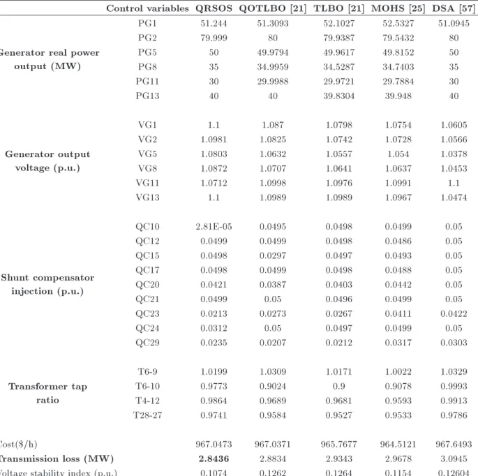
Test case 5: OPF problem with the objective of RTL minimization

Objective of this test case is formulated using Eq. (19). Table 7 lists the optimal control variables of this objective.

The suggested algorithm is capable of bringing down loss to 2.8423 MW, which is lower than that obtained using QOTLBO, TLBO, MOHS, and DSA in the literature. In addition, the result obtained using QRSOS is 1.42% lower than the previous best result of 2.8834 MW [21]. For this case, QRSOS took less than 35 iterations to converge, which is lower than that

(12)

Control variables QRSOS QOTLBO [21] TLBO [21] MOHS [25] DSA [57]

PG1 157.54 134.2408 76.788 92.6114 64.0725

PG2 40.938 61.8427 63.3618 67.5094 67.5711

PG5 15 15 45.7092 48.8891 50

PG8 10 10 33.8121 34.8663 35

PG11 29.994 29.9687 29.9842 29.7139 30

PG13 39.965 39.6304 37.4921 14.134 40

VG1 1.0705 1.0832 1.0601 1.0993 1.06

VG2 1.0444 1.0666 1.0463 1.0986 1.0549

VG5 0.9894 1.0426 1.043 1.0973 1.0316

VG8 1.0603 1.0389 1.0443 1.0998 1.0399

VG11 1.1 1.0938 1.0986 1.0984 1.0778

VG13 0.9695 1.0976 1.0926 1.0996 1.0709

QC10 0.0499 0.0492 0.0463 0.0499 0.0393

QC12 0.0499 0.0499 0.0487 0.0492 0.05

QC15 0.0498 0.0369 0.0497 0.0496 0.05

QC17 0.05 0.05 0.0426 0.0499 0.05

QC20 0.0499 0.0187 0.0437 0.05 0.05

QC21 0.05 0.0042 0.0434 0.0497 0.05

QC23 0.0485 0.0009 0.0193 0.0494 0.0406

QC24 0.0499 0.0005 0.0051 0.0494 0.05

QC29 0.0178 0.0011 0.0406 0.0496 0.0286

T6-9 1.0999 0.9288 0.9646 0.9027 0.9989

T6-10 1.0985 0.9 0.9602 0.9001 1.0046

T4-12 1.1 0.9442 0.92 0.9036 1.0368

T28-27 0.9002 0.9082 0.9256 0.9011 0.9792

Cost ($/h) 843.8153 844.1237 912.5914 895.6223 944.4086

Transmission Loss (MW) 10.0412 7.2826 3.7474 4.3244 3.24373

L-index (p.u.) 0.092613 0.0994 0.1003 0.1006 0.12734

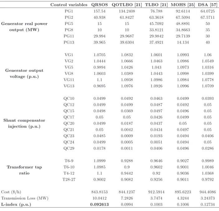
Test case 6: OPF for L-index minimization

This case considers lowering L-index value to improve voltage stability of the system using Eq. (20). Control parameters of this case are listed in Table 8.

It can be observed that the proposed methodology lowers the value of this objective function to 0.092613 p.u., which is the lowest of those obtained using QOTLBO, TLBO, MOHS, and DSA. In addition, it lowered the L-index value by 6.82% from the previous best-reported value of 0.0994 p.u. [21]. Figure 8 shows a quicker rate of convergence for this case, too. Test case 7: Voltage Deviation (VD) minimization This test case considers improving the load voltage prole of the system using Eq. (21). Optimal control

(13)

Control variables QRSOS NSGA-II [23]

PG1 0.5247

PG2 0.8

PG5 0.5

PG8 0.35

PG11 0.2978

PG13 0.4

VG1 1.0009 1.03

VG2 1.0016 1.03

VG5 1.0179 1

VG8 1.0084 1

VG11 0.9767 1.02

VG13 1.0059 1.04

QC10 0.9897

QC12 0.9697

QC15 0.9855

QC17 0.9758

QC20 0.0021

QC21 0.027

QC23 0.0499

QC24 0

QC29 0.05

T6-9 0.0448 1

T6-10 0.049 1.01

T4-12 0.0499 1

T28-27 0.0341 1.04

Voltage deviation (p.u.) 0.0798 0.38

Transmission loss (MW) 3.8676 5.3513

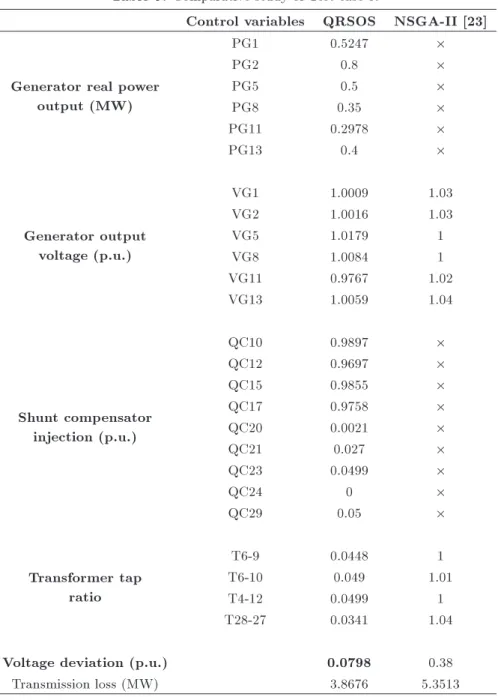
QRSOS lowered the VD value to 0.079866 p.u. by a high margin of 78.98% as compared to NSGA-II in [23]. The transmission loss is also reduced to a great extent. The algorithm converged within 25 iterations for this test case as observed in Figure 9.

5.2.2. Single-objective optimization for IEEE 118 bus test system

To check the competence of the oered algorithm in a large system, IEEE 118 bus test system is taken into consideration for studying dierent test cases. Data of the system are obtained from [58]. Penalty factors have been assigned to the objectives as per Eq. (14) to handle the possible constraint violations of this large

(14)

Figure 10. Convergence characteristic of Test case 8 obtained using QRSOS.

of [10000 100000], and tuning has been done in steps of 10000. Results of all penalty factors are not shown here for page limitations. Optimum results have been obtained for a penalty factor of 30000 assigned to the objectives, which are tabulated in the subsequent test cases:

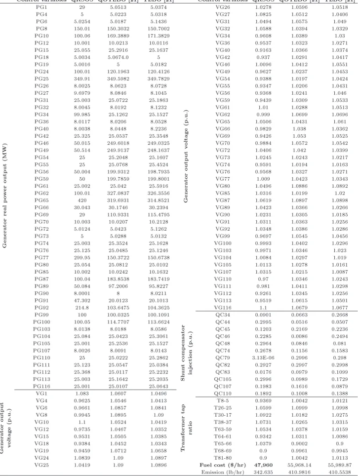
Test case 8: OPF problem for QFC minimization Optimal results are obtained for a penalty factor of 30000 assigned to the objective. The results and their comparisons are provided in Table 10.

As can be observed from Table 10, QRSOS eectively reduced the fuel cost by a large margin of 14.30% from 55,968.14 $/hr [21] to 47,960 $/hr. In ad-dition, it eectively reduced the emission from 410.9816 lb/hr [21] to a much lower value of 342.635 lb/hr in the case of single-objective optimization itself. It achieved better results than those of QOTLBO and TLBO in [21]. The proposed algorithm showed rapid convergence in less than 20 iterations, as seen in Figure 10.

Test case 9: OPF problem for real power transmission loss minimization

This test case minimized the real power loss occurring during transmission using Eq. (18). A penalty factor of 30000 assigned to the loss minimization objective gave optimum results, which are listed in Table 11.

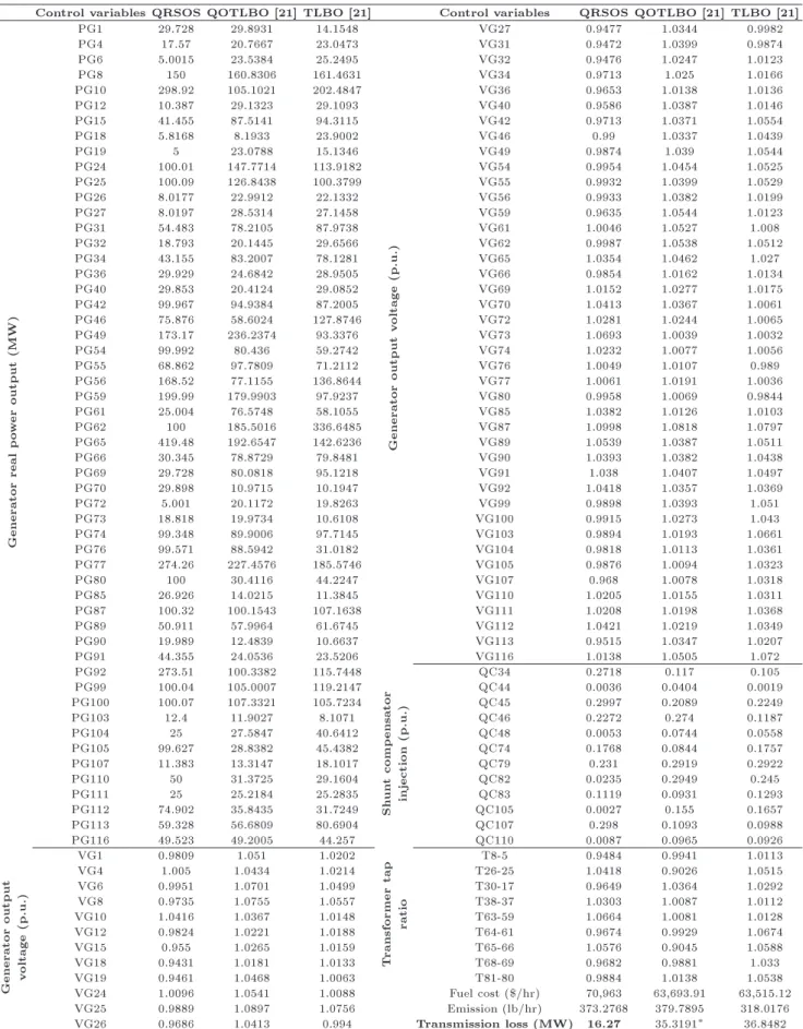
QRSOS is procient in reducing the transmission loss to 16.27 MW, nearly half of that of 35.3191 MW and 36.8482 MW obtained respectively by QOTLBO and TLBO, as reported in [21]. Simultaneously, it is also able to reduce the emission by 6.5127 lb/hr compared to that obtained by QOTLBO. Figure 11 shows rapid convergence in less than 20 iterations. Test case 10: OPF problem for minimizing L-index L-index of large IEEE 118 bus has been considered to improve voltage prole using Eq. (19). Since it is very dicult to maintain the voltage stability in

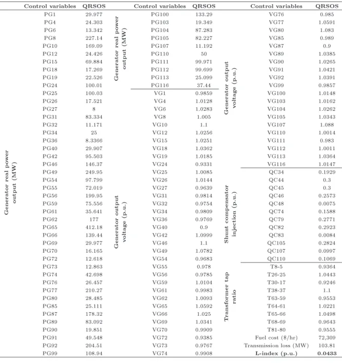
case of a large system, a penalty factor of 30000 has been assigned to the objective to handle inequality constraints. Optimum control parameters obtained for this test case are listed in Table 12.

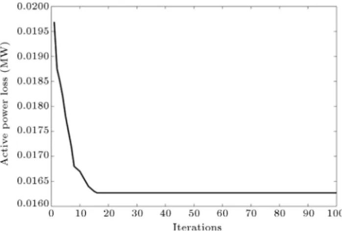
Optimal value of VSI is obtained as 0.0433 p.u., which denotes a stable system. Figure 12 shows the convergence characteristic of Test case 10. Convergence is achieved in less than 15 iterations.

Test case 11: OPF problem for emission minimization objective

This test case considers minimizing emission of pollu-tants to the atmosphere. The objective is formulated using Eq. (21). A penalty factor of 30000 assigned to the objective provided optimal results while eectively handling the constraints. Optimal parameters of this test case are listed in Table 13.

QRSOS provided the lowest emission value when compared to those obtained using QOTLBO and TLBO. It eectively reduced the emission from 176.1666 lb/hr in [21] to 164.5 lb/hr, i.e., by a margin of 6.62%. In addition, it reduced the fuel cost by 3.29% from 65,601.64 $/hr [21] and transmission loss by 7.58% from the previously reported best value of

(15)

Control variables QRSOS QOTLBO [21] TLBO [21] Control variables QRSOS QOTLBO [21] TLBO [21]

Generator

real

p

ow

er

output

(MW)

PG1 29 5.0513 5.0374

Generator

output

voltage

(p.u.)

VG26 1.0278 1.0596 1.0518 PG4 5 5.0223 5.0318 VG27 1.0825 1.0512 1.0406 PG6 5.0254 5.0187 5.1436 VG31 1.0494 1.0575 1.049 PG8 150.01 150.3032 150.7002 VG32 1.0588 1.0394 1.0329 PG10 100.06 169.3889 171.3829 VG34 0.9608 1.0389 1.03 PG12 10.001 10.0213 10.0116 VG36 0.9537 1.0323 1.0271 PG15 25.055 25.2916 25.1637 VG40 0.9163 1.0366 1.0374 PG18 5.0034 5.0674.0 5 VG42 0.937 1.0291 1.0417 PG19 5.0016 5 5.0182 VG46 1.0096 1.0412 1.0551 PG24 100.01 120.1963 120.4126 VG49 0.9627 1.0237 1.0453 PG25 349.91 349.5982 349.7829 VG54 0.9388 1.0197 1.0424 PG26 8.0025 8.0623 8.0728 VG55 0.9347 1.0206 1.0431 PG27 9.6979 8.0846 8.1045 VG56 0.9368 1.0241 1.046 PG31 25.003 25.0722 25.1863 VG59 0.9439 1.0309 1.0533 PG32 8.0045 8.0192 8.1232 VG61 1.01 1.0288 1.0513 PG34 99.985 25.1262 25.1527 VG62 0.999 1.0699 1.0696 PG36 8.0117 8.0206 8.0528 VG65 1.0506 1.0431 1.061 PG40 8.0038 8.0448 8.2236 VG66 0.9829 1.038 1.0362 PG42 25.325 25.0537 25.3548 VG69 0.9426 1.053 1.0525 PG46 50.015 249.6018 249.0325 VG70 0.9884 1.0572 1.0542 PG49 50.514 249.9137 248.1637 VG72 1.0406 1.042 1.0399 PG54 25 25.2048 25.1607 VG73 1.0245 1.0243 1.0217 PG55 25 25.0768 25.4524 VG74 0.9591 1.0194 1.0163 PG56 50.004 199.9312 198.7935 VG76 0.9568 1.0327 1.0271 PG59 50 199.7859 199.8001 VG77 1.009 1.0423 1.0343 PG61 25.002 25.042 25.5916 VG80 1.0496 1.0886 1.0892 PG62 100.01 327.0837 326.3556 VG85 1.0316 1.0199 1.02 PG65 420 319.6931 314.8521 VG87 1.0619 1.0897 1.0898 PG66 30.043 30.1746 30.2394 VG89 1.0423 1.0366 1.0266 PG69 29 110.9331 115.4795 VG90 1.0231 1.0305 1.0185 PG70 10.003 10.0207 10.2128 VG91 1.0311 1.0363 1.0256 PG72 5.0124 5.0423 5.1262 VG92 1.0348 1.0386 1.0286 PG73 5 5.0288 5.0132 VG99 0.9697 1.0545 1.0456 PG74 25.003 25.3524 25.1628 VG100 0.9993 1.0402 1.0296 PG76 25.125 25.0485 25.1246 VG103 0.9971 1.0346 1.023 PG77 299.95 150.3722 150.6738 VG104 1.0084 1.0297 1.019 PG80 25.054 25.0812 25.0102 VG105 1.0113 1.0278 1.0161 PG85 10.002 10.0242 10.1632 VG107 1.0315 1.0215 1.0087 PG87 100.04 183.8538 183.7419 VG110 0.97 1.0346 1.0243 PG89 50.084 97.2006 95.8227 VG111 0.981 1.0411 1.0298 PG90 8.0001 8 8.0211 VG112 0.9261 1.0345 1.0256 PG91 47.302 20.0123 20.1013 VG113 0.9519 1.0615 1.0501 PG92 214.8 103.6475 104.3625 VG116 1.1 1.0679 1.0677 PG99 100 100.0325 100.1091

Sh

un

t

comp

ensator

injection

(p.u.)

QC34 0.0901 0.0663 0.2668 PG100 100.05 114.7707 113.6624 QC44 0.2995 0.0516 0.0507 PG103 8.0138 8.0188 8.0586 QC45 0.1203 0.2169 0.2236 PG104 25.084 25.0423 25.3061 QC46 0.2285 0.0086 0.2494 PG105 25.001 25.2536 25.1527 QC48 0.2964 0.0846 0.081 PG107 8.0026 8.0091 8.0143 QC74 0.2678 0.1156 0.1583 PG110 25 25.0222 25.2862 QC79 3.13E-06 0.2996 0.298 PG111 25.123 25.0547 25.0384 QC82 0.2927 0.2997 0.2998 PG112 25.368 25.0117 25.2232 QC83 0.0176 0.0979 0.1099 PG113 25.003 25.1642 25.2035 QC105 0.2996 0.0989 0.1729 PG116 25.001 25.0107 25.0643 QC107 0.1983 0.1616 0.0879

Generator

output

voltage

(p.u.)

VG1 1.083 1.0607 1.0496 QC110 0.1892 0.1008 0.1388 VG4 0.9625 1.0546 1.0413

T

ransformer

tap

ratio

T8-5 0.9369 1.0042 1.0121 VG6 0.9661 1.0857 1.0841 T26-25 1.0599 1.0999 1.0998 VG8 0.9945 1.0895 1.09 T30-17 1.0922 1.0182 1.0275 VG10 1.1 1.0524 1.0419 T38-37 1.0731 1.0265 1.0315 VG12 0.9735 1.0467 1.0352 T63-59 1.0534 1.0378 1.0159 VG15 0.9531 1.0505 1.0385 T64-61 0.9342 1.0311 1.0086 VG18 0.9384 1.0452 1.0343 T65-66 1.0379 0.9002 0.9 VG19 0.9459 1.0712 1.0658 T68-69 0.9 0.9961 0.9945 VG24 1.0839 1.09 1.0897 T81-80 0.9 1.0042 1.0113 VG25 1.0419 1.09 1.0896 Fuel cost ($/hr) 47,960 55,968.14 55,989.87

(16)

Control variables QRSOS QOTLBO [21] TLBO [21] Control variables QRSOS QOTLBO [21] TLBO [21]

Generator

real

p

ow

er

output

(MW)

PG1 29.728 29.8931 14.1548

Generator

output

voltage

(p.u.)

VG27 0.9477 1.0344 0.9982 PG4 17.57 20.7667 23.0473 VG31 0.9472 1.0399 0.9874 PG6 5.0015 23.5384 25.2495 VG32 0.9476 1.0247 1.0123 PG8 150 160.8306 161.4631 VG34 0.9713 1.025 1.0166 PG10 298.92 105.1021 202.4847 VG36 0.9653 1.0138 1.0136 PG12 10.387 29.1323 29.1093 VG40 0.9586 1.0387 1.0146 PG15 41.455 87.5141 94.3115 VG42 0.9713 1.0371 1.0554 PG18 5.8168 8.1933 23.9002 VG46 0.99 1.0337 1.0439 PG19 5 23.0788 15.1346 VG49 0.9874 1.039 1.0544 PG24 100.01 147.7714 113.9182 VG54 0.9954 1.0454 1.0525 PG25 100.09 126.8438 100.3799 VG55 0.9932 1.0399 1.0529 PG26 8.0177 22.9912 22.1332 VG56 0.9933 1.0382 1.0199 PG27 8.0197 28.5314 27.1458 VG59 0.9635 1.0544 1.0123 PG31 54.483 78.2105 87.9738 VG61 1.0046 1.0527 1.008 PG32 18.793 20.1445 29.6566 VG62 0.9987 1.0538 1.0512 PG34 43.155 83.2007 78.1281 VG65 1.0354 1.0462 1.027 PG36 29.929 24.6842 28.9505 VG66 0.9854 1.0162 1.0134 PG40 29.853 20.4124 29.0852 VG69 1.0152 1.0277 1.0175 PG42 99.967 94.9384 87.2005 VG70 1.0413 1.0367 1.0061 PG46 75.876 58.6024 127.8746 VG72 1.0281 1.0244 1.0065 PG49 173.17 236.2374 93.3376 VG73 1.0693 1.0039 1.0032 PG54 99.992 80.436 59.2742 VG74 1.0232 1.0077 1.0056 PG55 68.862 97.7809 71.2112 VG76 1.0049 1.0107 0.989 PG56 168.52 77.1155 136.8644 VG77 1.0061 1.0191 1.0036 PG59 199.99 179.9903 97.9237 VG80 0.9958 1.0069 0.9844 PG61 25.004 76.5748 58.1055 VG85 1.0382 1.0126 1.0103 PG62 100 185.5016 336.6485 VG87 1.0998 1.0818 1.0797 PG65 419.48 192.6547 142.6236 VG89 1.0539 1.0387 1.0511 PG66 30.345 78.8729 79.8481 VG90 1.0393 1.0382 1.0438 PG69 29.728 80.0818 95.1218 VG91 1.038 1.0407 1.0497 PG70 29.898 10.9715 10.1947 VG92 1.0418 1.0357 1.0369 PG72 5.001 20.1172 19.8263 VG99 0.9898 1.0393 1.051 PG73 18.818 19.9734 10.6108 VG100 0.9915 1.0273 1.043 PG74 99.348 89.9006 97.7145 VG103 0.9894 1.0193 1.0661 PG76 99.571 88.5942 31.0182 VG104 0.9818 1.0113 1.0361 PG77 274.26 227.4576 185.5746 VG105 0.9876 1.0094 1.0323 PG80 100 30.4116 44.2247 VG107 0.968 1.0078 1.0318 PG85 26.926 14.0215 11.3845 VG110 1.0205 1.0155 1.0311 PG87 100.32 100.1543 107.1638 VG111 1.0208 1.0198 1.0368 PG89 50.911 57.9964 61.6745 VG112 1.0421 1.0219 1.0349 PG90 19.989 12.4839 10.6637 VG113 0.9515 1.0347 1.0207 PG91 44.355 24.0536 23.5206 VG116 1.0138 1.0505 1.072 PG92 273.51 100.3382 115.7448

Sh

un

t

comp

ensator

injection

(p.u.)

QC34 0.2718 0.117 0.105 PG99 100.04 105.0007 119.2147 QC44 0.0036 0.0404 0.0019 PG100 100.07 107.3321 105.7234 QC45 0.2997 0.2089 0.2249 PG103 12.4 11.9027 8.1071 QC46 0.2272 0.274 0.1187 PG104 25 27.5847 40.6412 QC48 0.0053 0.0744 0.0558 PG105 99.627 28.8382 45.4382 QC74 0.1768 0.0844 0.1757 PG107 11.383 13.3147 18.1017 QC79 0.231 0.2919 0.2922 PG110 50 31.3725 29.1604 QC82 0.0235 0.2949 0.245 PG111 25 25.2184 25.2835 QC83 0.1119 0.0931 0.1293 PG112 74.902 35.8435 31.7249 QC105 0.0027 0.155 0.1657 PG113 59.328 56.6809 80.6904 QC107 0.298 0.1093 0.0988 PG116 49.523 49.2005 44.257 QC110 0.0087 0.0965 0.0926

Generator

output

voltage

(p.u.)

VG1 0.9809 1.051 1.0202

T

ransformer

tap

ratio

T8-5 0.9484 0.9941 1.0113 VG4 1.005 1.0434 1.0214 T26-25 1.0418 0.9026 1.0515 VG6 0.9951 1.0701 1.0499 T30-17 0.9649 1.0364 1.0292 VG8 0.9735 1.0755 1.0557 T38-37 1.0303 1.0087 1.0112 VG10 1.0416 1.0367 1.0148 T63-59 1.0664 1.0081 1.0128 VG12 0.9824 1.0221 1.0188 T64-61 0.9674 0.9929 1.0674 VG15 0.955 1.0265 1.0159 T65-66 1.0576 0.9045 1.0588 VG18 0.9431 1.0181 1.0133 T68-69 0.9682 0.9881 1.033 VG19 0.9461 1.0468 1.0063 T81-80 0.9884 1.0138 1.0538 VG24 1.0096 1.0541 1.0088 Fuel cost ($/hr) 70,963 63,693.91 63,515.12 VG25 0.9889 1.0897 1.0756 Emission (lb/hr) 373.2768 379.7895 318.0176 VG26 0.9686 1.0413 0.994 Transmission loss (MW) 16.27 35.3191 _36.8482

_{The unit of the result obtained using QOTLBO for loss minimization in [21] is given as kW, whereas the real value comes as}

(17)

Table 12. Optimal parameter settings for Test case 10.

Control variables QRSOS Control variables QRSOS Control variables QRSOS

Generator

real

p

ow

er

output

(MW)

PG1 29.977

Generator

real

p

ow

er

output

(MW)

PG100 133.29

Generator

output

voltage

(p.u.)

VG76 0.985 PG4 24.303 PG103 19.349 VG77 1.0591 PG6 13.342 PG104 87.283 VG80 1.083 PG8 227.14 PG105 82.227 VG85 0.989 PG10 169.09 PG107 11.192 VG87 0.9 PG12 24.426 PG110 50 VG89 1.0385 PG15 69.884 PG111 99.971 VG90 1.0265 PG18 17.269 PG112 99.699 VG91 1.0421 PG19 22.526 PG113 25.099 VG92 1.0391 PG24 100.01 PG116 37.44 VG99 0.9857 PG25 100.03

Generator

output

voltage

(p.u.)

VG1 0.9859 VG100 1.0148 PG26 17.521 VG4 1.0128 VG103 1.0162 PG27 8 VG6 1.0283 VG104 1.0262 PG31 83.334 VG8 1.005 VG105 1.0343 PG32 11.171 VG10 1.1 VG107 1.088 PG34 25 VG12 1.0256 VG110 1.0014 PG36 8.3366 VG15 1.0251 VG111 0.983 PG40 29.907 VG18 1.0362 VG112 1.0011 PG42 95.503 VG19 1.0185 VG113 1.0364 PG46 146.37 VG24 0.9331 VG116 1.0147 PG49 249.95 VG25 1.0085

Sh

un

t

comp

ensator

injection

(p.u.)

QC34 0.1929 PG54 97.799 VG26 1.0144 QC44 0.3 PG55 72.019 VG27 0.9639 QC45 0.3 PG56 199.95 VG31 0.9814 QC46 0.2573 PG59 75.556 VG32 0.9754 QC48 0.0075 PG61 35.641 VG34 0.9809 QC74 0.1588 PG62 177 VG36 0.9769 QC79 0.2771 PG65 412.18 VG40 0.9 QC82 0.2923 PG66 139.44 VG42 1.0999 QC83 0.0084 PG69 29.977 VG46 1.1 QC105 0.2824 PG70 16.165 VG49 1.0782 QC107 0.0997 PG72 12.618 VG54 0.9683 QC110 0.1069 PG73 12.863 VG55 0.978

T

ransformer

tap

ratio

T8-5 0.9364 PG74 42.698 VG56 0.9785 T26-25 1.0443 PG76 26.457 VG59 1.0104 T30-17 0.9246 PG77 210.27 VG61 0.9983 T38-37 1.1 PG80 28.485 VG62 1.0093 T63-59 0.9553 PG85 25.111 VG65 1.0592 T64-61 1.0221 PG87 178.32 VG66 1.025 T65-66 1.0498 PG89 83.092 VG69 1.0341 T68-69 0.9643 PG90 19.851 VG70 0.9909 T81-80 0.9555 PG91 49.548 VG72 0.9385 Fuel cost ($/hr) 72,309 PG92 204.51 VG73 0.9767 Transmission loss (MW) 103.81 PG99 108.94 VG74 0.9908 L-index (p.u.) 0.0433

150.9366 MW [21], simultaneously. Figure 13 shows the convergence for this case.

5.2.3. Bi-objective results for IEEE 30 bus test system Nine dierent case studies have been carried out on the IEEE 30 bus test system for diverse MOO functions, and their pareto-fronts have been studied.

A Pareto optimal solution is dened as the nest solution set selected from numerous solution sets in which all objectives are equally compromised with respect to one another. Each solution set is dened as a non-dominated solution set. There can be an innite number of Pareto solution sets for a multi-objective

(18)

Table 13. Comparative study of Test case 11 for QRSOS.

Control variables QRSOS QOTLBO[21] TLBO[21] Control variables QRSOS QOTLBO[21] TLBO[21]

Generator

real

p

ow

er

output

(MW)

PG1 29 30 13.1937

Generator

output

voltage

(p.u.)

VG27 1.0882 1.0272 1.0426 PG4 11.361 29.9302 28.7162 VG31 1.0442 1.0338 1.0469 PG6 29.983 29.8782 18.4882 VG32 1.0657 1.0395 1.0453 PG8 150 299.8738 270.3844 VG34 0.9849 1.0375 1.0397 PG10 100.64 142.7617 264.8307 VG36 0.978 1.0249 1.0496 PG12 29.714 22.0728 29.1476 VG40 0.9348 1.0278 1.0571 PG15 91.021 44.0345 35.9218 VG42 0.9203 1.037 1.0694 PG18 5 5 5 VG46 0.9708 1.0373 1.0714 PG19 5 5.0111 5 VG49 0.9947 0.9948 1.0702 PG24 100 100.4435 100.4172 VG54 0.9451 1.049 1.0877 PG25 100 100.4082 100 VG55 0.9471 1.0261 1.0736 PG26 8.1201 26.9576 29.3547 VG56 0.9471 1.0526 1.0845 PG27 8.7412 12.112 28.2438 VG59 0.9598 1.0403 1.0883 PG31 67.54 97.9324 83.8513 VG61 1.012 1.031 1.0674 PG32 8 8.0141 8.0142 VG62 1.0163 1.0648 1.0663 PG34 25 25.0213 25.0202 VG65 1.0287 1.0456 1.0851 PG36 8 8 8.0134 VG66 0.9994 1.0304 1.0203 PG40 8 8 8.0283 VG69 0.9454 1.039 1.0349 PG42 32.46 99.6537 26.8744 VG70 0.9681 1.0406 1.042 PG46 249.95 179.4485 126.7132 VG72 1.053 1.0333 1.0233 PG49 50 50.0503 50.0483 VG73 1.0027 1.0143 1.0106 PG54 25 25.0728 25.1737 VG74 0.9424 1.0193 1.0072 PG55 25 25.0137 25.4218 VG76 0.951 1.0386 1.0291 PG56 50 50.0234 50.3506 VG77 1.0113 1.0629 1.0351 PG59 199.99 123.5961 132.1043 VG80 1.0464 1.0899 1.0842 PG61 38.07 84.2513 33.5485 VG85 1.0087 1.0146 1.0199 PG62 420 173.6788 254.15 VG87 1.063 1.0898 1.0871 PG65 80 80 80 VG89 1.0419 1.0428 1.0291 PG66 30 30.331 32.3293 VG90 1.0971 1.0415 1.0244 PG69 29 80.0753 107.9949 VG91 1.0322 1.0524 1.0381 PG70 10 10.2342 10.1963 VG92 1.0337 1.0537 1.0424 PG72 5 5.4008 10.5836 VG99 0.9764 1.0281 1.0883 PG73 5 5.6437 5.3809 VG100 1.0075 1.0706 1.0706 PG74 25 27.8556 25.5065 VG103 1.0086 1.0791 1.0743 PG76 25 27.6722 30.1247 VG104 1.0215 1.0631 1.043 PG77 240.34 272.0213 237.3293 VG105 1.0206 1.062 1.0447 PG80 84.397 70.0576 63.4527 VG107 1.0566 1.0513 1.0255 PG85 13.542 28.1374 19.2557 VG110 0.9757 1.0824 1.0256 PG87 179.01 181.63 299.4339 VG111 1.0213 1.0798 1.0492 PG89 113.86 144.6645 155.9003 VG112 0.9107 1.0865 1.0417 PG90 15.976 16.9528 19.6379 VG113 0.9662 1.0522 1.053 PG91 45.96 44.9324 41.5361 VG116 1.0521 1.0805 1.0739 PG92 196.58 147.4587 114.5003

Sh

un

t

comp

ensator

injection

(p.u.)

QC34 0.2999 0.1784 0.29 PG99 265.61 172 131.9728 QC44 0.1811 0.0462 0.0421 PG100 246.91 213.1142 175.3218 QC45 0.1032 0.2032 0.1844 PG103 11.754 19.4834 15.8526 QC46 0.0029 0.057 0.0233 PG104 74.106 80.2192 95.8003 QC48 0.0438 0.0766 0.0679 PG105 67.72 73.9628 83.2438 QC74 0.1116 0.1794 0.2857 PG107 14.257 19.7113 18.4581 QC79 0.0336 0.2993 0.297 PG110 48.915 48.6485 46.4433 QC82 0.3 0.2925 0.0962 PG111 31.689 85.3081 99.9002 QC83 1.57E-06 0.2999 0.287 PG112 83.836 83.2133 90.2355 QC105 0.0627 0.0487 0.197 PG113 33.722 67.1145 95.4081 QC107 0.1428 0.2225 0.2103 PG116 34.93 41.9238 29.7641 QC110 0.0007 0.0043 0.1421

Generator

output

voltage

(p.u.)

VG1 1.0597 1.0327 1.0191

T

ransformer

tap

ratio

T8-5 0.987 1.0119 1.017 VG4 0.9347 1.0254 1.0222 T26-25 0.9243 1.0989 1.0992 VG6 0.9593 1.072 1.0606 T30-17 1.0706 1.0134 1.0133 VG8 1.0014 1.0788 1.0775 T38-37 1.0145 1.0021 0.989 VG10 1.0859 1.0208 1.0258 T63-59 0.961 0.9761 1.0046 VG12 0.9831 1.0373 1.0333 T64-61 0.9181 1.0315 0.9929 VG15 0.9674 1.0342 1.0374 T65-66 1.0442 0.9612 0.9003 VG18 0.9569 1.0319 1.036 T68-69 0.9417 1.0321 1.0927 VG19 0.962 1.0449 1.0446 T81-80 0.9003 1.0116 1.0368 VG24 1.0996 1.0529 1.0583 Fuel cost ($/hr) 63,441 65,601.64 65,037.34 VG25 1.1 1.0766 1.078 Emission (lb/hr) 164.5 176.1666 182.9609 VG26 1.0156 1.0319 1.0311 Transmission loss (MW) 139.49 150.9366 188.5034

(19)

Test case 12: OPF problem for simultaneously minimizing QFC and RTL

This objective function is described using Eq. (23), and results are presented in Table 14. The comparative study, as depicted in Table 15, showed that the algo-rithm achieved better result than those obtained using

MO-DEA, QOTLBO, TLBO, MOHS, and NSGA-II in the literature. Compared to MO-DEA, QRSOS lowered the transmission loss from 5.5949 MW [64] by 1.69% to 5.5002 MW. However, at the same time, the total FC increased by a small margin of 0.071%. It was observed that VSI value improved simultaneously,

Table 14. Optimum control variable settings for dierent test cases for bi-objective functions.

Control variables Case12 Case13 Case14 Case15 Case16 Case17 Case18 Case19 Case20

Generator

real

p

ow

er

output

(MW)

PG1 1.2849 1.9356 2.1982 1.7688 1.9456 2.1981 1.7658 1.9249 2.1903 PG2 0.517 0.4513 0.2756 0.4873 0.4899 0.2842 0.4895 0.4677 0.2861 PG5 0.2967 0.2067 0.1609 0.2138 0.1862 0.1557 0.2154 0.1986 0.1688 PG8 0.35 0.1183 0.1 0.2114 0.1 0.1 0.2218 0.1425 0.1 PG11 0.2448 0.1 0.1 0.1186 0.1 0.0974 0.1191 0.1 0.1246 PG13 0.1958 0.12 0.1202 0.12 0.12 0.12 0.12 0.12 0.098

Generator

output

voltage

(p.u.)

VG1 1.1 1.1 1.081 1.1 1.1 1.0813 1.0485 1.0186 1.029 VG2 1.0904 1.0824 1.05 1.0873 1.0791 1.05 1.0289 1.0047 1.0282 VG5 1.0673 1.0566 1.0233 1.0615 1.0632 1.0234 1.0062 1.0181 1.0191 VG8 1.0773 1.064 1.0316 1.069 1.0562 1.0316 1.0049 1.0093 0.9959 VG11 1.0813 1.0926 1.0985 1.0768 1.1 1.1 0.9857 1.0001 1.0593 VG13 1.1 1.1 1.05 1.1 1.0582 1.05 0.9859 0.9976 1.0219

Sh

un

t

comp

ensator

injection

(p.u.)

QC10 0.0125 0.0125 | 0.05 0.05 | 0.05 0.0023 | QC12 0.0498 0.05 | 0.05 0.0427 | 0 0.0346 | QC15 0.05 0.0499 | 0.05 0.0446 | 0.05 0.05 | QC17 0.05 0.05 | 0.05 0.0367 | 0 0 | QC20 0.0429 0.0442 | 0.05 0.0066 | 0.05 0.05 | QC21 0.05 0.0499 | 0.0499 0.0447 | 0.0294 0.0434 | QC23 0.0183 0.022 | 0.0223 0.0233 | 0.045 0.0469 | QC24 0.0383 0.0402 | 0.0427 0.0144 | 0.05 0.05 | QC29 0.0234 0.0243 | 0.0201 0 | 0.02 0.0345 |

T

ransformer tap

ratio

T6-9 1.0102 1.0772 1.0997 1.0429 1.0368 1.1 1.002 1.0145 1.086 T6-10 0.9812 0.9032 0.9168 0.9493 1.0976 0.9127 0.9889 0.9712 0.9 T4-12 0.9756 0.9677 0.987 0.9712 1.0997 0.9832 0.9439 0.9652 0.9586 T27-28 0.9645 0.9579 0.9625 0.9574 0.9038 0.9572 0.968 0.9804 0.9419

Fuel cost ($/hr) 821.4655 833.3756 825.2938 799.0175 835.2983 825.4182 803.3138 842.5288 832.7439 Real power loss (MW) 5.5002 9.7887 12.0904 8.7768 10.7703 12.1405 10.0139 11.97 4 13.3898 Voltage stability index (p.u.) 0.1185 0.1081 0.129 0.1067 0.1072 0.1277 0.1446 11.974 0.135 Voltage deviation (p.u.) 1.6125 1.9877 0.5796 1.5026 0.9079 0.6268 0.0991 0.0832 0.1461 Simulation time (s) 59.6103 62.566 72.4231 52.352 68.203 76.5432 59.246 63.2024 61.0255

Table 15. Comparative study of Test case 12. Technique Fuel cost

($/hr)

Real power loss (MW)

Voltage stability index (p.u.)

MOHS [25] 832.6709 5.3143 NA

NSGA-II [23] 823.8875 5.7699 NA

TLBO [21] 828.5300 5.2883 0.1259

QOTLBO [21] 826.4954 5.2727 0.1255

MO-DEA [64] 820.8802 5.5949 NA

(20)

Figure 14. Pareto front for Test case 12.

thereby increasing the voltage stability margin. Fig-ure 14 depicts the Pareto-front obtained for the above objective.

Test case 13: OPF for simultaneously minimizing FC and RTL considering VE

Generator cost coecients provided in Table 1 of [28] are used for this objective described using Eq. (24). Results are presented in Table 14. The total FC attained using QRSOS is 833.3756 $/hr, which is 0.98% higher than that of Case 2.1, and the RTL is 9.7887 MW, which is 19.16% lower than that of Case 2.1. Figure 15 represents the Pareto front obtained for Test case 13. No existing results are available in the literature for doing comparative study.

Test case 14: OPF for minimizing FC along with RTL considering both VE and POZ

Generator cost coecients and the POZs, as provided in Table 1 of Ref. [28], are used in Eq. (24). Based on Table 14, it can be witnessed that total FC is 825.2938 $/hr and the RTL is 12.0904 MW. The total FC increased with a slight margin of 0.002% and RTL reduced by 0.18% when compared to single-objective minimization of Test case 4. Figure 16 represents the Pareto-front for this test case. No existing results are available in the literature for doing comparative study.

Test case 15: OPF for simultaneously minimizing QFC and L-index neglecting VE and POZ

This objective function is described using Eq. (25). Table 14 demonstrates results obtained for this bi-objective function. According to Table 16, QRSOS reduced the total QFC to 799.0175 $/hr, which is lower than those obtained using QOTLBO, TLBO, NSGA-II, and MOHS, and recently applied BSA and MO-DEA in the literature. Based on the comparison of the result with those of the latest algorithms such as BSA [63] and MO-DEA [64], it is observed that QRSOS

Table 16. Comparative study of Test case 15. Technique Fuel cost

($/hr)

Real power loss (p.u.)

Voltage stability index (p.u.)

Voltage deviation (p.u.)

MOHS [25] 799.9401 NA 0.1075 NA

NSGA-II [23] 800.3170 NA 0.1083 NA

TLBO [21] 799.8564 8.8592 0.1270 NA

QOTLBO [21] 799.3415 8.7050 0.1256 NA

BSA [63] 800.3340 8.4904 0.1259 1.9855

MO-DEA [64] 799.6912 8.602 0.1249 2.0498

(21)

lowers the QFC value by 0.0803%. Simultaneously, it can lower the VSI value to 0.1067 p.u. by 15.25% from the latest MO-DEA [64], thereby ensuring a stable system. Figure 17 represents the Pareto front for this bi-objective function.

Test case 16: OPF for simultaneously minimizing FC and VSI considering VE

Generator cost coecients as provided in Table 1 of [28] are used for this case described by Eq. (26). Results attained for this test case are tabulated in Table 14. Figure 18 shows the Pareto-front for this objective function. Overall, the FC for this bi-objective function came out to be 835.2938 $/hr and the VSI as 0.1072 p.u. The FC increased by a negligible margin of 1.21% and the VSI reduced by 17.70% when compared to single-objective minimization of Test case

Figure 19. Pareto front for Test case 17 obtained using QRSOS.

2.1. No existing results are available in the literature for comparison.

Test case 17: OPF for simultaneously minimizing FC and VSI considering VE and POZ

Generator cost coecients and POZs as provided in Table 1 of [28] are used for test case described by Eq. (26). Results obtained for this test case are demonstrated in Table 14. QRSOS achieved FC of 825.4182 $/hr and VSI of 0.1277 p.u. The total FC increased by a negligible margin of 0.017%, whereas the VSI improved by a margin of 1.08% when compared to single-objective minimization of Test case 4. Figure 19 represents the Pareto-front for this case. No existing results are available in the literature for comparison. Test case 18: OPF for minimizing QFC along with VD

This objective function is dened using Eq. (27). Results obtained for this test case are demonstrated in Table 14. VD obtained using QRSOS is 0.0991 p.u. which is 94.09% lower, and the total FC is 803.3138 $/hr which is 0.55% higher when compared to single-objective minimization of Test case 1. In addition, when compared to the recently applied techniques, such as BSA [63] and MO-DEA [64], it is observed from Table 17 that QRSOS lowers the FC as well as VD by 0.074% and 14.42%, respectively. Figure 20 depicts the Pareto front for this test case.

Test case 19: OPF to minimize FC along with VD considering VE

Generator cost coecients from Table 1 of [28] are

Technique Fuel cost ($/hr) Voltage deviation (p.u.)

BSA [63] 803.4294 0.1147

MO-DEA [64] 803.9116 0.1158

(22)

used for the case described using Eq. (28). Results obtained for this test case are demonstrated in Table 14. The total FC achieved using QRSOS is 842.5288 $/hr, which is 2.05% higher than that in Test case 2.1, and VD is achieved as 0.0832 p.u., which is 85.41% less than that obtained for single-objective minimization of Test case 2.1. Figure 21 represents the Pareto-front for this case. No existing results are available in the literature for comparison.

Test case 20: OPF for minimizing FC along with VD considering VE and POZ

Generator cost coecients and POZs in Table 1 of [28] are used for the case described using Eq. (28). Results are presented in Table 14. The total FC achieved using QRSOS is 832.7439 $/hr, which is 0.904% higher, and VD is achieved as 0.1461 p.u., which is 74.70% lower when compared to the single-objective minimization of Test case 4. Figure 22 represents the Pareto-front for this case. No existing results are available in the literature for carrying out a comparative study of this case, too.

Analyses of the aforementioned case studies prove the supremacy of the proposed technique over other

algorithms such as QOTLBO, TLBO, MOHS, NSGA-II, ABC, BSA, PSO, DE-PSO, EP, IEP, GA, IABC, SA, SFLA, MSFLA, NLP, TS, ACO, Hybrid SFLA-SA, and SOS available in literature for achieving an optimum solution to the OPF problem. QRSOS pro-duces superior solutions to other algorithms mentioned above for the cases studied. Pareto fronts obtained for each of the multi-objective functions depict solution sets well distributed in the search space, signifying a non-dominated solution.

6. Determining the best parameter settings for QRSOS

To determine the best parameter setting for QRSOS to deliver ecient results, population sizes of 10, 20, 30, 40, and 50 have been taken into consideration. For each population size, jumping rate JR is augmented from 0.1 to 0.9 in steps of 0.1, as shown in Table 18. Performance of QRSOS in Test case 4 is analyzed considering all the aforementioned combinations. Fifty dierent trials have been carried out with 100 iterations for each trial. Based on Table 18, it is observed that a population size of 30 and a Jumping Rate (JR) of 0.3 give the best fuel cost value of 825.2760 $/hr, which is less than previous best reported value of 825.3705 $/hr. 7. Statistical analysis of test results

Statistical analysis is done on 50 trial data sets to assess the performance of QRSOS. For this purpose, one trial data set, as obtained from the solution sets of the proposed algorithm, is tested using Wilcoxon Signed Rank Test (WSRT). A p-value (probability value) below 0.05 obtained from this test is considered as conclusive proof to counter the null hypothesis. p-values obtained using this test for Test cases 1-4 along with minimum, maximum, average values and standard deviation are tabulated below.

(23)

Table 18. Best parameter setting for QRSOS. Population

size Jumping Rate (JR)

0.1 0.2 0.3 0.4 0.5 0.6 0.7 0.8 0.9 1

10 826.5956 826.5543 826.5142 826.5492 826.6166 826.6473 826.6759 826.6921 826.7051 826.7149 20 826.4182 826.3762 826.3651 826.4960 826.6253 826.6395 826.6627 826.6863 826.7127 826.7248 30 825.5214 825.4075 825.2760 825.3153 825.3752 825.4242 825.4621 825.4875 825.5023 825.6942 40 825.5193 825.4695 825.4473 825.4752 825.4763 825.4954 825.5121 825.5274 825.5331 825.5781 50 825.5403 825.5325 825.4620 825.4854 825.4891 825.4902 825.5123 825.5179 825.5194 825.5344 Table 19. Statistical analysis of QRSOS for single objectives using Wilcoxon signed rank test against 50 trials.

Test

cases Minimum Average Maximum

No. of hits to minimum solution

Standard

deviation p-value

Case 1 798.9152 798.9439 799.0110 35 0.0443 1.12E-10

Case 2.1 825.2541 825.2866 825.4346 41 0.0700 3.66E-11

Case 2.2 920.1125 920.1514 920.3242 40 0.0828 5.96E-11

Case 3 801.7593 801.7668 801.8001 40 0.0160 5.96E-11

Case 4 825.2769 825.2785 825.2865 38 0.0045 6.92E-11

As observed in Table 19, p-value in every case is well below the desired value of 0.05 establishing statistical signicance of the results. Moreover, the standard deviation values obtained for QRSOS are much lower than those obtained by its predecessor [28] for all the cases.

Conclusion

This study aimed to introduce a novel technique des-ignated as quasi-reected symbiotic organisms search algorithm (QRSOS) to solve the OPF problem. The technique was successfully applied to the OPF problem to solve both single-objective and bi-objective func-tions. Twenty dierent test cases were solved with and without considering the VE and POZs. Outputs obtained using QRSOS were compared with those obtained by SOS, QOTLBO, TLBO, MOHS, NSGA-II, DE, and PSO; several other techniques are reported in the literature. Results obtained demonstrate the eciency and robustness of the oered technique in handling OPF problem for both small- and large-scale test systems. Results showed a remarkable improve-ment for QRSOS when compared to other available techniques. It passed the Wilcoxon signed rank test with very low p-values and established its statistical signicance. It was simultaneously observed that this algorithm acquired very fast convergence in all cases when matching other techniques. Henceforth, it may be deduced that QRSOS algorithm is promising, and there is a possibility for future research in this direction considering other aspects of power system.

Future scope

The proposed technique has eectively handled both linear and non-linear objectives. Since QRSOS was shown as able to solve the OPF problem successfully, it might be further applied to solve OPF, considering renewables and uncertainty due to load demands under dierent contingency scenarios.

Acknowledgement

The authors would like to acknowledge the lab facilities provided by the Electrical Engineering Department for carrying out the research work.

References

1. De Carvalho, E.P., dos Santos, A., and Ma, T.F. \Reduced gradient method combined with augmented Lagrangian and barrier for the optimal power ow problem", Applied Mathematics and Computation, 200(2), pp. 529-536 (2008).

2. Momoh, J.A., Adapa, R., and El-Hawary, M.E. \A re-view of selected optimal power ow literature to 1993. I. Nonlinear and quadratic programming approaches", IEEE Transactions on Power Systems, 14(1), pp. 96-104 (1999).

3. Santos, A.J. and Da Costa, G.R.M. \Optimal-power-ow solution by Newton's method applied to an augmented Lagrangian function", IEE Proceedings-Generation, Transmission and Distribution, 142(1), pp. 33-36 (1995).