Jackson_unc_0153D_14938.pdf

MONETARY POLICY IN A ZERO LOWER BOUND ENVIRONMENT

Laura E. Jackson

A dissertation submitted to the faculty of the University of North Carolina at Chapel

Hill in partial ful…llment of the requirements for the degree of Doctor of Philosophy in

the Department of Economics.

Chapel Hill

2014

Approved by:

Neville Francis

Michael Owyang

Richard Froyen

Eric Ghysels

ABSTRACT

LAURA E. JACKSON: MONETARY POLICY IN A ZERO LOWER BOUND

ENVIRONMENT.

(Under the direction of Neville Francis.)

In the wake of the Great Recession, the Federal Reserve lowered the federal funds rate

(FFR) target to zero and resorted to unconventional monetary policy. With the nominal FFR

constrained by the zero lower bound (ZLB), empirical monetary models cannot be estimated

as usual. First, in joint work with Neville Francis and Michael Owyang, we consider whether

standard models of monetary policy can be preserved without breaks. We consider whether

alternative policy instruments can be considered substitutes for the FFR over the ZLB period.

Furthermore, we construct a shadow rate via the methods proposed in Krippner (2012) and Wu

and Xia (2014) to proxy for the stance of policy. We ask whether the shadow rate is a su¢ cient

representation of the policy instrument or if the …nancial crisis requires other modi…cations.

We …nd that, if using a dataset that spans the pre-ZLB and ZLB environments, the shadow

rate acts as a fairly good proxy for monetary policy by producing impulse responses similar

to what we’d expect based on the non-ZLB benchmark. However, the linear model exhibits a

structural break at the onset of the ZLB and the shadow rate may be insu¢ cient for examining

the ZLB period in isolation.

Second, I describe the joint dynamics of bond yields, monetary policy and macroeconomic

variables within a no-arbitrage a¢ ne term structure framework while explicitly modeling the

ZLB using the shadow rate. I include data on the unemployment gap and in‡ation to build

a more comprehensive stance of policy, incorporating the in‡uences of unconventional

instru-ments introduced to combat the Great Recession. I …nd that shadow rate models incorporating

macroeconomic factors suggest a more negative shadow rate and a longer expected duration

allows the model to better capture the shift in policy focus towards targeting longer-term

yields. Finally, the shadow rate produces a proxy for the stance of policy that suggests the

unconventional programs achieved a substantial accommodation, in excess of that prescribed

ACKNOWLEDGMENTS

This project would not have been possible without the help and support of several people.

I am indebted to my advisors, Neville Francis and Michael Owyang for their guidance and

invaluable feedback. They have contributed immensely to my success in the economics

pro-fession. I would also like to thank each of the other members of my dissertation committee,

Richard Froyen, William Parke, and Eric Ghysels, whose comments and suggestions helped to

improve my work substantially. I bene…tted from conversations with Anusha Chari, Jonathan

Willis, Lutz Hendricks, and the research department of the Federal Reserve Bank of Kansas

City. Furthermore, I thank the participants of the Macro-Money seminar at UNC-Chapel Hill,

and the 22nd Symposium of the Society for Nonlinear Dynamics and Econometrics for their

constructive feedback. I completed part of this work as a CSWEP (Committee on the Status

of Women in the Economics Profession) Summer Economics Fellow in the Research Division

of the Federal Reserve Bank of Boston and as a Dissertation Intern at the Research Division

of the Federal Reserve Bank of Kansas City. These opportunities contributed immensely to

my progress as a research economist and I am grateful for their hospitality.

Lastly, I could not have completed the journey through graduate school without the

un-conditional love and support of my family and friends. I thank my parents, Jay and Sheri, for

their encouragement and always trusting and believing in me, even when my own belief may

have waivered. My brother, JJ, has always given me inspiration to see the best in the world

and this consistent focus helped me to persevere through the most di¢ cult of times. Finally,

I thank Eric for always supporting me in pursuit of my dreams and for reminding me of what

TABLE OF CONTENTS

LIST OF TABLES

. . . viii

LIST OF FIGURES

. . . .

ix

1

FOREWORD

. . . .

1

1.1

Literature on Monetary Policy in a ZLB Environment . . . .

4

2

MONETARY POLICY ANALYSIS AFTER THE FINANCIAL CRISIS

.

7

2.1

Introduction . . . .

7

2.2

The Benchmark Speci…cation . . . .

9

2.2.1

Testing for Parameter Instability . . . .

12

2.3

Monetary Policy at the ZLB . . . .

13

2.3.1

Adding Alternative Monetary Instruments . . . .

13

2.3.2

Shadow Short Rates . . . .

15

2.3.3

Model Performance . . . .

20

2.3.4

The Bottom Line . . . .

21

2.4

Conclusions . . . .

22

3

MONETARY POLICY AND MACRO FACTORS AT THE ZLB

. . . . .

24

3.1

Introduction . . . .

24

3.2

Empirical Methodology

. . . .

29

3.2.1

Central Bank Policy Rate and Observable Macroeconomic Indicators . .

30

3.2.2

Macro-Finance Model . . . .

34

3.2.3

Macro-Monetary Model . . . .

35

3.2.4

Finance Model . . . .

37

3.3

Data . . . .

38

3.4

Estimation

. . . .

39

3.5

Shadow Rate Estimation Results . . . .

40

3.5.1

Macro-Finance Model . . . .

40

3.5.2

Macro-Monetary Model . . . .

41

3.5.3

Finance Model . . . .

42

3.5.4

In-Sample Yield Curve Forecasting . . . .

43

3.6

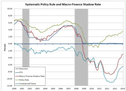
Macro-Finance Shadow Rate and Policy Rules

. . . .

46

3.7

What Do Markets Expect?

. . . .

48

3.8

Conclusion

. . . .

51

A TECHNICAL APPENDIX

. . . .

53

A.1 Standard GATSM Methodology . . . .

53

A.1.1 Estimation of Parameters with the Kalman Filter

. . . .

54

A.2 Constructing the Shadow Term Structure . . . .

55

A.3 MCMC Algorithm for Drawing Parameters and Latent Factors . . . .

59

A.3.1 Likelihood . . . .

60

A.3.2 Drawing the Latent Factors (

f

)

. . . .

61

A.3.3 Drawing the State Transition VAR Dynamics . . . .

61

A.3.4 Drawing the Risk Neutral Dynamics . . . .

62

A.3.5 Drawing the Observable Dynamics . . . .

63

A.3.6 Estimation of the Short Rate Dynamics . . . .

63

A.4 Extended Kalman Filter

. . . .

64

B TABLES AND FIGURES

. . . .

67

LIST OF TABLES

B.1 Bayes Factor Comparison for Parameter Instability . . . .

67

B.2 Kullback-Leibler Divergence . . . .

68

B.3 Prior Parameterization for MCMC Estimation Algorithm . . . .

68

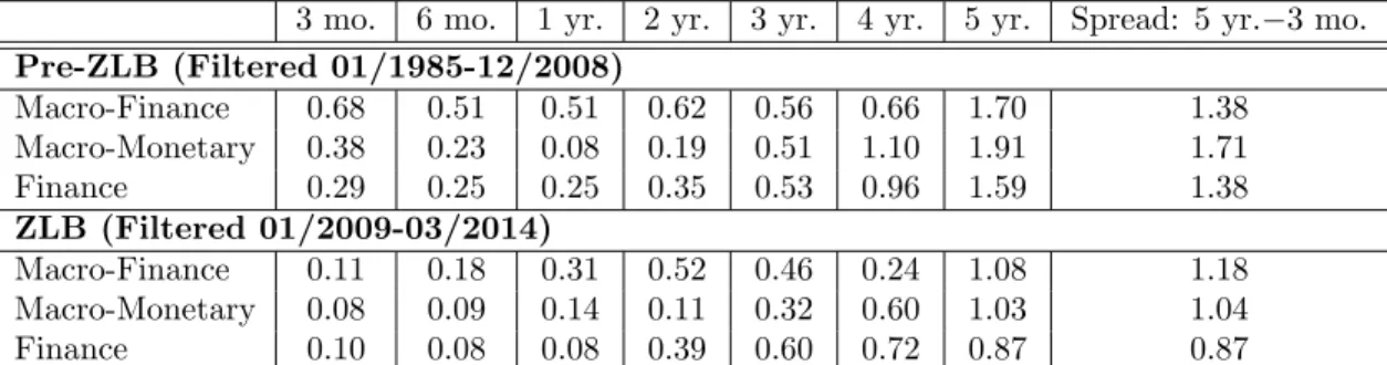
B.4 Root mean-squared errors: model-implied yields versus observed data

. . . . .

69

LIST OF FIGURES

B.1 Impulse Responses with the Federal Funds Rate: 1960-2013 . . . .

71

B.2 Impulse Responses with the FFR and Policy Announcements: 1960-2013 . . . .

72

B.3 Quarterly Federal Funds Rate and Estimated Shadow Rates: 2006 - 2013 . . .

73

B.4 Impulse Responses Over the Full Sample with Shadow Rates: 1960-2013 . . . .

74

B.5 Impulse Responses in the ZLB Environment with Shadow Rates: 2008-2013 . .

75

B.6 Monthly Macro Data 1985-2014 . . . .

76

B.7 Plot of E¤ective Federal Funds Rate and Filtered Shadow Rates: 1985-2014 . .

76

B.8 E¤ective Federal Funds Rate and Three-Factor Shadow Rates: 2000-2014 . . .

77

B.9 Macro-Finance Shadow Rate Model Components . . . .

77

CHAPTER 1 FOREWORD

The global recession of 2008-2009, driven mainly by the …nancial crisis in the U.S., triggered

unprecedented responses in both …scal and monetary policy. Traditional economic theory

suggests that, in normal times, the short-term interest rate (Federal Funds rate) provides a

clear indicator of the stance of monetary policy and allows consumers and investors to discern

the intent of the central bank. The Federal Reserve targets a lower (higher) policy rate in order

to stimulate (contract) the economy in response to business cycle ‡uctuations. To combat the

recent recession, the Fed lowered short-term interest rates to near-zero levels to make it easier

for businesses and households to borrow and invest. Nominal interest rates cannot become

negative if currency exists since money pays zero interest and investors would rather hold

cash than earn a negative return. Therefore, the Federal Funds rate (henceforth referred to

as FFR) being near zero for an extended period forced the adoption of alternative policies to

drive economic growth.

The Fed introduced programs such as quantitative easing and large-scale purchases of

long-term assets, including mortgage-backed securities. In doing so, the Fed sought to lower interest

rates in the housing market and on other long-term …nancial assets to ease borrowing costs and

encourage investment. These unconventional programs represent a diversion from traditional

policy as described by models of monetary economics. Therefore, these models must either

include more policy instruments or introduce some sort of transitional structural change in the

operating procedures of the Fed during this time.

Economists are tasked with rede…ning the “policy rate” to absorb the e¤ects of these

alternative programs and thus give a more accurate description of the stance of monetary

policy. To this end, my research expands upon current models of estimating a shadow policy

central bank. Although market interest rates are necessarily nonnegative, the shadow rate

may become negative during periods of extremely loose monetary policy. One can construct

this shadow rate by estimating a model of the term structure of interest rates, anchored by

the Fed’s policy rate. Typical term structure models do not control for the inability of

short-term rates to fall below zero. This dissertation estimates various models accounting for this

constraint and analyzes how the alternative programs a¤ected the true and perceived stances

of monetary policy throughout the Great Recession.

In Section 1.1, I summarize the existing literature on measuring monetary policy at the

ZLB. Many studies have sought to discern the e¤ects of unconventional policy instruments by

conducting event-studies around their introduction.

In Chapter 2, joint work with Neville Francis and Michael Owyang, we consider whether

the standard empirical model of monetary policy can be preserved without breaks. We test

whether alternative policy instruments (e.g., the size of the balance sheet) can be considered

substitutes for the FFR over the ZLB period. That is, we ask whether, during the ZLB

period, there exists a relationship between the FFR and the alternative instruments so that

the standard monetary policy vector autoregression (VAR) dynamics can be preserved. We

propose controlling for the size of the Fed’s balance sheet and information on alternative

policy announcements to represent policy action during the ZLB period from 2009:Q1 through

2012:Q4. We included these additional variables in a VAR to determine whether we could

produce the same impulse responses of key macroeconomic indicators in the ZLB environment

as those generated in baseline post-WWII macroeconomic models. We found that the balance

sheet and policy events appear to produce an accurate representation of policy during this

period but may be ine¢ cient to use for future empirical work once we return to a normal,

non-ZLB environment and these policies are no longer in use. Next, we test whether the shadow

rate is a su¢ cient representation of the policy instrument or if the …nancial crisis requires

other modi…cations to the monetary model. We …nd that the shadow rate acts as a fairly good

proxy for monetary policy, if using a dataset that spans the pre-ZLB period throughout the

ZLB environment, and produces impulse responses of macro indicators similar to what we’d

for examining the ZLB period in isolation.

In Chapter 3, I expand this framework using economic indicators to establish the

rela-tionship between interest rates, monetary policy and macroeconomic ‡uctuations. I construct

a macro-…nance shadow rate model which extends the current shadow rate methodologies to

incorporate information on key macroeconomic indicators when constructing the perceived

stance of policy through the ZLB period. An expansive literature has developed which

recog-nizes the value of modeling the macroeconomy and …nancial markets together. The Fed sets

policy to in‡uence the availability of money and credit, thus establishing a direct channel

link-ing policy and …nancial market activity. Furthermore, actions of the Federal Open Markets

Committee (FOMC) are closely watched by …nancial markets while the FOMC itself extracts

information about the current state of the economy from interest rates before setting policy.

I construct three di¤erent versions of the shadow rate model, di¤ering in the extent to which

I allow the macro data to in‡uence term structure dynamics. First, in the “Macro-Finance

model”, I incorporate macro ‡uctuations as factors which directly in‡uence the shadow

short-term rate. According to this interest rate reaction function, the Fed sets monetary policy in

response to the current state of the economy and makes adjustments according to changes in

in‡ation and real activity. Including a latent factor to represent unobserved shocks to policy, I

anchor the term structure with a shadow short rate directly in‡uenced by macro ‡uctuations.

Secondly, in the “Macro-Monetary model”, I restrict the observable dynamics to describe the

shadow rate as only a function of latent …nancial factors, prohibiting the macro factors from

directly feeding back into the term structure. Based upon a standard monetary VAR, I model

the unemployment gap and in‡ation as responding to lagged policy rates. I extract additional

information from observations on macro indicators each period to …lter the path of the shadow

rate. Finally, for comparison to existing studies, I construct the shadow rate using only interest

rate data in the “Finance model”.

The results suggest that it is inappropriate to use only the Federal Funds rate to represent

policy in a dataset which spans both normal and ZLB environments. The shadow rate model

produces a more comprehensive measurement of monetary policy at the ZLB by capturing how

Furthermore, utilizing macro data in a reactionary way, as in the Macro-Monetary model,

is more appropriate than models allowing the macro ‡uctuations to feedback into the term

structure. Finally, the shadow rate produces a proxy for the stance of policy that suggests

the unconventional policy programs achieved a substantial accommodation, in excess of that

prescribed by a standard policy rule.

1.1

Literature on Monetary Policy in a ZLB Environment

Bernanke & Reinhart (2004) discuss various strategies for stimulating the economy facing

the ZLB when the short-term policy rate cannot be lowered any further. These strategies

include the use of forward guidance to assure investors that the Fed will hold short-rates low

for a longer period into the future than may be expected by …nancial markets, changing the

composition of the Fed’s balance sheet to adjust the relative supplies of securities of di¤erent

maturities available in the market, and quantitative easing to increase the size of the balance

sheet beyond that required to keep the policy rate near zero. The use of these alternative tools

signals to the public that the Fed can still enact e¤ective policy even when traditional policy

in not applicable. In related work, Bernanke et al. (2004) use a variety of empirical …nance

methods to gauge the potential e¤ectiveness of unconventional monetary policy programs in

a ZLB environment. The authors conduct an event-study analysis to measure the response

of …nancial markets to various central bank announcements. Also, they estimate di¤erent

no-arbitrage VAR models of bond yields using only observable macroeconomic factors to describe

the term structure. In the VAR models, they establish a direct link between the term structure

and observable economic conditions which makes it easy to see how unconventional policies

can be e¤ective. They …nd that policymakers still can in‡uence expectations of future policy

even when the current FFR falls to zero. By convincing …nancial markets that it will maintain

low policy rates for longer than expected, the Fed can reduce long-term interest rates and

stimulate real economic activity.

Williams (2010) discusses the implications of extended ZLB episodes for the e¢ cacy of

monetary policy. In the wake of severe, prolonged recessions accompanied by de‡ation,

monetary authority must seek alternative sources of stimulus. In response to a sluggish

recov-ery and de‡ationary scare, the Fed incorporated recommendations from mainstream research

and cut the policy rate to a very low level. Once exhausting its traditional policy instrument,

the FOMC used policy statements to communicate expectations for the contour of the future

path of policy. Also, the FOMC communicated its patience in removing policy accommodation

by stating that it anticipated economic conditions would warrant exceptionally low levels of

the FFR for an extended period. This language remained vague enough to avoid committing

to speci…c values of the policy rate and to avoid forcing market expectations to abide by a

particular timeline.

A key motivation of the large-scale asset purchase (LSAP) programs was to lower interest

rates paid by households and businesses to support consumption and investment spending.

Wright (2011) conducts an event-study analysis to determine how …nancial markets responded

to the FOMC news. After November 2008, estimated monetary policy shocks signi…cantly

a¤ected 10-year Treasury yields and long-maturity corporate bond yields but the e¤ects lasted

only a few months. Furthermore, policy shocks had a small e¤ect on 2-year Treasury yields.

The existence of a relationship between aggregate demand and long-term interest rates would

suggest that unconventional monetary policy at the ZLB had a stimulative e¤ect on the

econ-omy, albeit rather modest.

Swanson & Williams (2013) measure the e¤ects of the ZLB on interest rates of all

matu-rities by examining the sensitivity of interest rates to announcements about macroeconomic

conditions. Over the period from 2008 through 2010, yields on Treasuries with more than one

year to maturity were very responsive to macro news, indicative of how monetary and …scal

policy were as e¤ective as in normal times. By late 2011, once the ZLB environment had

per-sisted for an extended period, the sensitivity fell considerably and almost entirely muted the

responsiveness of interest rates to macro news. The authors o¤er the explanation that market

participants may have begun to expect the FFR target to be above zero four quarters in the

fu-ture so medium- and long-term yields ceased to respond to cyclical news. The unconventional

policy actions of the Fed may also have helped to o¤set the e¤ects of news announcements.

constraint by promising accommodative monetary policy in the future once the constraint no

longer binds.

Bauer (2011) performs another event-study analysis of U.S. policies implemented in the

ZLB environment. He constructs a simple three-factor GATSM that accounts for heterogeneity

of shocks to interest rates stemming from di¤erent types of macro news announcements and

policy surprises. Daily interest rate changes are driven mostly by news announcements due to

changes in expectations of future policy rates and unexpected changes in risk-premia. Also,

news about in‡ationary pressures can move the long end of the term structure. The event-study

of Gagnon et al. (2011a) examines changes in interest rates within one-day windows around

o¢ cial communications regarding asset purchases. The authors …nd evidence that LSAP’s led

to economically meaningful and persistent reductions in longer-term rates. This was likely

driven by lower risk premiums and lower expectations of future short rates. Furthermore,

Neely (2013) …nds that announcements of LSAP’s by the Fed had substantial global e¤ects

and reduced international long-term yields and the spot value of the dollar.

This further

suggests that central banks can enact e¤ective monetary policy even when constrained by the

CHAPTER 2 MONETARY POLICY ANALYSIS AFTER THE FINANCIAL

CRISIS

2.1

Introduction

Since the onset of the Financial Crisis and Great Recession, monetary policy in the U.S. and

around the world has taken unprecedented measures in an e¤ort to stimulate the economy.

The Federal Reserve, for example, lowered its primary policy instrument— the federal funds

target— essentially to zero.

At that point, this instrument became ine¤ective due to the

nominal bound at zero and the Fed was forced to resort to unconventional monetary policy.

From the standpoint of academics, this period presents an important problem for assessing

the e¤ects of monetary policy. Many monetary models use the e¤ective nominal fed funds

rate as the primary policy instrument. With the nominal funds rate constrained by the zero

lower bound (ZLB) for an extended period, empirical monetary models cannot be estimated

as usual.

The empirical literature o¤ers a number of remedies. First, we could treat the ZLB period

as special, using either breaks or dummies to represent changes in economic relationships.

Second, we could include alternative policy instruments, such as the size of the balance sheet or

dummies representing the implementation of unconventional policies. These two alternatives

1

Friedman (2010) describes a detailed timeline of the sequence of steps taken by the Fed along with signi…cant market events. Williams (2011) presents a review of the unconventional monetary policy tactics employed to combat the …nancial crisis.

2_{Unconventional monetary policy used in the U.S. included quantitiative easing (QE), large scale asset} purchases (LSAPs), and forward guidance. Walsh (2010) discusses the channels through which quantitative easing could stabilize the economy. Wright (2011) analyzes how long-term interest rates respond to LSAP’s in a ZLB environment. Gagnon et al. (2011b) present the mechanisms through which these purchases a¤ect the overall macroeconomy. Campbell et al. (2012) discuss the e¤ects of forward guidance.

3

have the disadvantage of increasing the number of estimated parameters for a period that,

presumably, represents a short sample. Third, we could replace the FFR as the conventional

stance of monetary policy with a proxy that is allowed to violate the ZLB and that captures

the e¤ects of both conventional and unconventional policy.

Since the …nancial crisis, academics have proposed such measures of the accommodation in

monetary policy when the short rate is at the zero lower bound. Recently, Krippner (2012) and

Wu & Xia (2014) have used the shadow rate methodology to construct alternative measures

of the stance of policy. Krippner (2012) builds on Black (1995) and Gorovoi & Linetsky

(2004), modeling interest rates as options by calculating the value of a call option to hold

cash.

The modi…cations in Krippner (2012) generate closed-form solutions for bond prices

and yields. Rather than describing yields in a ZLB environment directly, Wu & Xia (2014)

construct an analytical approximation of forward rates in discrete time. This allows for a more

straightforward estimation approach than the other shadow rate methodologies and produces

closed-form expressions for the shadow forward rates. Both models calculate a shadow

short-term interest rate which would be seen in …nancial markets if the cash option did not exist. In

principle, the Fed may have dropped the fed funds rate further if not for the nominal bound

at zero. The shadow rate has been considered a proxy for the stance of monetary policy in an

environment in which the zero lower bound is binding. From this foundation one can develop

a full model of the shadow term structure based upon the shadow short rate depicting the

fundamental policy objectives.

Most previous empirical models of the e¤ects of policy were linear. If these shadow short

rates are proper measures of the monetary accommodation, the underlying model would, in

the best of worlds, still be linear and consistent across sub-periods. In this paper, we compare

some of these new measures of monetary policy. We consider whether the standard empirical

4

model of monetary policy can be preserved without breaks by using these measures. That is, we

ask whether, during the ZLB period, there exists a linear relationship between the alternative

instruments and standard macroeconomic variables so that the standard linear VAR can be

preserved.

The question going forward is whether these new alternative shadow short rates are su¢

-cient representations of monetary policy or if the …nancial crisis requires other modi…cations

to the monetary model. We ask the following questions: (1) How large are the biases in the

estimated impulse responses if one uses the FFR for the full sample? (2) Does adding policy

dummies and the balance sheet of the Fed mitigate these biases? (3) Does replacing the

e¤ec-tive funds rate a shadow short rate mitigate these biases? (4) Which shadow short rate does

a better job at mitigating these biases?

We …nd that the shadow rate acts as a fairly good proxy for monetary policy, if using

a dataset that spans the pre-ZLB period throughout the ZLB environment, by producing

impulse responses of macro indicators similar to what we’d expect based on the post-WWII,

non-ZLB benchmark. However, the linear model exhibits a signi…cant structural break at the

onset of the ZLB and the shadow rate may still be insu¢ cient for examining the ZLB period

in isolation.

The balance of the paper is organized as follows: Section 2.2 establishes the benchmark

speci…cation using standard empirical models to describe Fed policy in a normal, pre-ZLB

environment.

Section 2.3 examines how we can model some of the actions taken by the

Fed at the zero lower bound in these standard models. In this section, we consider whether

standard empirical models of monetary policy can be salvaged, either using new measures of

policy, allowing for breaks in the e¤ects of policy, and/or accounting for unconventional policy

instruments. Finally, Section 2.4 concludes.

2.2

The Benchmark Speci…cation

The short rate— often, an overnight rate— is one of the primary instruments for conducting

monetary policy. When adverse shocks are large, monetary accommodation can drive the short

zero since agents can substitute out of bonds into cash. This feature of nominal interest rates

can prevent a proper evaluation of the stance of monetary policy when the short rate is at or

near zero and other instruments must be relied upon to conduct policy. In this section, we

estimate a standard monetary VAR for the pre-crisis period (1960:I-2007:IV) and then naïvely

extend the analysis with data for the …nancial crisis period.

Before we can determine whether empirical models of monetary policy have changed, we

must …rst establish a baseline. We estimate a quarterly four-variable VAR(4) in output,

in-‡ation, commodity prices, and a policy instrument.

For the baseline model, we include the

e¤ective FFR as the policy instrument:

Y

=

A

(

L

)

Y

+

"

;

where

A

(

L

)

is a polynomial in the lag operator,

"

N

(0

;

)

, and we suppress the constant

and any trends for notational simplicity. The monetary shock is identi…ed by assuming that

FFR can react to macro variables but the macro variables cannot contemporaneously react to

shocks to the FFR. Partitioning

A

(

L

)

into blocks will facilitate exposition: Let

X

represent

the three macro variables of interest and

R

represent the FFR. Then, we can rewrite the VAR

as:

2

6

4

X

R

3

7

5

=

2

6

4

A

X

₍

_L

₎

_A

₍

_L

₎

A

₍

_L

₎

_A

₍

_L

₎

3

7

5

2

6

4

X

R

3

7

5

+

2

6

4

"

"

3

7

5

;

where

A

(

L

)

represents the e¤ects of changes in the lagged macro variables on each other,

A

(

L

)

represents the e¤ects of policy on the macro variables,

A

(

L

)

represents the

feed-back from macro variables to policy, and

A

(

L

)

represents the possible persistence in FFR.

The baseline data sample covers the period from 1960:I to 2007:IV, which starts after the

Korean War price control period and ends prior to the …nancial crisis and generally corresponds

with the standard VAR used for monetary analysis prior to the FFR hitting the zero lower

bound.

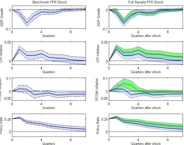
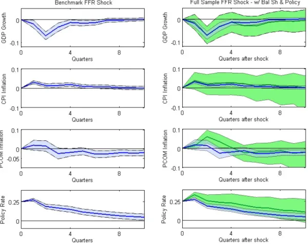
The …rst column of Figure B.1 shows the impulse responses for the VAR(4) outlined above

using the e¤ective nominal FFR as the policy instrument and data for the period ending in

2007:IV. The responses shown are to a 25 basis point shock to the e¤ective nominal FFR

ordered last in the VAR and identi…ed using the Cholesky decomposition. The responses are

computed for each draw of the sampler, generating the posterior coverage. The plots show

the median response (black line) as well as the 95-percent posterior coverage intervals (blue

shaded regions). The impulse responses are as expected: An increase in the policy rate causes

output to fall and in‡ation to rise in the short run.

We next examine one of the challenges faced by academics posed by the ZLB period.

We …rst estimate a linear VAR for the full sample (1960:I-2013:III) to show how the impulse

responses would change if one did not account for the use of alternative monetary instruments.

This VAR is what one would obtain by naïvely extending the sample through the ZLB period

without accounting for the use of alternative monetary instruments.

The second column of Figure B.1 shows the impulse responses for the VAR(4) outlined

above using the e¤ective nominal FFR as the policy instrument through the ZLB period.

The plots show the median responses (dark green line) as well their associated 68-percent

posterior coverage intervals (green shaded region) for the naive full-sample VAR extending

the data through 2013:III. The thick dark blue lines and blue shaded regions give the impulse

response median point estimates and their 68-percent posterior coverage for the benchmark

speci…cation in which the data end in 2007:IV. The responses resemble those of the baseline in

both quantitative and qualitative terms— a contractionary policy shock results in a decrease in

output, a recognizable price puzzle with increasing in‡ation, and increasing commodity prices.

The nominal funds rate does not move during the ZLB period. The ZLB period does not

qualitatively change the resulting impulse responses to a monetary shock but does produce a

slight quantitative bias. However, this exercise does not tell us much about the ZLB period

6

itself since the conventional policy instrument e¤ectively does nothing during this period.

While the estimates are slightly biased, we can still e¤ectively describe what happens in normal

times but we do not know what happens in the ZLB period.

2.2.1

Testing for Parameter Instability

To model the ZLB period, one could impose a break at the time that the e¤ective nominal

funds rate hit the bound.

We compare the pre- and full-sample VAR by conducting formal

tests to determine the extent to which the model changed during the …nancial crisis. First,

we compare Bayes Factors to determine the likelihood of parameter instability between the

pre-ZLB and the crisis/ZLB period. We construct a dummy variable to indicate data from the

crisis and post-crisis recovery ZLB period and test for varied responses of macro variables to

the policy instrument over the transition to the ZLB environment. In each of the …rst three

VAR equations, we include an interaction between the ZLB dummy variable and all lags of

the policy rate. Therefore, the break model allows for a change in the VAR coe¢ cients on the

policy rate.

We take twice the log of the Bayes Factor comparing the break model to the no-break

model in order to convert the test statistic into a scale comparable to that of the likelihood

ratio test statistic. Let

(

Y

_j

M

)

be the marginal likelihood of the data, given model

M

and

de…ne model

M

and

M

as the no-break and break model models, respectively.

Therefore,

the Bayes Factor is computed as:

B

=

(

Y

_j

M

)

(

Y

_j

M

)

;

(2.1)

7

We assume that the onset of any potential paramter instability would take place after 2007:IV. Throughout 2008, the U.S. economy experienced substantial negative shocks, forcing the Fed to make drastic cuts in the FFR towards the ZLB. Once dropping the FFR target as low as possible at the end of 2008, the Fed sought unconventional measures to produce additional stimulus. We seek to measure how the overall macroeconomic dynamics may have changed throughout this transition.

8_{This treatment is equvalent to modelingA}RX_{(L)of the VAR in Section 2.2 di¤erently in each period.} 9

and we compute

B

= 2 ln (

B

)

:

(2.2)

We use the scale suggested in Je¤reys (1961) to interpret the strength of evidence against

model

M

and in favor of model

M

, where values of

B

>

6

are considered strong evidence in

favor of the break model. Negative values of

_B

indicate that the no-break model is preferred.

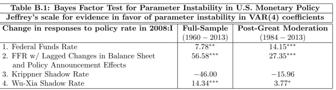
The …rst line of Table B.1 shows

_B

for the model comparison using the e¤ective FFR as the

monetary instrument for the entire post-war sample (1960:I-2013:III) and for the post-Great

Moderation sample (1984:I-2013:III). We …nd strong evidence against the model with constant

parameters using each of the two sub-samples, respectively. The results favor the model with

parameter instability over the baseline model, thus suggesting some added explanatory value

by allowing the parameters to change when the economy encounters the ZLB.

2.3

Monetary Policy at the ZLB

Ideally, we want to be able to account for the e¤ects of the Fed’s unconventional policy action

during the times in which the FFR does not ‡uctuate. Using the FFR alone to represent policy

would suggest that the Fed was inactive during the depths of the …nancial crisis and did little

to stimulate the recovery. Therefore, we need a way to incorporate the policy accommodation

associated with the balance sheet liquidity programs and the use of forward guidance. In the

next section, we augment the VAR with announcement e¤ects and the Fed’s balance sheet to

determine whether accounting for alternative policy instruments are su¢ cient to preserve the

dynamic responses suggested by the benchmark VAR model. Finally, we estimate a shadow

rate and use this as a proxy for the policy instrument during the ZLB period.

2.3.1

Adding Alternative Monetary Instruments

As we mentioned above, during the ZLB period, the Federal Reserve began to utilize alternative

policy measures. These measures were intended to provide temporary injections of liquidity and

often targeted yields for longer maturity assets. These policies also represented a substantial

policies is include them directly in the VAR by using dummy variables.

Augmenting the standard VAR model to account for the use of these instruments is not

straightforward. The policies are often thought to have both implementation e¤ects and

an-nouncement e¤ects— that is, the stance of policy could be thought to change both at the times

the programs were announced and at the times the balance sheet actually changed.

One way

to add these instruments into the model is to include event dummies for announcements and

to include changes in the size of the Fed’s balance sheet. Let

B

represent the di¤erence in the

size of the Fed’s balance sheet from

t

1

to

t

and let

P

be a dummy variable that indicates

the announcement of a future Fed action. Then, the VAR becomes

2

6

4

X

R

3

7

5

=

2

6

4

A

X

₍

_L

₎

_A

₍

_L

₎

A

(

L

)

A

(

L

)

3

7

5

2

6

4

X

R

3

7

5

+

2

6

4

A

BX

₍

_L

₎

_A

₍

_L

₎

0

0

3

7

5

2

6

4

B

P

3

7

5

+

2

6

4

"

"

3

7

5

;

where the zero restrictions impose orthogonality between the unconventional policies and the

e¤ective funds rate.

We can then determine whether accounting for alternative policy instruments is su¢ cient to

preserve the structure of the VAR into the ZLB period: Does including

A

(

L

)

and

A

(

L

)

make the VAR consistent across the ZLB period? The second line of Table B.1 shows the

results of the Bayes Factor comparing VAR’s with exogenous controls for

B

and

P

in the

equations for

X

, with and without parameter instability at the ZLB. The evidence against

the model with constant parameters is even stronger than when using only the FFR, as in the

previous section. The additional

B

and

P

terms come into play primarily around the early

stages of the …nancial crisis and over the period witnessing drastic cuts in the FFR towards

the ZLB. Incorporating these additional dynamics emphasizes the variation underlying the

structural form of the model and ampli…es the importance of allowing for parameter instability.

This very strong evidence favoring changing coe¢ cients over constant coe¢ cients suggests

that accounting for the unconventional policy via event dummies is not su¢ cient to maintain

linearity.

Figure B.1 compares the impulse responses to a shock to the FFR in the benchmark to the

VAR that includes

B

and

P

. As in the previous analysis, the right-hand column shows the

median point estimate and 68-percent posterior coverage intervals for the impulse responses

estimated using the full-sample VAR, with

B

and

P

. The dark blue lines and blue shaded

regions replicate the benchmark results. The median point estimates of the full-sample seem

to deviate only slightly from the benchmark, with a more signi…cant change for the response

of commodity prices, but the posterior coverage is considerably wider. Introducing additional

structure into the model and requiring estimation of the coe¢ cients on

B

and

P

degrade the

precision with which the rest of the model parameters are estimated.

Similar to the results above, accounting for the FFR, the balance sheet, and signi…cant

policy events produces a su¢ cient representative of policy for the full post-war period, including

a majority of non-ZLB data. However, augmenting the model in this way may be an ine¢ cient

approach for future empirical work once the policy environment returns to a normal,

non-ZLB environment and these unconventional policies are no longer in use. The Fed has a

variety of alternative policy programs in its arsenal but does not need to use them when it can

adjust the FFR e¤ectively. Including

B

and

P

introduces more parameters to estimate and

more structure in the model, especially if imposing identifying restrictions in terms of their

relationships with the other variables in the model. In response to this, we pose the question:

can we …nd a proxy measurement of

R

that captures the stance of policy across all periods?

We attempt to answer this question in the remainder of the paper.

2.3.2

Shadow Short Rates

One of the Fed’s stated objectives in conducting unconventional monetary policy was to a¤ect

interest rates for longer maturity assets, suggesting that examining the term structure of

interest rates could uncover a potential alternative policy instrument. Because the nominal

short rate is constrained during the ZLB period, Black (1995) proposed a model with a …ctitious

shadow bond with the same maturity as the policy instrument and an unconstrained shadow

shadow short rate,

r

, and zero:

R

= max

f

r

;

0

g

:

(2.3)

When the nominal rate binds at the ZLB, the shadow rate is unconstrained and can fall below

zero. Krippner (2012), Wu & Xia (2014), and Christensen & Rudebusch (2013) estimate

versions of this shadow rate using …nancial market data spanning the full term structure.

Krippner (2012) modi…es the Black (1995) framework of modeling interest rates as options by

calculating the value of a call option to hold cash. This methodology includes two latent factors

with a series of restrictive normalizations in order to apply the option-pricing framework.

Krippner (2012) uses numerical integration to generate closed-form solutions for bond prices

and yields within the shadow term structure. Christensen & Rudebusch (2013) apply the

option-based pricing approach formalized by Krippner (2012) to estimate the …rst three-factor

shadow rate model using data on Japanese government bond yields. Alternatively, Wu & Xia

(2013) construct an analytical approximation of forward rates in discrete time. This allows

for a more straightforward estimation approach than the other shadow rate methodologies.

The authors include three latent factors and apply the normalization technique introduced by

Joslin et al. (2011).

Krippner (2012) and Wu & Xia (2014) argue that the shadow rate can be used to measure

the stance of monetary policy when nominal rates hit the ZLB. The shadow rate, however, is a

purely …nancial construct that does not take into account its e¤ects on macro variables. If we

are to use the shadow rate in empirical models of monetary policy, we need to know whether

standard VAR models can be extended through the ZLB period by replacing the e¤ective FFR

with the exogenously constructed shadow rate or if the ZLB period, in and of itself, requires

an alternative model.

Following the methodology of Krippner (2012), we construct the shadow rate use data on

the full yield curve, out to the 30-year Treasury bond. The dataset spans 1986:IV through

2013:III so, in principle, we can derive a shadow rate for this entire period. However, we will

only need the shadow rate values to proxy for the FFR once hitting the ZLB. The details

method generates a monthly shadow rate. However, in order to use this as the policy

instru-ment in the VAR(4) analysis, we aggregate over the quarter by averaging the estimated values

for the shadow rate over each quarter. The shadow rate developed in Wu & Xia (2014) is

made publicly available on Federal Reserve Bank of Atlanta website. We convert the monthly

frequency to a quarterly frequency in the same way as with our version of Krippner’s shadow

rate.

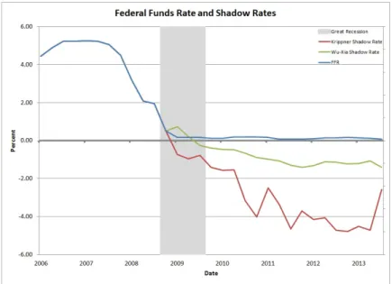
Figure B.3 shows a sub-sample from 2006:I-2013:III of the quarterly policy instruments

used for estimation in the VAR. Prior to 2009:I, all policy instruments use observed values of

the nominal FFR. From 2009:I through the end of the sample, we substitute the two shadow

rate measures for the e¤ective fed funds rate in separate VAR’s. By construction, when the

nominal FFR is su¢ ciently far from zero, it and the shadow rate move consistently together.

The shadow rate should be equal to the nominal short rate when the nominal short rate is

positive and the model preserves this relationship up to a small measurement error. However,

once the FFR e¤ectively reaches the ZLB in 2008:IV, the shadow rate becomes increasingly

more negative as the Fed took action to jump-start the economy.

Therefore, as a third alternative treatment option for the ZLB period, we estimate the

same VAR(4) as above with this new hybrid policy measurement. Lines 3 and 4 of Table 1

show results of the Bayes Factor model comparisons using both the Krippner (2012) and Wu

& Xia (2014) shadow rates as the policy instrument, respectively. Similar to the case with

using the FFR, the linear VAR using the Wu & Xia (2014) shadow rate still favors the model

incorporating parameter instability around 2008:I, after the onset of the …nancial crisis. There

is very strong evidence in favor of the model allowing for a shift in the macro responses over the

entire post-war sample. The evidence is still positive, but much less strong for the post-Great

Moderation subsample. Conversely, when using the Krippner (2012) shadow rate, the results

favor the constant parameter model for both the full post-war or the post-Great Moderation

samples. This shadow rate exhibits much richer dynamics over the crisis and ZLB periods,

taking on greater negative values. It appears that this variation, in contrast to the FFR or

the smoother path of the Wu & Xia (2014) shadow rate, allows the Krippner (2012) shadow

These results elicit the question: is the shadow rate a su¢ cient proxy for the stance of policy

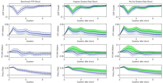
to preserve the linearity in the monetary models? Figure B.4 shows the impulse responses of

the VAR using the shadow rates substituted for the e¤ective funds rate at the ZLB. The

…rst column repeats the benchmark using the FFR from 1960:1-2007:IV from Figure B.1.

The center column estimates the VAR with the Krippner (2012) shadow rate as the policy

instrument from 2009:I-2013:III and the right column estimates the VAR with the Wu &

Xia (2014) shadow rate as the policy instrument. Using either shadow rate to represent policy

generates posterior coverages for the responses of all macro variables similar to the benchmark.

The median benchmark responses fall within the posterior coverage for the full-sample analyses

in all cases except for a small bias on the persistence of the policy shock’s e¤ect on the policy

rate itself. Again, the ZLB period itself is very short compared to the entire sample and the

lack of signi…cant di¤erences in responses may be due to the stronger in‡uence of pre-ZLB data.

Even with the subtle di¤erences noted here, the shadow rates seem to preserve the qualitative

(and much of the quantitative) relationships between our macroeconomic indicators and the

e¤ects of monetary policy actions.

We are interested in whether the shadow rate provides a su¢ cient proxy for monetary policy

in the ZLB environment, in particular to explain the e¤ects of policy throughout the economic

contraction of the recent recession. The objective is to use the shadow rate to represent the

signi…cant policy stimulus associated with unconventional policies when the FFR does not

deviate from the ZLB. The substantial downward movement of the shadow rate occurs in the

early stages of the Great Recession, with increasingly negative shadow rates while the FFR is

near zero.

Wu & Xia (2014) treat this period di¤erently than the subsequent ZLB period once the

economy is no longer in recession but the FFR is still near zero and unconventional policies

are still in use. They argue for using the shadow rate to model policy action only after the

recessionary conditions subside. We would like to construct a comprehensive measure of policy

even during the recessionary period. The large negative shocks that pushed the economy into

recession and drove the FFR towards zero are important for determining the validity of the

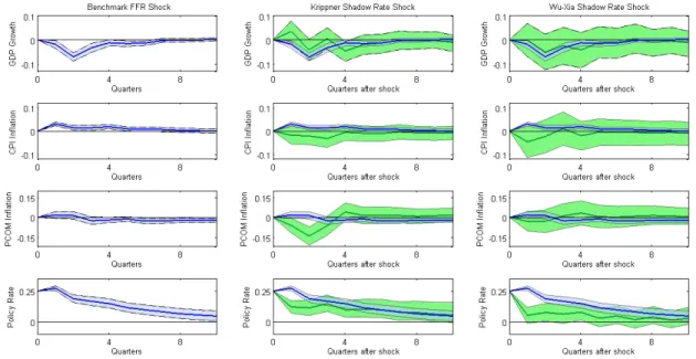
We re-estimate the VAR and include only the period after the onset of the ZLB to look

speci…cally at economic conditions when the shadow rate should provide more information

than the FFR alone.

_{Figure B.5 shows the impulse responses of the benchmark VAR(4)}

and then using the shadow rates over the period from 2008:I through 2013:III, isolating the

period during which we model the ZLB as binding. During this time the nominal FFR hardly

‡uctuated from zero and thus could not e¤ect much change itself on the overall economy. The

shadow rates incorporate other external in‡uences on both current policy as well as market

expectations of future policy and future economic conditions. Thus, the responses of macro

aggregates to shocks to this alternative policy measurement illustrate more comprehensive

policy action during the severe economic contraction.

The impulse responses are estimated with much less precision and the posterior coverage

is considerably wider for the VAR shadow rate estimation using only ZLB data than for the

benchmark. As a result, the median benchmark responses tend to fall within the considerably

wide posterior coverage. The median point estimate of the response of output is comparable

when examining the benchmark and using the Wu-Xia shadow rate over the ZLB period. The

Krippner shadow rate does not induce a contractionary response until after one period but then

moves in a similar fashion to the benchmark. Not surprisingly, the median responses of in‡ation

and commodity prices still ‡uctuate from the benchmark. The response of in‡ation implies a

price puzzle in the benchmark but neither of the shadow rates replicate this type of response

during the ZLB period. Contractionary policy shocks are associated with falling in‡ation

using either shadow rate. As we previously discussed, the shadow rate may incorporate future

expectations as it extracts data from interest rates and investment decisions. Finally, while

the response of the policy rate to its own shocks dissipates more quickly with the shadow rates

than the benchmark, the qualitative nature of the response matches that of the FFR in normal

times.

1 1

Of course, given the data limitations for this period, error bands are expected to be large and results will be only suggestive.

1 2

2.3.3

Model Performance

Finally, we test whether there are appreciable di¤erences in the impulse responses to a shock

to the shadow short rate estimated over the full sample versus the responses to a shock to the

FFR in our benchmark pre-ZLB sample. In order to do this, we construct the Kullback-Leibler

Divergence (KLD) between the posterior distribution of the benchmark VAR parameters and

the posterior distribution of the VAR parameters estimated using the alternative policy

in-struments.

We can think of the KLD as a type of loss function that measures deviations

between distributions. We take the benchmark, pre-ZLB posterior parameter distributions as

the truth and measure the extent to which the posterior distributions di¤er from this when

using the shadow rate proxies. Ideally, we want to look at the di¤erence in the distributions of

the impulse responses themselves. However, since there is a one-to-one mapping between the

impulse responses functions and the VAR coe¢ cient and covariance matrices, we can use the

output of the Gibbs sampler to analyze the posterior distribution of the parameter estimates

directly.

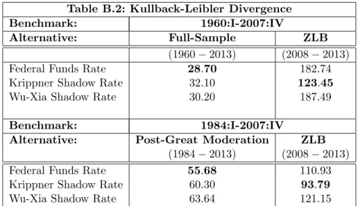
Table B.2 gives the values of the KLD between the post-war, pre-ZLB benchmark

(1960:I-2007:IV) and the full-sample (1960:I-2013:III) when using the FFR and each of the two shadow

rates. When including both the pre-ZLB and ZLB periods within the sample, the model

in which the FFR is used to represent policy the entire time produces the smallest KLD,

thus showing the smallest deviation from the benchmark. This is in agreement with our

previous results using the full-sample with a majority of non-ZLB data. However, when looking

speci…cally at the ZLB period, the posterior distribution of VAR parameters estimated with the

shadow rate of Krippner (2012) has the smallest KLD, thus exhibiting less variation than the

distributions using the FFR or the shadow rate of Wu & Xia (2014). The results are the same if

we adjust the benchmark to only consider data after the end of the Great Moderation, therefore

estimating the VAR using data from 1984:I-2007:IV to establish our basis for comparison.

responses using the FFR and the shadow rates.

Again, the KLD produced from the FFR is smaller than those of the other two models for

both the full, post-Great Moderation (1984:I-2013:III) sample. Furthermore, the KLD using

the Krippner (2012) shadow rate is smallest for the ZLB sub-sample. Removing the in‡uence

of pre-ZLB data in the dataset by excluding the …rst 24 years of data allows for the shadow rate

modi…cations at the ZLB to achieve greater success at merging a comprehensive, continuous

representation of policy between these two periods.

We cannot compute the impulse responses of macroeconomic variables to the FFR during

the ZLB period alone as the policy instrument did not exhibit meaningful variation over this

time. When at the ZLB, the shadow rate of Krippner (2012) more closely recovers some

of the benchmark macro dynamics of the pre-ZLB period and these are further preserved if

we employ a full dataset over the entire post-war period, including the years at the ZLB.

We have also found that controlling for the size of the Fed’s balance sheet and signi…cant

policy announcements regarding alternative policy programs allows for recovering our baseline

dynamics and provides options to researchers seeking to model economies in which the central

bank is constrained by the ZLB. Having these anomalous years of data between extended

episodes of normal economic activity does not seem to prohibit the use of standard VAR

analyses for the e¤ects of monetary policy.

2.3.4

The Bottom Line

The ZLB period poses an interesting dilemma for empirical researchers. At the outset, we

posed a series of questions for the future empirical study of monetary policy, assuming that

the FFR is the policy instrument when normalcy returns. First, how large are the biases in

the estimated IRF’s if one uses the FFR for the full sample? When estimating the linear VAR

model over a long time span, inclusive of a period at the ZLB, we …nd that it is su¢ cient to

simply use the FFR as the policy instrument. While the results will be slightly biased, the

biases appear to be small. Once the economy lifts-o¤ from the ZLB and returns to normal

conditions, this bias should be mitigated and the majority of non-ZLB data should dominate

the results.

biases? Representing the policy instrument with a combination of measurements of the FFR,

changes in the size of the Fed’s balance sheet, and indicator variables for signi…cant policy

events within the VAR over the full post-war period still produces similar, if not larger, biases

to those produced by the model using only the FFR. This exercise requires estimation of

additional parameters associated with policies unique to the ZLB environment and thus may

introduce ine¢ ciencies when using a dataset consisting of predominantly non-ZLB data.

Third, does exchanging either shadow short rate mitigate these biases? We …nd that should

one wish to substitute a shadow rate proxy for the policy instrument during the ZLB period,

hoping to maintain consistent model dynamics throughout the time series, one must recognize

that the shadow rate methodology does not achieve a consistent model in all circumstances.

The choice over which shadow rate to incorporate will dictate whether or not accounting for

structural change is required.

Finally, which shadow short rate does a better job at mitigating these biases? Interestingly,

should one attempt to examine particular ZLB periods in isolation, neither the FFR nor the

shadow rate serve as an adequate representation of policy and do not produce the expected

relationship between e¤ective monetary policy and macroeconomic ‡uctuations. Therefore,

modeling this unique period requires further adjustments and a linear model may not su¢ ce.

2.4

Conclusions

Researchers attempting to measure the e¤ects of monetary policy during the …nancial crisis

and subsequent recession beginning in 2008 have encountered di¢ culties when trying to use

the FFR which essentially ‡atlines at zero for much of the period under consideration. We

have proposed using the shadow rate as a measurement of policy which is able to ‡uctuate to

negative values when the e¤ective central bank policy rate faces a binding constraint at zero.

Our results suggest that the shadow rate acts as a good proxy for monetary policy throughout

the ZLB environment only if using a dataset that spans the pre-ZLB period throughout the

ZLB environment. However, the shadow rate is and insu¢ cient proxy for a comprehensive

measurement of monetary policy when examining the ZLB period in isolation.

the monetary authority has indeed been successful at implementing expansionary policy albeit

through alternative mechanisms. An important point to note is that the economy has witnessed

a break in the instrument used to enact policy but not a break in the e¤ects of monetary

policy on the macroeconomy. Economic researchers use the FFR as a measurement of the

policy instrument for the post-WWII era even though the Fed targeted non-borrowed reserves

from 1979-1982 and borrowed reserves from late 1982 through the mid-1980’s. It did not stop

targeting M1 until 1987 and M2 until 1993 and began announcing formal targets for the FFR

only in 1994. Similarly to that change in the behavior of central bankers, the ZLB period

beginning in December 2008 has rendered the traditional policy tool impotent for stimulating

economic activity. The Fed has successfully utilized balance sheet items as instruments and

introduced a much more expansive period of alternative policy measures than the time spent

targeting non-borrowed/borrowed reserves. In order to accurately represent monetary policy

CHAPTER 3 MONETARY POLICY AND MACRO FACTORS AT THE ZLB

3.1

Introduction

The impaired functioning of …nancial markets, leading to the …nancial crisis and recession of

2008 and 2009, triggered substantial policy action in major economies around the world. For

the …rst time since the Great Depression, U.S. interest rates faced the binding constraint of

the zero lower bound (ZLB), sti‡ing the e¢ cacy of e¤orts of the Federal Reserve to stimulate

economic activity using its standard policy instrument. This forced the adoption of alternative

monetary policy instruments to combat the recession. The Fed broadened its lender-of-last

resort policies, implemented multiple rounds of quantitative easing and used carefully selected

language as forward guidance in its FOMC statements to steer market expectations.

The FOMC policy rate has been pegged e¤ectively at zero since December 2008.

Short-term nominal interest rates have traditionally been considered an indicator of the stance of

monetary policy - looser policy coincides with lower interest rates. However, when interest rates

face a binding constraint at zero, the true policy stance becomes obscured. Tallman & Zaman

(2012) highlight that most Taylor-type rules for monetary policy would have recommended a

negative policy rate starting in 2009 through 2012. This suggests that since the nominal FFR

could not fall below zero, policymakers faced substantial constraints regarding the deviation of

the desired path of the policy rate from that which was feasible. Bernanke & Reinhart (2004)

discuss various strategies for stimulating an economy facing the ZLB. In order to mitigate

this restriction, the Fed began targeting lower long-term interest rates through purchases of

longer-term securities with quantitative easing (QE1 and QE2) and the Maturities Extension

Program (Operation Twist).

Such unconventional policy measures can ease the perceived

1