NUCLEAR REACTION RATE UNCERTAINTIES AND THE22Ne(p, )23Na REACTION:
CLASSICAL NOVAE AND GLOBULAR CLUSTERS
Keegan John Kelly
A dissertation submitted to the faculty at the University of North Carolina at Chapel Hill in partial fulfillment of the requirements for the degree of Doctor of Philosophy in the Department of Physics.
Chapel Hill 2016
Approved by:
ABSTRACT
Keegan John Kelly: Nuclear Reaction Rate Uncertainties and the22Ne(p, )23Na Reaction:
Classical Novae and Globular Clusters (Under the direction of Arthur E. Champagne)
The overall theme of this thesis is the advancement of nuclear astrophysics via the analysis of stellar processes in the presence of varying levels of precision in the available nuclear data. With regard to classical novae, the level of mixing that occurs between the outer layers of the white dwarf core and the solar accreted material in oxygen-neon novae is presently undetermined by stellar models, but the nuclear data relevant to these explosive phenomena are fairly precise. This precision allowed for the identification of a series of elemental ratios indicative of the level of mixing occurring in novae. Direct comparisons of the modelled elemental ratios to observations showed that there is likely to be much less of this mixing than was previously assumed. Thus, our understanding of classical novae was altered via the investigation of the nuclear reactions relevant to this phenomenon.
However, this level of experimental precision is rare and large nuclear reaction uncertainties can hinder our understanding of certain astrophysical phenomena. For example, it is commonly believed that uncertainties in the 22Ne(p, )23Na reaction rate at temperatures relevant to thermally-pulsing asymptotic giant branch
stars are largely responsible for our inability to explain the observed sodium-oxygen anti-correlation in globular clusters. With this motivation, resonances in the 22Ne(p, )23Na reaction at Ec.m.
r = 458, 417, 178, and 151 keV were measured. The direct-capture contribution was also measured at Elab
p = 425 keV. It was determined that the 22Ne(p, )23Na reaction rate in the astrophysically relevant temperature range
ACKNOWLEDGEMENTS
Nobody makes it through life without copious amounts of assistance from other people along the way. Everyone needs to be taught, directed, advised, and pushed to get to where they need to be in life. The exact location of “where they need to be” may not be immediately clear, which makes preparation pretty challenging. Instead, my experience has shown me that the best thing to do is just learn what you can from who you can as you slowly work your way towards where you need to be.
My physics career really started back in high school. I knew for a while that I wanted to get into science, but you couldn’t take physics until senior year in my high school. I took Earth science, biology, and chemistry, in that order, and felt that I was getting closer to something that I could spend my life doing, but I wasn’t quite there yet. Then physics hit senior year and the light bulb turned on. My physics teacher in high school, Dr. Barry Glickstein, really encouraged my interest in physics by giving me Richard Feynman books to read outside of class. That experience solidified my choice to study physics, so I’d like to thank Dr. Glickstein for helping start my physics career.
After high school I did my undergrad at SUNY Geneseo. The physics professors at Geneseo were all extremely intelligent, excited about physics, and excellent teachers. It was a great environment for the next step in my physics career. I’d like to thank all of the SUNY Geneseo physics professors because I acquired my entire physics knowledge base from them, but I owe a great deal more to Dr. Kurt Fletcher. Kurt o↵ered me my first summer research position and taught me the basics of how to do research. I think that he took a little bit of a chance on me, but that experience paved the way for the next stages of my life. I don’t think that it is any coincidence that I chose UNC for my graduate career considering Kurt is also a UNC/TUNL alum.
convinced that I really understand anything at all!). Thanks for pushing me to understand the physics, Tom.
I shared an office with Dr. Johnny Cesaratto during my first summer at LENA. Johnny was a wealth of knowledge about every detail of LENA and was always enthusiastically willing to share what he could with me about LENA, so I’d like to thank him for that. It was more than a little intimidating to be sitting at my desk during my first summer struggling to understand the physics of various aspects of LENA, only to have Tom burst into office and launch into a conversation with Johnny that was miles beyond what I was prepared to discuss at the time. It’s strange looking back at those conversations now knowing that, in theory, I am about as far into graduate school as he was at then. At this point I think that I could hold my own in conversations like those, but the shock of hearing just how much I had to learn is still fresh in my mind.
I officially joined LENA during my first year when Dr. Art Champagne accepted me as a graduate student. Later in my graduate career I would closely with Art during my Ph.D project, but I primarily worked with Dr. Christian Iliadis during my Master’s project. Toward the end of my first year I sat down with both Art and Christian with the intent of deciding on my first project. At the time I was positive that I wanted to be more on the theoretical side of physics. Despite their best e↵orts to sway me towards experimental physics, I stood my ground and began working on my Master’s project, a calculational project dealing with classical novae. Even though Art was my official advisor, Christian took time out of his schedule to help guide and direct my project whenever I needed it. I learned careful and complete research practice from Christian, but I’d especially like to thank Christian for helping me to, “See the forest for the trees”, as he’d say.
My Master’s project would have been 10x as difficult if it weren’t for the assistance of Lori Downen. Lori was in the process of completing a project similar to my Master’s project just as I was starting out and I’m forever indebted to her for imparting as much of her knowledge as I could handle about the nucleosynthesis network code at LENA and about the UNC ion implanter as well. Whether they realize it or not, everyone at LENA is also indebted to Lori being the only one willing to regularly supply soap and clean towels to the LENA control room (Thank you!). Lori and I became a team for many aspects of LENA. We ran experiments, etched target backings, and set up data-acquisition electronics together among a host of other tasks that I’m probably forgetting to mention. It is an enormous testament to her great personality and teamwork skills that we were able to work so well together for this many years.
all about the lab through the “espresso-fuelled accelerator shifts” [Daigle,2013] we ran for his experiment set the tone for my graduate school career, and that’s why I’d like to thank Stephen. Becoming an operator during Stephen’s experiment a↵orded me the privilege to work on the experiment of Dr. Chris Howard along with Dr. Anne Sallaska. I consider myself lucky to have worked with the legendary Dr. Bob Runkle during this process as well (your $20 will be forever immortalized in the ECR log book, Bob). Everyone involved in this experiment had such a great attitude about experimental physics. It was during this experiment that I finally decided that I wanted to pursue an experimental project myself, and so I thank everyone involved in Chris’ experiment for that.
I’ve never met anyone as methodical and thorough as Dr. Matt Buckner. It takes a special kind of person to run two experiments at LENA, run into as many accelerator and lab-related problems as he did, and still possess the character and motivation to not cut any corners. I was already in the habit of taking a lot of notes before Matt, Lori, and I worked together on setting up the NaI annulus and data-acquisition electronics for Matt’s second experiment, but the usefulness and level of detail in his note taking showed me just how important it was to take notes on everything possible. Matt sat with me for hours during his Ph.D experiment letting me (poorly) operate the ECR ion source even though he could easily do a much better job than me and also taught me a great deal about the LENAGeantsimulation. Matt significantly impacted almost every part of my path through research at LENA and I owe him a sincere thank you for that.
Shortly after helping with Stephen’s and Chris’ experiments I walked into Art’s office and said that I’d like to have an experimental measurement for my Ph.D project instead of a theory/modelling-based project. Without even blinking, Art just said, “We can do that”, as if it had been part of the plan the entire time. The level of patience that Art has as an advisor is difficult to comprehend. He allowed me the freedom to pursue any research avenue that I had the motivation to follow, which allowed me to feel true ownership over my project. Not surprisingly, this freedom caused me to take some wrong turns every now and again, but I think that’s when I really learned something. Even looking back now at all of our meetings about my work I honestly can’t tell if we were just making up the path as we went through my Ph.D project or if Art actually had everything planned out in advance and was just waiting for me to get there. Either way, Art’s advisement clearly puts the ball in the student’s court. This requires patience and trust in the student that I don’t believe any incoming graduate student would (or should) think themselves worthy of. I now understand the importance of this kind of advisement and I cannot thank Art enough for advising me through my graduate career.
established before I joined the group, so I was very excited to see him rejoin LENA as a postdoc a few years after first leaving LENA. I, along with the entirety of LENA, owe Richard a gracious thank you for establishing some of the most heavily-used computer codes at LENA. Now a faculty member at NC State and LENA/TUNL faculty member as well, I’m looking forward to seeing the future of LENA unfold with Richard in a more prominent role.
At this point I would like to thank my Ph.D committee members that have not yet been acknowledged, Dr. Fabian Heitsch and Dr. Nick Law. Thank you both for agreeing to appear on my committee and for providing helpful feedback during and after my prelim and thesis defense. I’d like to thank Fabian for also appearing on my Master’s committee. Fabian has been a part of every one of my graduate school milestones and I sincerely appreciate that.
Moving on to the future of LENA, Jack Dermigny, Sean Hunt, and Andrew Cooper arrived at UNC one year after me and after my second year they had all joined LENA. There are a number of ways that having this number of students in the same year could have gone wrong in terms of project and expertise overlap, but these three have made it work to perfection. Between Jack, Andrew, and Sean, LENA has an expert in data analysis, accelerator development and upkeep, and detector characterization and DAQ electronics. I can only hope that they’ve learned half as much from me as I’ve learned from them. David Little joined LENA a couple of years after Jack, Sean, and Andrew. His tenacious questioning of what he hasn’t learned yet has allowed him to understand details about certain aspects of LENA that I never even thought to ask. I have faith that David will one day master the entire laboratory, inside and out.
No discussion of LENA is complete without mention of the LENA/TUNL technical sta↵members John Dunham, Richard O’Quinn, Bret Carlin, Chris Westerfeldt, and Brian Walsh. LENA prides itself on being a student-run laboratory. The students develop the materials with which to run their own experiments, they take their own data, and they do what they can to fix what needs to be fixed around the lab, but when somethingreally breaks, then it’s time to call in the tech sta↵. Each of these TUNL employees were instrumental in allowing LENA to continuously make progress in one way or another. I am extremely grateful for their expertise and their assistance in getting through the countless issues that arose during every-day operation of LENA.
Thank you for pushing me to apply for jobs when I wanted to write my thesis instead, for having faith in my ability to find us a job after graduate school even though you could have easily gotten one yourself, and most importantly, for loving me through this whole process of graduate school. I love you and I can’t wait to see what happens next in our lives together.
Finally, I’d like to thank my parents and my brothers. There was a time during my undergraduate career that I thought that I was not interested in graduate school because I would come out on the other side of it at least 27 years old and still without a real job. I said this to my mom as we drove to the mall sometime in the middle of my undergraduate career. The look I got back from her could have started a fire if I wasn’t there to intercept it. She made me immediately realize how immature that viewpoint was because I would be squandering a fantastic opportunity to learn so much more than I thought was possible and I might not get that opportunity back. My mom, dad, and brothers were always encouraging of my choices to do what I wanted to do and go where I wanted to go, as long as I tried my hardest along the way. Looking back, I think that there was an undertone to that encouragement that was telling me to try my hardest, but also to not go too far from home away in the end. As my fianc´ee and I prepare to move to a completely di↵erent part of the country, I think that I picked up on that last part a little bit too late. Even though I’m miles and miles away from home and I can’t come back for all of the family get togethers, I’m never going to forget where I came from. I know that family is more important than anything else because you that’s what you’ve taught me. So, I’m dedicating my entire thesis to my mom, my dad, and my brothers. Thank you all for making me who I am today.
TABLE OF CONTENTS
LIST OF TABLES . . . xv
LIST OF FIGURES . . . xvi
LIST OF ABBREVIATIONS AND SYMBOLS . . . xix
1 A GENERAL INTRODUCTION . . . 1
1.1 Introduction . . . 1
1.2 Phases of Stellar Evolution . . . 2
1.3 Nuclear Physics Basics . . . 6
1.3.1 Definition of the Cross Section . . . 6
1.3.2 Transmission Through the Coulomb Barrier . . . 7
1.3.3 Nuclear Reaction Resonances . . . 9
1.4 Nuclear Physics in Stellar Environments . . . 11
1.4.1 Narrow-Resonance Reaction Rates . . . 12
1.4.2 Direct-Capture Reaction Rates . . . 13
1.5 The Underlying Theme . . . 15
2 NUCLEAR MIXING METERS FOR CLASSICAL NOVAE. . . 19
2.1 Preface . . . 19
2.2 Introduction and Background on Classical Novae . . . 19
2.3 Hydrodynamic Simulations . . . 22
2.4 Monte Carlo Post-Processing Nucleosynthesis Calculations of Classical Novae . . . 28
2.5 Identification Methods of Important Reactions to Measure . . . 31
2.6 Comparison to Observations . . . 36
2.8 Conclusions Regarding Nuclear Mixing Meters for ONe Classical Novae . . . 39
3 THE GLOBULAR CLUSTER Na-O ANTI-CORRELATION . . . 43
3.1 Preface . . . 43
3.2 Globular Cluster Background . . . 44
3.3 AGB Stellar Evolution . . . 48
3.4 Monte Carlo Post-Processing Nucleosynthesis Calculations of a 5 TP-AGB Star . . . 51
3.5 Determination of the Important Processes to Measure in22Ne(p, )23Na . . . . 53
4 ACCELERATORS AND DETECTORS . . . 60
4.1 LENA: The Laboratory for Experimental Nuclear Astrophysics . . . 60
4.2 JN van de Graa↵Accelerator . . . 61
4.3 Electron Cyclotron Resonance Ion Source . . . 64
4.3.1 Basics of Operation . . . 64
4.3.2 ECR Acceleration Column Upgrade . . . 67
4.3.3 ECR Beam Pulsing . . . 68
4.4 Detectors . . . 73
5 TARGET FABRICATION AND CHARACTERIZATION . . . 78
5.1 Target Fabrication . . . 78
5.2 Rutherford Backscattering Spectrometry Measurements . . . 80
5.2.1 Motivation for RBS Measurements . . . 80
5.2.2 Experimental Details . . . 80
5.2.3 Analysis and Results of RBS Measurements . . . 84
5.3 Treatment of Target Degradation . . . 88
6 NEW RECOMMENDED ! (458 keV) FOR THE 22Ne(p, )23Na REACTION . . . . . 93
6.1 Motivation for Improved Data on the 458-keV Resonance . . . 93
6.2 Experimental Procedure . . . 94
6.4 Results . . . 100
6.5 Validation of the Technique and Comparison with Previous Results . . . 104
6.5.1 Experimental Yield Calculations . . . 104
6.5.2 Coincidence-Summing Corrections . . . 105
6.5.3 Results . . . 107
6.6 Conclusions . . . 108
7 LOW-ENERGY22Ne(p, )23Na MEASUREMENTS . . . . 111
7.1 Preface . . . 111
7.2 Resonance at Ec.m. r = 458 keV . . . 111
7.2.1 Coincidence Measurement of the 458-keV Resonance . . . 111
7.2.2 Maximum-Yield Measurement of the 458-keV Resonance . . . 113
7.2.3 Relative Measurement Method . . . 113
7.3 Resonance at Ec.m.r = 417 keV . . . 114
7.4 Direct-Capture Measurement at Elab p = 425 keV . . . 119
7.5 Data Analysis via a Markov-Chain Monte CarloTFractionFitter Method . . . 128
7.6 Resonance at Ec.m. r = 178 keV . . . 130
7.7 Resonance at Ec.m. r = 151 keV . . . 138
7.8 Thermonuclear Reaction Rate of22Ne(p, )23Na . . . 146
7.9 Astrophysical Impact . . . 153
8 CONCLUSIONS . . . 158
APPENDIX A ANGULAR CORRELATION THEORY . . . 161
APPENDIX B Geant4 COINCIDENCE-SUMMING CORRECTION CODE . . . 169
APPENDIX C COINCIDENCE-SUMMING CORRECTION METHOD VALIDATION 188
APPENDIX E INPUT FILE FORRatesMC . . . 193
LIST OF TABLES
2.1 Characteristics of the hydrodynamic classical nova models used in Chapter 2 . . . 23
2.2 Initial abundances for hydrodynamic classical nova models . . . 25
6.1 Branching ratios from the 458-keV resonance in the22Ne(p, )23Na reaction . . . 101
6.2 Summary of resonance strengths for the 458-keV resonance in22Ne(p, )23Na . . . 104
7.1 Singles and coincidence branching ratios from the 458-keV resonance in22Ne(p, )23Na . . . . 112
7.2 Singles and coincidence branching ratios from the 417-keV resonance in22Ne(p, )23Na . . . . 118
7.3 Singles and coincidence branching ratios from the 178-keV resonance in22Ne(p, )23Na . . . . 135
7.4 Tentative branching ratios from the 151-keV resonance in22Ne(p, )23Na . . . 142
7.5 Summary of resonance strengths and direct-capture cross sections for22Ne(p, )23Na . . . 148
LIST OF FIGURES
1.1 Hertzsprung-Russell diagram of globular cluster M5 fromSandquist et al.[1996] . . . 3
1.2 Image depicting the pp chains . . . 4
1.3 Image depicting the CNO cycles . . . 4
1.4 Image depicting the NeNa and MgAl cycles . . . 5
1.5 Plot of a fictional Breit-Wigner cross section . . . 10
1.6 Plot of the total cross section for the16O(p, )17F reaction fromIliadis[2015] . . . . 14
1.7 The Gamow peak for a stellar temperature of 0.1 GK . . . 16
2.1 Schematic representation of the binary classical nova scenario . . . 20
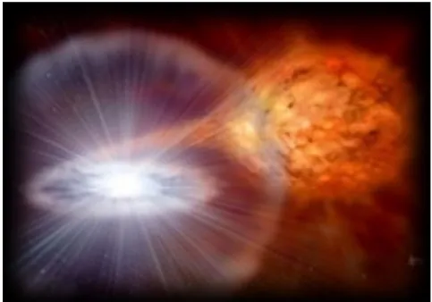
2.2 Artist’s rendition of a classical nova explosion . . . 20
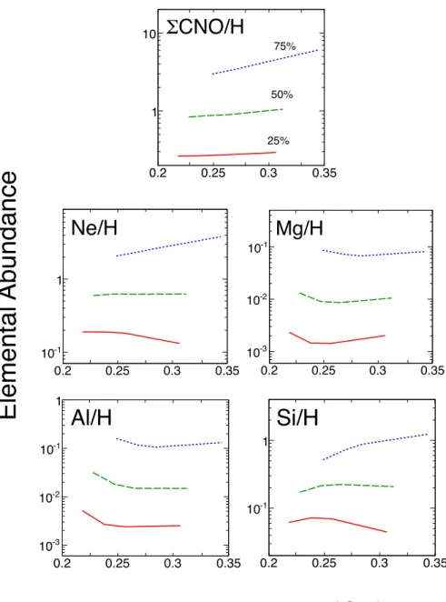
2.3 Initial results for nuclear mixing meters . . . 26
2.4 Single-plot representation of nuclear mixing meters . . . 27
2.5 Illustration of the instant-mixing approximation . . . 29
2.6 Illustration of the no-mixing approximation . . . 29
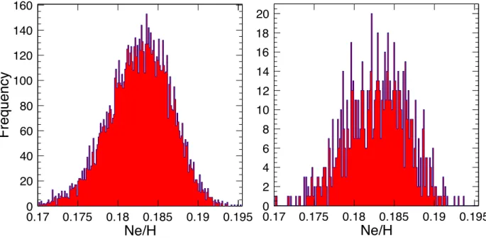
2.7 Comparison of Ne/H calculated with 1000 and 10000 Monte-Carlo calculations . . . 32
2.8 Ne/H ratio for a classical nova model with 25% mixing and a 1.30 M white dwarf . . . 33
2.9 The Si/H ratio for a classical nova model with 75% mixing a 1.35 M white dwarf . . . 34
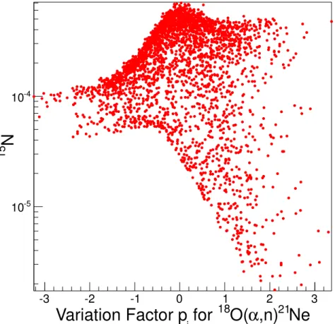
2.10 Correlation of the15N abundance to the18O(↵,n)21Ne rate variation factor . . . 35
2.11 Comparison of nuclear mixing meters to eight observed classical novae . . . 38
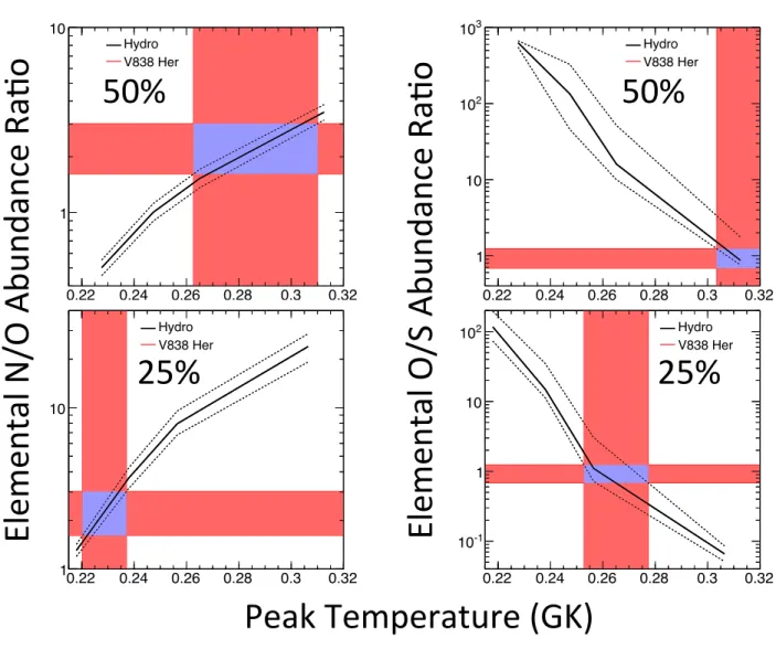
2.12 Comparison of N/O and O/S ratios assuming 50% and 25% mixing in classical novae . . . 40
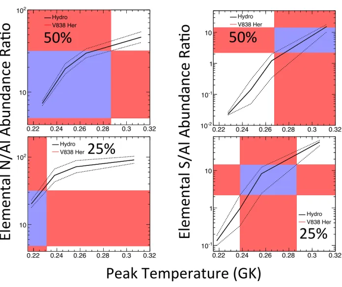
2.13 Comparison of N/Al and S/Al ratios assuming 50% and 25% mixing in classical novae . . . . 41
3.1 Triple main sequence observed in globular cluster NGC 2808 . . . 45
3.2 Na-O anti-correlation observed in globular cluster NGC 2808 . . . 46
3.3 Stellar structure of an AGB star before thermal pulses . . . 49
3.4 Onset of thermal pulses in a massive AGB star . . . 50
3.5 Temperature profile of a 5 M TP-AGB star . . . 50
3.6 The hot bottom burning process in TP-AGB stars . . . 52
3.7 Important reaction rates for production and destruction of23Na in TP-AGB stars . . . . 54
3.8 Illustration of the Monte Carlo reaction rate calculation procedure . . . 55
3.9 Reaction rate contribution plot for the22Ne(p, )23Na reaction rate . . . . 57
4.1 Top-down view of the Laboratory for Experimental Nuclear Astrophysics . . . 61
4.2 Side-view image of the target chamber at LENA fromCesaratto et al. [2010] . . . 62
4.3 Hydrogen plasma in the JN plasma bottle . . . 63
4.4 Image of the ECR ion source . . . 65
4.5 Image of the ECR acceleration column prior to its upgrade . . . 66
4.6 Illustration of the source of X rays from the old ECR acceleration column . . . 67
4.7 Image of the ECR acceleration column after its upgrade . . . 69
4.8 Waveform of measured beam current on target . . . 71
4.9 Data taken on the 151-keV resonance in18O(p, )19F using DC and pulsed ECR beams . . . 72
4.10 The LENA -coincidence spectrometer . . . 74
4.11 An example 2D coincidence spectrum that demonstrates coincidence gating . . . 76
4.12 Full-energy peak efficiency trend of the LENA HPGe detector . . . 77
5.1 Schematic view of the Eaton 3204 Positive Ion Implanter at UNC–Chapel Hill . . . 79
5.2 Typical yield curve from22Ne targets used for on-resonance data . . . . 81
5.3 Typical yield curve from22Ne targets used for o↵-resonance data . . . . 82
5.4 Typical target degradation trend for the thick targets . . . 83
5.5 The target wheel used during RBS data acquisition . . . 85
5.6 Example RBS data spectrum from a thin22Ne target . . . . 86
5.7 Trend of RBS spectra obtained after 0, 6, 10, and 12 C of accumulated data . . . 89
6.1 Experimental peak Gaussian FWHM versus energy trend for the HPGe detector . . . 95
6.2 Schematic of the data analysis used in this thesis . . . 96
6.3 Result of the best fit to the data on the22Ne(p, )23Na resonance atEc.m. r = 458 keV . . . . 102
6.4 Evidence for a new a primary transition from the 458-keV resonance in22Ne(p, )23Na . . . . 103
6.5 Experimental yields for primary transitions from the 458-keV resonance in22Ne(p, )23Na . . 109
7.1 Singles spectrum of the 417-keV resonance in22Ne(p, )23Na . . . 116
7.2 Evidence for new multiple transitions from the 417-keV resonance in22Ne(p, )23Na . . . 117
7.3 Comparison of the present and previous! (417 keV) values . . . 118
7.4 Singles spectrum of the direct-capture22Ne(p, )23Na data . . . 121
7.5 Coincidence spectrum of the direct-capture22Ne(p, )23Na data . . . 122
7.6 Direct-capture coincidence spectrum with various coincidence gates . . . 123
7.8 Comparison of DC!7082, 7488, 8664, & 8830 cross sections to literature . . . 126
7.9 Comparison of the DC!0 cross section and S-factor to literature . . . 127
7.10 R!440, R!2076, 440!0, and 2076!440 signals from the 178-keV resonance . . . 131
7.11 Singles spectrum of the 178-keV resonance in22Ne(p, )23Na . . . 132
7.12 Coincidence spectrum of the 178-keV resonance in22Ne(p, )23Na . . . 133
7.13 Comparison of on- and o↵-resonance coincidence data for the 178-keV resonance . . . 134
7.14 Posterior distribution for the coincidence R!2982 transition from the 178-keV resonance . . 136
7.15 Posterior distribution for the coincidence R!0 transition from the 178-keV resonance . . . . 137
7.16 440!0 and R!3914 signals from the 151-keV resonance . . . 138
7.17 Comparison of on- and o↵-resonance coincidence data from the 151-keV resonance . . . 139
7.18 Coincidence spectrum of the 151-keV resonance in the22Ne(p, )23Na reaction . . . 140
7.19 Data from the 151-keV resonance with various coincidence gates . . . 141
7.20 Posterior distribution ofNdata R observed from the fit to the 151-keV resonance . . . 143
7.21 Trends of reduced 2 andNdata R versus number of templates included in the fit . . . 145
7.22 Diagram of23Na levels with primary branches from resonances investigated in this thesis . . 147
7.23 Comparison of rate contribution plots before and after measurements made here . . . 150
7.24 Alternate representation of the contribution22Ne(p, )23Na rate contribution plot . . . 151
7.25 Present rate contribution plot to that calculated with 2x the literature DC rate . . . 152
7.26 Ratio of theSTARLIB 22Ne(p, )23Na rate to the present rate with uncertainties . . . 154
7.27 Correlations of reactions to23Na in TP-AGB stars after the present measurements . . . 155
7.28 23Na abundance distribution after the measurements made for this thesis . . . 157
LIST OF ABBREVIATIONS AND SYMBOLS
AGB Asymptotic Giant Branch
CN Classical Nova
DC Direct Capture or Direct Current, depending on usage ECR Electron Cyclotron Resonance
FWHM Full Width at Half Maximum
GC Globular Cluster
HB Horizontal branch
HBB Hot Bottom Burning
H-R Hertzsprung-Russell
LENA Laboratory for Experimental Nuclear Astrophysics
M Solar Mass
MS Main sequence
P-AGB Post-asymptotic giant branch
PN Planetary Nebula
RBS Rutherford Backscattering Spectrometry
RGB Red giant branch
TO Main sequence turn-o↵point
TP-AGB Thermally-Pulsing Asymptotic Giant Branch
TUNL Triangle Universities Nuclear Laboratory
1: A GENERAL INTRODUCTION
1.1: Introduction
Stellar fusion, including big-bang nucleosynthesis, cosmic-ray spallation, and nuclear fusion within stars, is responsible for creating all nuclei in the universe heavier than helium. The energy released during nuclear fusion supports stars against gravitational collapse and creates a sustainable environment in which light nuclei are fused together into higher mass elements. These light nuclei are, in a sense, fuel used to keep stars alive. In the simplest and youngest stars, a nuclear fusion cycle referred to as the proton-proton (pp) chains is the mechanism through which hydrogen, the lightest element possible, is burned to form helium, the second lightest element, releasing a significant amount of energy in the process. The helium that is formed can be thought of as the ashes of hydrogen burning via the pp chains. In stars consisting of higher mass elements, hydrogen fuel can be burned through other nuclear fusion chains that, while they are qualitatively di↵erent, still accomplish the same goal of fusing hydrogen into helium. Some of these various hydrogen burning sequences will be discussed in the next section.
Following the reduction of the hydrogen abundance to a level that H-burning reactions can no longer balance the star in hydrostatic equilibrium, the stellar temperature and density increase until helium-fusion sequences converting three 4He nuclei to a single 12C and subsequently the 12C(↵, )16O reaction become
1.2: Phases of Stellar Evolution
Depending on the initial stellar mass, stars can live for billions of years continuously undergoing stellar fusion of progressively heavier and heavier elements until either no new material can be fused, leaving the star as a dim dwarf, or until the gravitational contraction of the star cannot be upheld by energy release from nuclear fusion any longer, resulting in a more dramatic and violent end stage for the star in the form of a stellar explosion. The long lifetime of stars, relative to our own, means that the vast majority of stars will appear static to the casual observer. Given this fact, how can we obtain definite proof that stars truly evolve from one stage of the stellar life cycle to the next and do not simply remain as the unchanging entities they appear to be?
To paraphrase and expand upon the analogy byKippenhahn[1983], the difficulties faced by an astronomer observing stars are analogous to those problems that would be faced by someone who observes countless humans at varying stages of life, from newborns to the elderly, over the course of a single day. There would be no way to observe a baby growing old, but one could plot trends such as, for example, human height versus intelligence level. Noting that this trend is continuous, the observer would determine that all humans are the same type of being, only di↵ering by their stage of life. Astronomers follow this exact same methodology, with some obvious di↵erences. Instead of humans, they track stars, and instead of plotting human height versus intelligence level, they plot stellar luminosity versus temperature.
A plot of these stellar observables is referred to as a Hertzsprung-Russell diagram, or H-R diagram. An example H-R diagram is shown in Figure 1.1 for a group of stars referred to as globular cluster M5. Note that temperature increases from right to left on the x-axis. H-R diagrams show the path of a star through its various evolutionary stages, all of which are labelled on Figure 1.1. The exact evolutionary path of star is strongly dependent on its initial mass, but the general path for a 1 M star goes as follows: Young stars begin their lives fusing hydrogen into helium via the pp chains on the main sequence, where the majority of a star’s life will be spent. Once all of the core hydrogen is depleted the core contracts and material immediately outside the core, which is still hydrogen-rich, can burn hydrogen in a shell surrounding the core. This causes a stellar expansion of the outer layers as this new energy generation site is ignited and initiates the star’s ascent of the giant branch.
Lu
m
in
os
ity
*
Temperature*
Main**
Sequence*
Main**
Sequence*
Turnoff*
Horizontal*
Branch*
Red*
Giant*
Branch*
Asympto>c*
Giant*
Branch*
White*
Dwarf*
Region*
1
H
#
2
H
#
3
H
#
3
He
#
4
He
#
=##Stable#
=#Unstable#
6
Li
#
7
Li
#
7
Be
#
8
Be
#
7
Be
#
pp1#
pp2#
pp3#
Figure 1.2: The proton-proton (pp) chains
12
C
$ 13C
$ 14C
$=$$Stable$
=$Unstable$
13
N
$ 14N
$ 15N
$14
O
$ 15O
$ 16O
$17
F
$ 18F
$ 19F
$17
O
$ 18O
$CNO1$
CNO2$
CNO3$
CNO4$
20
Ne
% 21Ne
% 22Ne
% 21Na
% 22Na
% 23Na
%=%%Stable%
=%Unstable%
24
Mg
% 25Mg
% 26Mg
% 25Al
% 26Al
% 27Al
%NeNa%Cycle%
MgAl%Cycle%
22Ne(p,γ)
23Na
%Figure 1.4: The neon-sodium (NeNa) and magnesium-aluminum (MgAl) cycles.
as a thermonuclear runaway. This phenomenon also occurs in classical novae and will be expanded upon in Chapter 2. Eventually, the degeneracy is lifted and the star expands. This causes a rapid decrease in surface luminosity due to the cooling of the H-burning shell around the core and sends the star to the horizontal branch.
The star eventually traverses the horizontal branch, asymptotically approaching the red giant branch, until it runs out of core He to burn. The subsequent core contraction heats the material just outside of the core until He-burning reactions begin in a shell surrounding the core. Temperatures surrounding this He-burning shell are still hot enough for H-burning to occur, and so H-burning reactions initiate in a shell surrounding the helium-burning shell. A bu↵er layer exists between the two independently burning shells as well. This marks the beginning of the early asymptotic giant branch (E-AGB).
energy pulses are referred to as thermal pulses and so AGB stars undergoing thermal pulses are known as thermally-pulsing AGB (TP-AGB) stars. Skipping past the subtleties of this stage that will be examined in detail in Chapter 3, these pulses eventually become violent enough to expel matter from the outer layers of the star until enough mass is lost that the star can no longer undergo thermal pulses at all. The hot, underlying layers of the star that are now exposed emit intense UV radiation that thermally excites the matter ejected during thermal pulses, creating a planetary nebula (PN).
A dense, electron-degenerate core composed mainly of carbon and oxygen is left as the stellar remnant. This is the white dwarf stage. While the star is, at this point, doomed to quietly radiate away all of its thermal energy for the rest of its existence, it is not necessarily done contributing to the dynamics of stellar evolution. If a white dwarf star is in a binary system with a more loosely bound star, a main-sequence star or a red giant, for example, then a mass transfer episode from the secondary star to the primary, white-dwarf star can occur. This can lead to a phenomenon known as a classical nova. These recursive explosions are the focus of Chapter 2. While many other interesting and complex stellar environments exist, such as supernovae and X-ray bursts, the above described phenomena lay the astrophysical foundation necessary for the work discussed in this thesis.
1.3: Nuclear Physics Basics
1.3.1: Definition of the Cross Section
We would like to quantify the likelihood of a reaction occurring between two species contained within a star. This probability is encompassed within the definition of at the cross section, (E), a fundamental nuclear physics parameter. In short, the cross section is defined to be the number of observed interactions,
NR, that occur within a target area,A, per target nucleus, Nt, per bombarding nucleus, Nb [Iliadis, 2015], or
(E) =A
NR
NtNb
. (1.1)
Note that, just like the cross-sectional area of some object, the cross section has units of area or squared length becauseNR,Nt, andNbhave no units associated with them. In practice, it is easier to work in terms of the number of reactions observed per unit time, t, given a current density (particles per unit area and unit time) of bombarding particles,jb. We can define the bombarding particle current density as
jb=
Nb
At ) (E) =
1
jb
N
R
tNt
. (1.2)
nucleus as
jR= (NR/Nt)
tdAD =
(NR/Nt)
tr2d⌦ )
NR
tNt =jRr
2d⌦. (1.3)
We can finally define the cross section and the di↵erential cross section as
(E) = jRr
2d⌦ jb
& d (E)
d⌦ =
jRr2
jb
. (1.4)
1.3.2: Transmission Through the Coulomb Barrier
The expression for the di↵erential cross section is translated into the quantum mechanical regime through the introduction of the current density expression [Sakurai and Napolitano, 2014]
j= ~
2mi
⇤@ @r
@ ⇤
@r , (1.5)
where m is the mass of the particle in question and and ⇤ are the wavefunction of the particle and its complex conjugate. With this definition, the goal now is to identify the appropriate wavefunctions for the incoming and outgoing particles. This requires us to look to the Shr¨odinger equation
H = ~
2
2m 5
2 +V(~r) =E , (1.6)
where52is the Laplacian operator andV(~r) is the potential of felt by the particle in question. The potential
is a result of the nucleus’ interacting with the incoming or outgoing particle. We will be concerned with positively charged protons as our incident particle for this thesis. Thus, we should expect a repulsive force between the positively-charged target nucleus and the positively-charged proton, which means the incoming particle will have to traverse a potential barrier of some form. The simplest potential barrier is the finite square barrier potential. In this case there is a constant, positive (repulsive) potential over some distance,
R.
interactions.
The nuclear interaction energies available in stars are generally lower than the potential barrier that must be crossed in order to fuse nuclei together, yet somehow nuclear fusion still occurs in stars. This is the result of the quantum mechanical tunneling e↵ect. Quantum mechanical transmission through a potential barrier depends on thewave function of the incoming particle, the square of which can be used to obtain the probability for the particle’s existing at any point in space. As any introductory quantum mechanics textbook will show, the wave function for an incoming particle is, in general, non-zero on the other side of a potential barrier even if the energy of the incoming particle is below the potential barrier height. This is roughly equivalent to the baseball’s, in the classical analogy above, simply passing through the wall in front of it even though it does not have enough energy to do so. Stars would not exist if quantum mechanical tunneling did not exist.
In nuclear physics, we want to examine the probability of an incident particle’s tunneling through the repulsive Coulomb barrier. This can be modelled by a series of finite barrier potentials encountered by the incoming particle [Iliadis, 2015] which, when inserted as the potential, V(~r), in the Schro¨odinger equation above, can be used to calculate the transmission coefficient, ˆT. This parameter characterizes the probability that the particle traverses the potential barrier, translating to a penetration to the nuclear interior for our purposes. The ˆT, calculated assuming incoming charged particles with no angular momentum component (s-wave), can be shown to be approximately [Iliadis,2015].
ˆ
T =e 2⇡⌘, (1.7)
where⌘ is the Sommerfeld parameter defined to be
⌘=Z0Z1e
2 ~
r m
2E. (1.8)
In a large majority of cases this s-wave transmission coefficient describes most of the cross-sectional structure for proton capture onto target nuclei of interest. The cross section for this direct proton capture (DC) reaction into the nuclear interior in this manner is generally simplified via the introduction of the astrophysical S-factor,S(E), via
(E)DC = 1
Ee
2⇡⌘S(E). (1.9)
The E1 and e 2⇡⌘ factors account for most of the energy dependence of the cross section. The remaining
1.3.3: Nuclear Reaction Resonances
The cross section described in the previous section describes a smoothly varying probability for capturing a particle into the nuclear interior via tunneling through the Coulomb barrier. However, a phenomenon known as a resonance can arise for certain values of the energy of the incoming particle in which the cross section sharply increases over a narrow energy range. In general, we can define the total Hamiltonian,HT, as inIliadis[2015] as
HT =Hn+Ep+
n
X
i=1
Vi(~ri), (1.10)
where Hn is the Hamiltonian of the nucleus itself,Ep is the incident proton energy, and each of theVi(~ri) are the individual interaction potentials felt by the incident proton as a result of each nucleon. The last term is incredibly complicated and there is, as of yet, no all-encompassing model for the extensive interactions resulting from the individual nucleons. It is possible to simplify by introducing an average interaction potential, ¯V(r), as
HT =⇥Hn+Ep+ ¯V(r)⇤
"
¯
V(r) n
X
i=1 Vi(~ri)
#
=H0 Hint. (1.11)
The quantity H0 is referred to as the single particle Hamiltonian because it treats the entire nucleus as if it is a single particle with a single potential whereas Hint is the interaction Hamiltonian and contains the e↵ects of all of the nucleons interior to the nucleus.
A Hamiltonian of the form ofH0 creates a smooth interaction cross section between the incident proton and the target nucleus of interest with broad, periodic increases in the cross section that we call single-particle resonances. These and all resonances are purely a result of favorable boundary condition matching for the wave function of the incoming particle within the nuclear interior. Intuitively, this can be thought of as the creation of a standing wave pattern formed by the wave function inside the nucleus, meaning there is an increased probability amplitude for finding the proton in that region. These standing waves correspond to excited states of the target-plus-proton system. The radial wavefunction for this system, us(~r), can be solved for analytically and the broad structure of these resonances can be observed in experimental data.
Center-of-Mass Interaction Energy (MeV)
2.9 2.92 2.94 2.96 2.98 3 3.02 3.04 3.06
(arb. units)
BW
σ
Relative Cross Section,
10 20 30 40 50 60 70 80 90 100
+ ...
γΓ
+
p
Γ
=
Γ
= FWHM
→
→
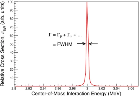
Figure 1.5: A plot of a Breit-Wigner cross section centered on 3 MeV with arbitrary values for the partial widths.
Hint is said to describe the compound-nucleus picture of the target-plus-projectile system.
The radial wavefunction for the compound nucleus,ucn(~r), can be described in terms of the single-particle wavefunctions as [Iliadis,2015]
ucni (~r) = m
X
j=1
Aijuspj (~r), (1.12)
where there are m single-particle wavefunctions and the Aij are amplitudes for the contribution of each single-particle state to the compound-nucleus state being described. Typically, a compound-nucleus wave function will be primarily described by one single-particle wave function, so all otherAij are usually ignored. Although nuclear physics theory can not predict the placement and strengths of all of the resonances in all compound-nucleus systems yet, it can be shown that if a resonance is experimentally measured at a resonance energy,Er, and is sufficiently narrow, then the cross section near the resonance energy is well-described by the Breit-Wigner cross section,
res= BW =
2
4⇡
(2J+ 1)(1 + 01)
(2j0+ 1)(2j1+ 1)
p
(Er E)2+ ( /2)2
, (1.13)
where the factor of (1 + 01) includes a Kronecker delta to create of an extra factor of 2 in the cross section
in the case of identical target and projectile nuclei. Here = 2⇡~/p2m01E is the deBroglie wavelength and
j0,j1, andJ are the spins of target, projectile, and resonance, respectively.
entrance and exit channels and total resonance width, respectively. These can be understood by analysis of Figure 1.5, which displays the Breit-Wigner cross section for a fictional resonance centered at 3 MeV with arbitrary values for and the relevant target, projectile, and resonance spins. The cross section of Figure 1.5 increases by orders of magnitude at the resonance energy with the full-width at half of the maximum (FWHM) of the cross section given by . This total width can be experimentally observed and is related to the partial widths for the available entrance and exit channels by
=X
i
i, (1.14)
with each i being the various possible entrance and exit channel partial widths. Although this connection will not be derived here, it turns out that the total resonance width for an observed narrow resonance obtained corresponding to a compound-nucleus resonance, cn, can be described in terms of the single-particle resonance widths, sp, using the same Aij coefficients that were used for the compound-nucleus wave functions above, i.e.
cn i =
n
X
j=1 A2ij
sp
j . (1.15)
The factorA2
ij is generally referred to as the spectroscopic factor and is written formally as
A2ij =C2S, (1.16)
where C is an isospin Clebsch-Gordan coefficient. Technically, S is the literal spectroscopic factor, but S
appears in multiplication withC2 often enough that the entire product is usually referred to by the same name.
1.4: Nuclear Physics in Stellar Environments
Nuclear physics processes are extremely sensitive to the energy of the interacting particles, which in turn depends on the temperature of the stellar environment, and also on the nuclear cross section, . In order to understand how nuclear physics processes occur in stars we must consider the temperature of the relevant stellar environment. Given a temperature,T, of a stellar interior, the velocity distribution of nuclei within the star is given by the Boltzmann distribution as [Iliadis,2015]
P(v)dv=⇣ m01 2⇡kT
⌘3/2
Here,m01,v, andkare the reduced mass and relative velocity of the interacting particles and the Boltzmann constant, respectively. This can be translated to the energy regime with the substitutions
E= 1
2m01v
2 & dE=m01vdv (1.18)
)P(E)dE = ⇣ m01
2⇡kT ⌘3/2
e kTE4⇡v2
✓ dE
m01v ◆
(1.19)
= ⇣ m01 2⇡kT
⌘3/2
e kTE4⇡
r 2E m01 ✓dE m01 ◆ (1.20)
P(E)dE = 2
r E
⇡
dE
(kT)3/2e
E
kT. (1.21)
The product of Avagadro’s number and the thermally averaged convolution of the nuclear cross section with the relative velocity of interacting particles is referred to as the reaction rate in nuclear astrophysics. This quantity is given by
NAh vi01 = NA
Z 1
0
v (v)P(v)dv (1.22)
= NA
Z 1
0 r
2E
m01 (E)P(E)dE (1.23)
NAh vi01 = NA
r
8 ⇡m01
1 (kT)3/2
Z 1
0
E (E)e kTEdE. (1.24)
The form of the nuclear cross section strongly depends on the mechanism by which the nuclear reaction occurs. Assuming that no interference exists between competing mechanisms, the individual contributions to the total reaction rate may be summed incoherently to calculate the total reaction rate via
NAh vitot=
X
[NAh vi]narrow
resonances +
X
[NAh vi]broad
resonances+ [NAh vi]directcapture+ [NAh vi]continuum, (1.25)
where we have contributions coming from the sum of all narrow and broad resonances, the non-resonant or direct capture (DC) rate, and the continuum. We will be concerned mainly with proton capture by means of resonant and direct proton capture processes.
1.4.1: Narrow-Resonance Reaction Rates
As discussed in Section 1.3.3, a resonance is the result of a large amplitude of the incoming particle wave function within the nuclear interior. Both broad and narrow resonances can be described by a resonant cross section, res, equivalent to the Breit-Wigner cross section shown in Equation 1.13
res=
2
4⇡
(2J+ 1)(1 + 01)
(2j0+ 1)(2j1+ 1)
p
(Er E)2+ ( /2)2
= (1 + 01) 2
4⇡!
p
(Er E)2+ ( /2)2
The parameter ! contains all factors of the form (2j+ 1). Recall that the parameters p and are the partial widths of the entrance and exit channels and = p+ +... is the total resonance width. Note that if the resonance in question is sufficiently broad, then the widths in Equation 1.26 are energy dependent quantities. However, for the narrow resonances that are considered here, the widths are assumed to be constant and to be less than a few keV.
Substitution of this Equation 1.26 into Equation 1.24 yields the resonant reaction rate equation [Iliadis, 2015]
NAh vires = NA~2
p
2⇡ (m01kT)32
!
Z 1
0
a be E/kT (Er E)2+ ( /2)2
dE (1.27)
⇡ NA~2
p
2⇡ (m01kT)32
e Er/kT!
Z 1
0
a b (Er E)2+ ( /2)2
dE, (1.28)
where we’ve used the fact that the dominant contribution to the integral occurs atE=Er. Noting that the partial and total widths are constant over a narrow resonance, we can rewrite the integral more conveniently as
NAh vires = NA~2
p
2⇡ (m01kT)32
e Er/kT!
✓
2 a b
◆ Z 1
0
/2
(Er E)2+ ( /2)2
dE (1.29)
= NA~2
p
2⇡ (m01kT)32
e Er/kT!
✓
2 a b
◆
⇡ (1.30)
= NA~2
✓
2⇡
m01kT ◆3
2
e Er/kT!
✓
a b◆
(1.31)
NAh vires = NA~2
✓
2⇡
m01kT ◆3
2
e Er/kT! . (1.32)
In the last line of the above derivation we have introduced the quantity ! , which is referred to as the resonance strength. This quantity is directly proportional to the integral of the cross section over the narrow resonance width and is generally what is reported in the literature when measurements of resonant reaction rates are made.
1.4.2: Direct-Capture Reaction Rates
Figure 1.6: Total cross section for the16O(p, )17F reaction versus center-of-mass interaction energy. This
figure is fromIliadis[2015].
advantageous to rewrite the direct-capture cross section, (E)DC, with the typical 1/Edependence and the approximate probability of s-wave transmission through the Coulomb barrier, e 2⇡⌘, explicitly written, as
shown in Equation 1.9. This leaves
(E)DC = 1
Ee
2⇡⌘S(E). (1.33)
The parameterS(E) introduced here is the astrophysical S-factor and is, essentially, the nuclear cross section with a reduced energy dependence. Recall that⌘ is the Sommerfeld parameter given by
⌘=
r m01
2E
Z0Z1e2
~2 , (1.34)
with Z0 and Z1 being the charge of the target and projectile. The quantity ⌘ contains a 1/pE energy dependence that can be easily overlooked, but is extremely important for identifying the astrophysically important energy range in a particular stellar environment. For this reason it is convenient to factor out the constant terms in⌘ and explicitly write the energy dependence as
⌘=
✓rm01
2
Z0Z1e2
~2 ◆ 1
p
E =⌘
0p1
Substituting this definition of (E)DC into Equation 1.24 yields the direct-capture reaction rate
NAh viDC=NA
r
8 ⇡m01
1 (kT)3/2
Z 1
0
S(E)exp
2⇡⌘0 p
E E
kT dE. (1.36)
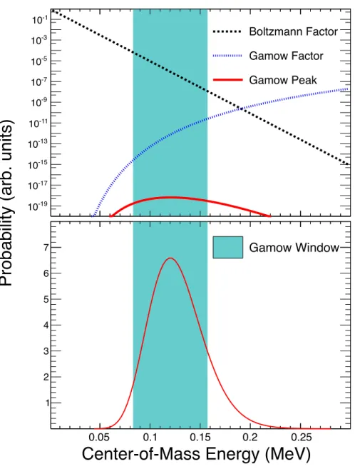
The product of exponentials in the integral severely restricts the energy range over which any significant nucleosynthesis can occur. Each of these exponential functions is plotted in Figure 1.7. To reiterate the meaning of each term, the Gamow factor,e 2⇡⌘0/pE, approximates the s-wave transmission probability for a charged particle passing through the Coulomb barrier and the Boltzmann factor, e E/kT, describes the energy distribution of particles within the stellar environment. These are shown as the black, dashed line and the blue, dotted lines on Figure 1.7, respectively. The Gamow factor drops o↵ very sharply at lower projectile energies while the Boltzmann factor decreases with increasing energy. The product of these two functions is shown in red in Figure 1.7 and is referred to as the Gamow peak. While this peak appears small on the log-scale shown in the top panel of Figure 1.7, the linear scale shown in the bottom panel of the same figure emphasizes the fact that the majority of this peak is restricted to a narrow energy region. The only non-negligible contribution to the integral comes from this energy range over which Gamow peak is non-negligible. This energy region is referred to as the Gamow window, indicated on Fig 1.7 as the shaded region, and is defined by the maximum and FWHM of a Gaussian approximation to the Gamow peak,E0
and , respectively. The calculation of this approximation will not be repeated here, but can be found in Iliadis[2015]. The result is
Gamow Window = E0± /2, (1.37)
where E0 =
⇡
~Z0Z1ekT
r m01
2
2/3
(1.38)
& = 4
r E0kT
3 . (1.39)
The majority of stellar nucleosynthesis will occur within this energy window, the position and width of which depend on the temperature of the stellar environment. The exception to this statement is the possibility of a narrow resonance, discussed earlier. If a narrow resonance exists within the Gamow window, it will likely dominate the stellar reaction rate. However, if a narrow resonance is sufficiently strong, then it may significantly contribute to the stellar reaction rate even if it exists outside of the Gamow window. 1.5: The Underlying Theme
0.05 0.1 0.15 0.2 0.25 -19
10
-17
10
-15
10
-13
10
-11
10
-9
10
-7
10
-5
10
-3
10
-1
10
Boltzmann Factor
Gamow Factor
Gamow Peak
0.05 0.1 0.15 0.2 0.25
1 2 3 4 5 6
7
Gamow Window
Probability (arb. units)
Center-of-Mass Energy (MeV)
0.05 0.1 0.15 0.2 0.25
Figure 1.7: The Gamow peak for a stellar temperature of T9 = 0.1 shown on a logarithmic scale (top) and
isotopic or elemental abundances that are unambiguously determined through nucleosynthesis calculations or more sophisticated stellar simulations, then there is an opportunity to advance the understanding and interpretation of that phenomenon. However, glaring ambiguities in the isotopic abundances resulting from stellar nucleosynthesis still arise in a large number of important nuclear burning sites. These ambiguities can sometimes be linked to, or proposed as, the source of an unexplained stellar observation or behavior. They also often imply a lack of experimental accuracy and/or precision with regard to a one or more relevant nuclear reactions. These nuclear reactions must be measured in the laboratory if the uncertain stellar site is to be understood further.
The physical measurement of a nuclear reaction requires careful preparation and analysis of the acquired data if an accurate result is to be obtained. This process is further complicated by the fact that the result of a nuclear reaction measurement is typically determined relative another stronger and more easily measured reference resonance. However, even if a perfectly measured reference resonance exists in the reaction of interest, if the characteristics of the targets used during experimentation are poorly known, then the result will su↵er from the same uncertainties. Of course, the accelerators used to provide the proton beams (used here) must also be well characterized. These issues represent some of the main pitfalls that the experimentalist is confronted with during a measurement.
The underlying theme of this entire thesis is the use of nuclear reactions to probe stellar processes. This topic is explored in two di↵erent ways and in two di↵erent stellar sites: classical novae and globular clusters. The experimental uncertainties on a large number of the nuclear reactions relevant to a particular class of novae are small enough that some very interesting connections between elemental ratios of abundances in the ejected material and the amount of mixing between outer layers of the white dwarf core and the accreted material before the explosion can be derived. These relationships are derived via calculations of the expected nucleosynthesis based on input from hydrodynamic nova models. This topic is discussed in great detail in Chapter 2 and provides new insight into the evolution of classical novae.
Globular clusters are an example of the opposite scenario regarding the quality of nuclear physics input data. Observed anti-correlations between sodium and oxygen abundances in cluster stars that can not be reproduced by stellar models point towards inaccurate or incomplete nuclear data for the relevant reactions. The22Ne(p, )23Na reaction, at stellar temperatures relevant to TP-AGB stars, is commonly believed to play
a major role in this particular abundance anomaly. Therefore, this reaction must be measured in order to better understand the evolution and nucleosynthesis of TP-AGB stars and of globular clusters. Background on this anti-correlation and on TP-AGB stellar evolution are given in Chapter 3.
majority of data acquisition in this work. Chapter 5 contains a discussion of target fabrication at the UNC Ion Implanter, Rutherford Backscattering Spectrometry experiments performed to characterize targets used in measurements of the 22Ne(p, )23Na reaction, and methods by which target degradation was monitored during the course of these experiments. Chapter 6 describes the e↵orts made to obtain a reliable reference resonance strength for measurements of the weak, low-energy resonances in22Ne(p, )23Na through a revision
of the strength of the strong, 458-keV resonance in the same reaction. Finally, Chapter 7 details the low-energy measurements of the22Ne(p, )23Na reaction that form the core of this thesis. Conclusions regarding
2: NUCLEAR MIXING METERS FOR CLASSICAL NOVAE 2.1: Preface
As mentioned in Chapter 1, a significant number of nuclear reactions important for the evolution of classical novae are known to a relatively high precision. This knowledge allows the nuclear astrophysicist to go a step further and use stellar models to learn more about the dynamics and characteristics of classical novae. This is precisely what was done inKelly et al. [2013], which is summarized and expanded upon in this chapter. This work was carried out in collaboration with Christian Iliadis, Lori N. Downen, Jordi Jos´e, and Arthur E. Champagne. Additionally, partial credit for the work described in Section 2.5 goes to Richard Longland as well. In addition to the funding sources listed in the acknowledgements section, this work was partially funded by the Spanish MICINN grants AYA2010-15685 and EUI2009-04167, the E. U. FEDER funds, and the ESF EUROCORES Program EuroGENESIS.
2.2: Introduction and Background on Classical Novae
The commonly accepted theory of classical novae involves a white dwarf of carbon-oxygen (CO) or oxygen-neon (ONe) composition accreting matter from a main sequence partner via Roche lobe overflow. The transferred matter carries angular momentum and thus forms an accretion disk. Subsequently, matter accumulates on the surface of the white dwarf under degenerate conditions [Starrfield et al., 1972, Prialnik et al.,1978]. Figures 2.1 and 2.2 show a schematic representation of the Roche lobe surrounding each star
in this binary system from [Iliadis,2015] and an artist’s rendition of a classical nova explosion, respectively. This environment leads to a thermonuclear-runaway event, similar to that described in Chapter 1, to occur during core helium ignition in which the energy released from nuclear fusion initially goes towards lifting the degeneracy of the stellar environment. However, the degeneracy lifting does not occur instantaneously, so there is a brief period of time where the temperature rises rapidly without being balanced by an increase in outward pressure. Matter is violently expelled into the interstellar medium once the degeneracy is lifted, but the underlying white dwarf star remains intact [Jos´e et al.,2006,Starrfield et al.,2008].
Figure 2.1: A schematic representation of the gravitational domains, or Roche lobes, of both stars present in a classical nova from [Iliadis, 2015]. The inner Lagrange point shown on this diagram represents the innermost point along the Roche lobe of either star where there is no net gravitational force from either star in this binary system. Roche lobe overflow occurs via mass transfer through this inner Lagrange point.
the CNO cycles. Furthermore, spectroscopic observations of large neon abundances for the most energetic classical novae, also known as neon novae, point directly to mixing between accreted matter and a white dwarf of ONe composition. Numerous physical causes of this mixing have been explored, including di↵ usion-induced mixing [Prialnik and Kovetz, 1984, Kovetz and Prialnik, 1985, Iben et al., 1991, 1992, Fujimoto and Iben,1992], shear mixing at the disk-envelope interface [Durisen,1977,Kippenhahn and Thomas,1978,
MacDonald, 1983, Livio and Truran,1987, Kutter and Sparks,1987, Sparks and Kutter,1987], convective
mixing at the core-envelope interface [Woosley, 1986,Glasner and Livne, 1995, Glasner et al., 1997, 2005, 2007,Kercek et al.,1998,1999,Casanova et al.,2010,2011a,b], and mixing by gravity wave breaking on the
white dwarf surface [Rosner et al.,2001,Alexakis et al.,2004]. However, the processes by which outer white dwarf material is mixed with the accreted envelope require further investigation.
Using one-dimensional (1D) hydrodynamic models,Downen et al.[2013] recently investigated if ratios of observed elemental abundances can be used to constrain the peak temperature during the explosion. It was found that a number of elemental ratios, including N/O, N/Al, O/S, and S/Al, show a strong monotonic dependence on the peak temperature, and thus represent useful thermometers for the explosion. Since mixing processes cannot be studied self-consistently in a 1D stellar model, a value of 50% for the degree of mixing between the white dwarf and the accreted envelope was artificially introduced prior to the explosion. This particular value is commonly used in the literature [Politano et al., 1995, Jos´e and Hernanz, 1998, Smith et al.,2002], but so far, has not been systematically constrained from spectroscopic observations.
It could be argued that the observed overall metallicity, Z, of classical novae provides exactly such a constraint. However, there are several reasons to doubt the reliability of reported metallicity values. For example, the review byGehrz et al.[1998] lists the following metallicity values obtained by di↵erent groups for the same classical nova: Z = 0.39 0.66 for V693 CrA;Z = 0.10 0.44 for QU Vul; andZ= 0.18 0.49 for V1974 Cyg. Therefore, the reported overall metallicity is not a reliable basis for estimating the degree of mixing between the outer white dwarf core and the accreted envelope. We will discuss this issue in more detail below.
A number of observations hint at useful mixing meters. First, numerous investigations have shown [see, e.g.,Jos´e and Hernanz,1998,Yaron et al.,2005,Starrfield et al.,2009,Denissenkov et al.,2013] that during explosive hydrogen burning in classical novae the peak temperatures are less than 400 MK. The reactions that can bridge the A<20 (CNO) and A 20 mass regions are very slow at these temperatures. Therefore, the total number of CNO nuclei will stay approximately constant during the explosion, and thus the CNO elemental abundance should represent a possible mixing meter [see, e.g., Kovetz and Prialnik, 1997, Jos´e and Hernanz,1998,Starrfield et al.,2009]. Second, the thermonuclear rate of the20Ne(p, )21Na reaction is
very slow at classical nova temperatures. Thus, most of the initial20Ne nuclei that are mixed from the white
dwarf into the accreted envelope survive the thermonuclear runaway. In fact, this survival of20Ne is what
first enabled the discovery of ONe novae via emission of the Ne II line [Williams et al.,1985]. Since20Ne is
expected to be the dominant neon isotope, the observed elemental neon abundance should be a promising mixing meter.
In the remainder of this chapter we carry out a systematic investigation of all elements, including CNO and neon, with abundances that can be used to constrain the degree of mixing between matter from the outer white dwarf layers and the accreted envelope in classical novae. We will focus on ONe novae because these objects display a greater variety of nuclear activity than CO novae. Also, more reliable spectroscopic abundance data exist for the former class [for the latest elemental abundance compilation, seeDownen et al., 2013]. Results obtained using a 1D hydrodynamic model are presented in Section 2.3. Following the analysis
of hydrodynamic results, the uncertainties in the nuclear physics input parameters were investigated via post-processing nucleosynthesis network calculations. These calculations are described in detail in Section 2.4. The output of these calculations can then be used to identify the reactions that must be measured in order to minimize uncertainties in the isotopic or elemental abundances from these nucleosynthesis calculations. The methods used to identify these reactions are discussed in Section 2.5. As will be seen for this particular case, it turns out that current nuclear physics uncertainties are not significant enough to induce large uncertainties in the nucleosynthesis results. Therefore, these results are sufficiently robust in their current state for comparisons to observed novae and can immediately provide insight into the behavior of classical novae. These comparisons are discussed in Section 2.6 and the impact on previous work by [Downen et al., 2013] is discussed in Section 2.7. Finally, some concluding remarks regarding chapter are given in Section
2.8.
2.3: Hydrodynamic Simulations
Table 2.1: Selected results for characteristics of hydrodynamic ONe nova models. The models were computed using the 1D hydrodynamic code SHIVA [Jos´e and Hernanz, 1998]. The mixing fraction is defined as the weight by mass of the outer white dwarf matter that has been mixed into the envelope prior to nuclear burning.
Mixing Fraction MW D(M ) Tpeak(GK) Mej(10 5M )
25%
1.15 0.218 2.12
1.25 0.238 1.70
1.30 0.256 1.18
1.35 0.306 0.429
50%
1.15 0.228 2.46
1.25 0.247 1.89
1.30 0.265 1.17
1.35 0.316 0.455
75%
1.15 0.249 2.44
1.25 0.268 1.88
1.30 0.284 1.29
1.35 0.344 0.447
of twelve hydrodynamic models of classical novae used for this work. Recall that the goal is to identify a set of mixing meters that are simultaneously insensitive to peak nova burning temperature (which is closely related to the mass of the underlying white dwarf) and strongly dependent on the mixing between the outer white dwarf layers and accreted envelope prior to thermonuclear runaway. With that goal in mind, the models encompass four di↵erent underlying white dwarf masses (1.15 M , 1.25 M , 1.30 M , and 1.35 M ) and three di↵erent mixing fractions between the outer white dwarf layers and the accreted envelope prior to the thermonuclear runaway (25%, 50%, and 75%; the mixing fraction is defined as the weight by mass of the outer white dwarf matter that has been mixed into the envelope prior to nuclear burning). The initial luminosity and mass accretion rate for all models amount to Lini = 10 2 L and ˙Macc = 2⇥10 10 M yr 1, respectively. Information on the model parameters (peak temperature, mixing fraction, and ejected
mass) is summarized in Table 2.1.
The nuclear reaction network used for hydrodynamic simulations and post-processing nucleosynthesis calculations consists of 117 nuclides ranging from1H to 48Ti, linked by 654 interactions, including all rel-evant (p, ), (p,↵), and (↵, ) reactions and weak decays. The nuclear interaction rates were adopted from recommended values provided by the STARLIB library [Sallaska et al.,2013]. For most reactions of interest to classical novae, the experimental rates contained in STARLIB have been obtained by the Monte Carlo method described in Longland et al. [2010b] and Iliadis et al. [2010b]. The library also provides the rate probability density function at temperatures in a grid ranging from 10 MK to 10 GK. This unique feature will be important for the post-processing studies, as discussed in more detail in Section 2.4.
![Figure 1.1: Hertzsprung-Russell Diagram of globular cluster M5 from Sandquist et al. [1996].](https://thumb-us.123doks.com/thumbv2/123dok_us/8317757.2204067/22.918.196.718.311.830/figure-hertzsprung-russell-diagram-globular-cluster-m-sandquist.webp)