TIME SERIES ANALYSIS OF COMPOSITIONAL DATA
USING A DYNAMIC LINEAR MODEL APPROACH
AMITABHA BHAUMIK, DIPAK K. DEY AND NALINI RAVISHANKER
Department of Statistics, University of Connecticut,
U-4120, 215 Glenbrook Road, Storrs, CT 06269, USA
Abstract. Compositional time series data com-prises of multivariate observations that at each time point are essentially proportions of a whole quantity. This kind of data occurs frequently in many disci-plines such as economics, geology and ecology. Usual multivariate statistical procedures available in the literature are not applicable for the analysis of such data since they ignore the inherent constrained na-ture of these observations as parts of a whole. This article describes new techniques for modeling com-positional time series data in a hierarchical Bayesian framework. Modified dynamic linear models are fit to compositional data via Markov chain Monte Carlo techniques. The distribution of the underlying er-rors is assumed to be a scale mixture of multivariate normals of which the multivariate normal, multivari-ate t, multivariate logistic, etc., are special cases. In particular, multivariate normal and Student-t er-ror structures are considered and compared through predictive distributions. The approach is illustrated on a data set.
Keywords. Box-Cox transformation; Composi-tional data; Hierarchical Bayesian model; Scale mix-ture of normals distribution; Student-t distribution.
1. INTRODUCTION
Compositional time series occur in many applica-tion areas including geology, manufacturing design, ecology, biology, etc. It is characterized by com-ponents which are positive and sum to one at each time point. In many cases, such compositions also change over time. In general, a G-variate composi-tional time series data consists of a G-dimensional vector of non-negative componentsWt1, ..., WtGsuch
that Wt1+...+WtG = 1 , for each t (Aitchison,
1982). Because of this unit sum constraint at each time t, the composition can be completely defined by any of the g = G−1 components so that the vector Wt = (Wt1, ..., WtG)0 lies in a g-dimensional
simplex which is defined as
Sgt ={(Wt1, ..., Wtg) :Wt1≥0, ..., Wtg ≥0; Wt1+...+Wtg = 1}. (1)
Statistical analysis of such constrained multivariate time series in the presence of covariate information is very useful in practice. However, the biggest hin-drance to the analysis of compositional data arises from the two inherent constraints mentioned above. Standard techniques such as regression with vec-tor auvec-toregressive moving average (VARMA) errors, or Kalman filtering (Kalman, 1969), etc., are not directly applicable to raw compositional time se-ries data. To circumvent this problem, Aitchison’s (1982) proposal was to transform data from theg -dimensional simplex to theg-dimensional real space
Rg, and to employ an additive error model. The
most popular transformation is the Additive Log Ratio (ALR) transformation, which is of the form
Yti = log(Wti/WtG), i = 1, ..., g. Another
possibil-ity is the Box-Cox transformation (Box and Cox, 1964) which was used for cross-sectional composi-tional data by Rayens and Srinivasan (1991a, b) in a frequentist setup and by Iyenger and Dey (1998) in a Bayesian framework. In both cases, the trans-formed variable may be assumed to follow a multi-variate normal distribution. The Box-Cox transfor-mation is more general in the sense that the ALR transformation is a special case.
Literature is sparse on compositional analysis of multivariate time series incorporating covariate in-formation. Quintana and West (1988) used an ALR transformation with multivariate dynamic lin-ear models. A state space model based on the Dirichlet distribution was developed by Grunwald, Raftery and Guttorp (1993). In this article, we an-alyze compositional time series data after a Box-Cox transformation. Inference is carried out in the Bayesian framework using a very rich class of scale mixture of multivariate normals (SMMVN) for mod-eling the errors. This class of distributions includes the multivariate normal, Student-t, logistic, stable etc. (see Dey and Chen, 1998). In this article, we in-vestigate the performance of the multivariate normal
and multivariate Student-t distributions in particu-lar. Model performance is assessed via predictive distributions; the Conditional Predictive Ordinate (CPO) is computed and is used for model assess-ment.
The format of the paper is as follows. In section 2 we discuss the proposed model. Predictive distribu-tions and their Monte Carlo estimates are also dis-cussed. Section 3 presents an illustration. It consists of compositions of vehicles produced by USA, Japan and other countries over the time period 1947-1987. Section 4 contains some concluding remarks.
2. A MODEL FOR TRANSFORMED COMPOSITIONS
Let Wt denote the G-dimensional composition at
time t as defined in section 1. We assume that
Wt depends on some unknown state of natureηt=
(ηt1, ..., ηtG), a vector of true proportions. Due
to the unit sum constraint, Wt’s are points on a g=G−1 dimensional simplex. The Box-Cox trans-formation ofWttransforms the vector toYtin Rg:
Yti= (WtGWti)λti−1 λti ifλti6= 0 log(Wti WtG) ifλti= 0 , (2) where λti ∈ R is an unknown parameter known as
the Box-Cox parameter, t = 1, ...., T , i = 1, ...., g
and g =G−1. This transformation is denoted in this paper asYt=BC(Wt, λt), as a special case of
which we get ALR transformation when λti= 0 for
alli, t.
2.1. The Dynamic Linear Model
Let Xt denote the l?-dimensional covariate vector
at time t. The linear regression model for the g -dimensional time seriesYthas the form
Yt|λt=αt+Xtβt+et (3)
where the unknown parameters αt and βt are g
-dimensional vectors, λt denotes the vector of
Box-Cox parameters, and et is the random error. This
model is investigated under the scale mixture of mul-tivariate normals (SMMVN) error distribution. Sup-pose et is normally distributed with mean 0 and
unknown variance k(τ)Vt, where k(τ) is a positive
function of the mixing parameter τ, where τ has pdf g(τ). When k(τ) = τ, and τ has a degener-ate distribution at 1, it is well known that et has
a multivariate normal distribution with mean 0 and
varianceVt. Whenk(τ) = 1/τ,and the mixing
den-sityg(τ) is Gamma with both location and scale pa-rameter equal toν/2, the marginal distribution ofet
becomes Student-t, with location parameter 0, scale parameterτ Vtand degrees of freedom ν. While the
multivariate normal error model is simple to fit, the multivariate Student-t distribution handles extreme observations better. The observation equation can be rewritten as
Yt|λt=Ztηt+et, (4)
whereZt= (1 Xt) is ag×l vector of covariates at
time tandηt= (αt,βt)0 is anl-dimensional vector,
forl=l?+ 1.
The essential difference between the dynamic lin-ear model and the static linlin-ear model is that in the former case, the regression coefficients are not as-sumed to be constant, but may change with time. This dynamic feature is incorporated via the system equation
ηt=Gηt−1+wt, (5)
where G is a known matrix, and we assume that
p(wt|Wt) is normal, i.e.,
wt∼N(0, Wt). (6)
It is assumed that the unknown, time-dependent Box-Cox parameter follows the system equation
λt=Hλt−1+ut, (7)
where p(ut|Ut) is normal, i.e.,
ut∼N(0, Ut). (8)
Under this modeling framework, the system equa-tion and the equaequa-tion on the Box-Cox parameter can be reparametrized as ηt = t X i=1 Gt−iwi (9) λt = t X i=1 Ht−iu i, (10)
whereGt−i andHt−iare thet−ithpowers ofGand H respectively. Rewriting the observation equation using these transformed parametric expressions, the model has the form
Yt|λt = Zt t X i=1 Gt−iw i+et (11) λt = t X i=1 Ht−iu i, (12) where Yt|λt = BC(Wt, λt). In addition to
the usual linear model assumptions regarding the error terms, we also postulate that et
and ut are independent of wt. Let µt = Zt Pt i=1Gt−iwi,Y=(Y1, ..., YT) 0 ,V=(V1, ..., VT) 0 , W=(W1, ..., WT) 0 andU=(U1, ..., UT) 0 .
2.2. Posterior Distribution and Model Fit
The exact likelihood has the form
L(Y;V, W, U, τ)∝exp[− 1 2k(τ) T X t=1 (BC(Wt, u1, ... .., ut)−µt) 0 V−1 t ×(BC(Wt, u1, ..., ut)−µt)]×g(τ) ×exp[−1 2ut 0 Ut−1ut]×exp[−1 2wt 0 Wt−1wt] × T Y t=1 |Vt|− 1 2|Ut|−12|Wt|−12.
In the special case when the mixing parameter has a Gamma distribution with both the location and scale parameters ν/2 for known ν, the likelihood function becomes, L(Y;V, W, U)∝[1 + (BC(Wt, u1, u2, ..., ut)−µt) 0 V−1 t ×(BC(Wt, u1, u2, ..., ut)−µt)/v]−[(v+g)/2] ×exp[−1 2ut 0 Ut−1ut] exp[−1 2wt 0 Wt−1wt] × T Y t=1 |Vt|− 1 2|Ut|−12|Wt|−12.
For the prior specification, we assume that p(w1)
and p(u1) are N(aw, Rw) and N(au, Ru)
distribu-tions respectively with pre-specified hyperparame-tersaw, au, Rw and Ru. The prior specifications on
the covariance matrices are assumed to be of the form
π(Vt, Wt, Ut) =π(Vt)π(Wt)π(Ut), (13)
where π(Vt), π(Wt) and π(Ut) are inverse Wishart
distributions with known hyperparameters. A rou-tine sensitivity analysis may be carried out in order
to investigate the effect of these hyperparameters on the model fit. By Bayes’ theorem, the joint posterior density is then π(u, V, W, U, τ|Y)∝L(Y;V, W, U, τ) × T Y t=1 π(Vt, Wt, Ut)× T Y t=2 p(wt|Wt)p(ut|Ut) ×p(w1)p(u1)g(τ).
The resulting joint posterior is analytically in-tractable. The full conditional distributions of the parameters are proportional to the joint posterior and do not have standard forms. We have em-ployed a sampling based approach via Gibbs sam-pling (Gelfand and Smith, 1990), with the Metropo-lis Hastings algorithm (Hastings, 1970) using a Gaussian proposal. Maximum likelihood estimates of the parameters provide the initial values for the sampler. Let (η(s), λ(s)),s= 1, ..., B denote
conver-gent samples generated from the joint posterior. The means and standard deviations of these samples cor-responding to each parameter provide summary fea-tures of the marginal posterior distributions. Sam-ples of estimated expected composition proportions can also be calculated at each time point for given covariates. Fors= 1, ..., B, these are
b η(tis)= h λ(tis)Ybti(s)+ 1 i1/λ(tis) 1 +Pgi=1hλti(s)Ybti(s)+ 1i1/λ (s) ti , i= 1, ..., g (14) and fori=G b η(tGs)= 1 1 +Pgi=1 h λ(tis)Ybti(s)+ 1 i1/λ(tis) (15)
where λ(tis) and Ybti(s) are calculated from the given model. Estimates of these expected proportions are obtained as the Monte Carlo averages of the expres-sions in (14) and (15) over theB samples.
Convex credible regions for proportions can also be constructed. The first step is to generate a sam-ple of B proportions at each time pointt= 1, ..., T. At time pointt, thesthsample for theithproportion
is given by equation (14) and (15). These 100(1−α) credible regions indicate how the shapes of the sim-plexes corresponding to the true proportions change over time. These regions are obtained using the SPlus function chull, which returns the indices of
the points belonging to the hull. The peel option permits peeling off from the convex hull successively until either all the planar points are assigned or until a user-specified limit is reached.
2.3. Cross Validation
In this article, model assessment is based on the cross-validation predictive density. It is well known that the marginal density of f(Y) is equivalent to the set {f(Yr|Y(r)) : r = 1,2, ...., T}, where
f(Yr|Y(r)) is the predictive distribution ofYr when
the rth observation is deleted. The expression for f(Yr|Y(r)) is f(Yr|Y(r)) = f(Y) f(Y(r)) = Z f(Yr|η, Y(r),Z) π(η|Y(r))dη, (16)
which is called the Conditional Predictive Ordinate (CPO). Using the samplesη(s), s= 1,2, ...., B
gen-erated from the posterior, the Monte Carlo estimate of CPO can be calculated as (Dey, Chang and Ray, 1996) CPOr=B ÃB X s=1 1 f(yr|η(s), Y(r)) !−1 . (17)
For the purpose of model checking, the presence of many small CPO’s criticizes the model. A useful summary statistic of the CPO’s is the logarithm of the pseudo-Bayes factor (Geisser and Eddy, 1979 and Dey, Chen and Chang, 1997), defined as
P sBF =
T X r=1
log(CPOr). (18)
The advantage of P sBF over the Bayes factor (Gelfand and Dey, 1992) as a model assessment tool is that the latter is not well defined with improper priors, and is generally quite sensitive to vague proper priors. The evaluation of f(yr|η(s), Y(r)) is
complicated in time series models. The calculation is simplified as follows (Pai and Ravishanker, 1996):
f(yr|η(s), Y(r))∝
T Y i=t
fi(yi|yi−1, ..., y1, η), (19)
and facilitates model assessment.
3. ILLUSTRATION
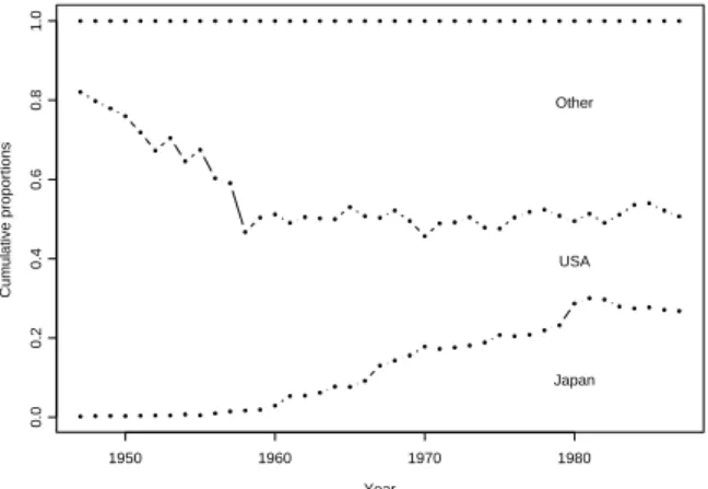
We analyze trivariate compositional data of motor vehicle production, consisting of the number of mo-tor vehicles produced by USA, Japan and Other countries between 1947 and 1987 (see Grunwald, Raftery and Guttorp, 1993). Data on the move-ment of the US economy, measured by the percent-age change in US Gross National Product (GNP) is a covariate. Year Cumulative proportions 1950 1960 1970 1980 0.0 0.2 0.4 0.6 0.8 1.0 Japan USA Other
Figure 1. Proportion of motor vehicle production from three sources over time.
Figure 1 shows the changes in the proportions of to-tal motor vehicle production in the three categories over time. Of the three sources, the change in the Japanese production is most significant. Japan ac-counted for around one third of the total production in 1987 while their contribution in 1947 was only around 0.002% of the total. The range of the US production is (4796, 12900), indicating a production growth over time, but with a sharp decrease in con-tribution to total production. Overall, the motor vehicle production appears to be correlated with US growth rate, and there is evidence of some nonlinear relationship. Visual examination of the scatter plots of production from the three sources versus move-ment of the US economy suggests that whereas US production is positively correlated with the covari-ate, the relationship between the production from Japan and from Other countries and the covariate is only slightly positive, with a trace of nonlinear relationship. Observed behavioral differences in the three sources indicate the usefulness of a composi-tional time series analysis. Details from fitting the dynamic regression model which describes the ef-fect of US growth rate on the Box-Cox transformed motor vehicle production data from three different
sources is presented here. Model 1 corresponds to the dynamic regression model with normal errors, while Model 2 corresponds to the dynamic regression model with Student-terrors. Details of the posterior estimates fort= 41 are given in Table I.
Table I
Posterior Means and Standard Deviations of Parameters under Normal and
Student-t errors Parameter Model 1 Mean Stdev Model 2 Mean Stdev λJapan -0.4917 0.1699 -0.4889 0.1777 λUSA -0.3393 0.1717 -0.3425 0.1748 αJapan -0.0059 0.0009 0.0062 0.0009 αUSA -0.0025 0.0009 0.0003 0.0009 βJapan -0.5352 0.2007 -0.5356 0.2207 βUSA -0.3593 0.2031 -0.3503 0.2151 It is clear that the Box-Cox transformed vehicle pro-duction has significant negative relationship with US economic growth rate. Values of P sBF are -528.656 for the normal error model and -576.29 for the Student-t error model, indicating that the nor-mal error assumption provides a better fit. This is substantiated by a plot of the logarithm of CPO ra-tios; all points in the plot of log(CPO from Model 1/CPO from Model 2) are above 0.
-0.05 0.00 0.05 0.10 Japan 0.60 0.65 0.70 0.75 USA Time = 10 0.14 0.16 0.18 0.20 0.22 0.24 0.26 0.28 Japan 0.22 0.24 0.26 0.28 0.30 0.32 USA Time = 30 -0.05 0.00 0.05 0.10 Japan 0.26 0.28 0.30 0.32 0.34 0.36 0.38 Other countries Time = 10 0.14 0.16 0.18 0.20 0.22 0.24 0.26 0.28 Japan 0.48 0.50 0.52 0.54 0.56 Other countries Time = 30 0.60 0.65 0.70 0.75 USA 0.26 0.28 0.30 0.32 0.34 0.36 0.38 Other countries Time = 10 0.22 0.24 0.26 0.28 0.30 0.32 USA 0.48 0.50 0.52 0.54 0.56 Other countries Time = 30
Figure 2. Credible regions for true proportions from Model 1
0.10 0.12 0.14 0.16 0.18 0.20 0.22 0.24
Coefficients of Intercept for Japan
0.0
0.1
0.2
Coefficients of US GNP for Japan
Time = 10
-0.02 0.00 0.02 0.04 0.06 0.08 0.10
Coefficients of Intercept for Japan
-0.7 -0.6 -0.5 -0.4 -0.3 -0.2 -0.1
Coefficients of US GNP for Japan
Time = 20
-0.04 -0.02 0.00 0.02 0.04 0.06 0.08
Coefficients of Intercept for Japan
-0.8 -0.7 -0.6 -0.5 -0.4 -0.3 -0.2
Coefficients of US GNP for Japan
Time = 30
-0.08 -0.06 -0.04 -0.02 -0.00 0.02 0.04 0.06
Coefficients of Intercept for USA
-0.6
-0.5
-0.4
-0.3
Coefficients of US GNP for USA
Time = 10
-0.04 -0.02 0.00 0.02 0.04
Coefficients of Intercept for USA
-0.7
-0.6
-0.5
-0.4
-0.3
Coefficients of US GNP for USA
Time = 20
-0.10 -0.05 0.00 0.05
Coefficients of Intercept for USA
-0.8
-0.6
-0.4
-0.2
0.0
Coefficients of US GNP for USA
Time = 30
Figure 3. Convex hull for the intercept and US GNP coefficient under Model 1
The estimated convex credible regions at two se-lected time points for the true proportions corre-sponding to Model 1 are shown in Figure 2. It indicates that the relationship between the propor-tion of vehicle producpropor-tion in USA, Japan and the Other countries do not change considerably. Figure 3 shows the 95% joint credible sets for the intercept and US GNP under Model 1 at three selected time points. Column 1 corresponds to Japan and col-umn 2 corresponds to USA. The figure indicates the presence of a slow change in the shape of the credi-ble sets over time. We observed that this change is less severe for Model 2, corresponding to Student-t
errors.
4. CONCLUDING REMARKS
A regression model with a dynamic structure for pa-rameter evolution over time is used to analyze com-positional time series data. The inherent constraint in compositional data is overcome by the Box-Cox transformation which is a more general version of the ALR transformation. In our modeling framework, we incorporate flexibility in two ways. The first is via a more general class of transformations from the simplex, and the second is through the dynamic lin-ear model framework. Our model thereby incorpo-rates a possible change in the underlying mechanism. The Bayesian methodology facilitates parametric in-ference of the resulting complex model.
REFERENCES
Aitchison, J. (1982) The Statistical Analysis of Computational Data with discussion. J. R.
Statist. Soc. B, 44, 139-177.
Aitchison, J. (1986) The Statistical Analysis of
Compositional Data. London: Chapman and
Hall.
Box, G. E. P.andCox, D. R.(1964) An Analysis of Transformations. J. R. Statist. Soc. B, 26, 211-252.
Chen, M. H. and Dey, D. K. (1998) Bayesian modeling of correlated binary responses via scale mixture of multivariate normal link func-tions. Sankhya, 60, 322-343.
Dey, D. K.andBirmiwal, L. R.(1991) On Iden-tifying Mixing Density of Scale Mixtures of Nor-mal Distributions. Technical Report, Depart-ment of Statistics, University of Connecticut.
Dey, D. K.;Chang, H.andRay, S. C.(1996) A Bayesian Approach in Model Selection for the Binary Response Data. Advances in Economet-rics, 11, 145-175.
Dey, D. K.;Chen, M. H.andChang, H.(1997) Bayesian approach for the nonlinear random ef-fects models. Biometrics, 53, 1293-1252.
Gelfand, a, e. andDey, D. K.(1994) Bayesian model choice: asymptotics and exact calcula-tions. J. R. Statist. Soc. B, 56, 501-514.
Geisser, S.(1993)Predictive Inference: An
Intro-duction, Chapman and Hall: London.
Geisser, S. and Eddy, W. (1979) A predictive approach to model selection. J. Amer. Statist.
Assoc., 74, 153-160.
Gelfand, A. E.; Dey, D. K. and Chang, H. (1992) Model Determination using Pre-dictive Distribution with Implementation via Sampling-Based Methods. Bayesian Statistics
: J. M. Bernardo, J. O. Berger, A. P. Dawid and A. F. M. Smith (Eds.), Oxford University Press, 147-167.
Gelfand, A. E. and Smith, A. F. M. (1990) Sampling based approaches to calculating marginal densities. J. Amer. Statist. Assoc., 85, 398-409.
Grunwald, G. K.; Raftery, A. E. and Gut-torp, P. (1993) Time Series of Continuous Proportions. J. R. Statist. Soc. B, 55, 103-116.
Hastings, W. K. (1970) Monte Carlo sampling methods using Markov chains and their appli-cations. Biometrika, 57, 97-109.
Iyenger, M. and Dey, D. K. (1998) Box-Cox transformation in Bayesian analysis of compo-sitional data. Environmetrics, 9, 657-671.
Kalman, R. E.(1969) A New Approach to Linear Filtering and Predicting Problems. J. of Basic
Engineering, 82, 34-45.
Pai, J. S.andRavishanker, N.(1996) Bayesian Modelling of ARFIMA Processes by Markov Chain Monte Carlo Methods. J. of Forecasting, 15, 63-82.
Quintana, J. M.andWest, M.(1988) Time Se-ries Analysis of Compositional Data. Bayesian
Statistics : J. M. Bernardo, M. H. DeGroot, D.
V. Lindley and A. F. M. Smith (Eds.), Oxford University Press.
Rayens, W. S.andSrinivasan, C.(1991 a) Box-Cox Transformations in the Analysis of Compo-sitional Data. J. of Chemometrics, 5, 227-239.
Rayens, W. S.andSrinivasan, C.(1991 b) Es-timation in Compositional Data Analysis. J. of
Chemometrics, 5, 361-374.
West, M.andHarrison, P. J.(1997)Bayesian
Forecasting and Dynamic Models, Second