ON THE ESTIMATION OF DISTANCE DISTRIBUTION FUNCTIONS FOR POINT PROCESSES AND RANDOM SETS

ON THE ESTIMATION OF DISTANCE DISTRIBUTION FUNCTIONS

FOR POINT PROCESSES AND RANDOM SETS

D

S

H

S

A

´

T

T

M

1_{Institut f¨ur Stochastik, TU Bergakademie Freiberg, 09596 Freiberg, Germany;}2_{Institut f¨ur Pathologie,}

Universit¨at Ulm, Germany

E-mail: [email protected] (Accepted March 6, 2001)

ABSTRACT

This paper discusses various estimators for the nearest neighbour distance distribution function D of a stationary point process and for the quadratic contact distribution function Hqof a stationary random closed set. It recommends the use of Hanisch’s estimator of D, which is of Horvitz-Thompson type, and the minus-sampling estimator of Hq. This recommendation is based on simulations for Poisson processes and Boolean models.

Keywords: contact distribution, Horvitz-Thompson, estimator, minus-sampling, nearest neighbour distance distribution

INTRODUCTION

Random sets are successful models for various spatial structures such as porous media, phases in two- or multi-phase materials or biological tissues. They are studied in many stereological studies. In their statistical analysis, contact distributions play an important role, see Serra (1982), Stoyan, Kendall and Mecke (1995), and Ohser and M¨ucklich (2000). Of particular interest are the linear, spherical and quadratic contact distribution function (cdf) H_l;Hs

and Hq. For a stationary random closed set X , the

spherical cdf Hs is the distribution function of the

random distance from an arbitrary point outside of X to its nearest neighbour in X . The quadratic cdf Hq

is the distribution function of an analogous distance but measured in a Minkowski metric where the unit sphere is the unit cube. It is of particular value in the statistical analysis of pixel images, where the square-based metric is natural. The cdf’s characterize in some sense the size of the complement Xc _{of X , as}

introduced by Delfiner (1972). If, in the case of a porous medium, X is a model for the matrix, then Xc

is the union of all pores and the cdf’s characterize the size of the pores.

The spherical cdf is also used in point process statistics, see Diggle (1983), where often the character F is used. Perhaps still more important for point processes is the nearest neighbour distance distribution function D (or G is Diggle’s notation), which does not have a counterpart for general random closed sets.

The cdf’s and D play an important role in the characterization of the variablity of spatial

structures. They are sometimes considered in second-order stereology though they are not second-second-order characteristics in the classical use of the term ‘second-order’ in probability and statistics.

For the statistical estimation of D and of cdf’s there exist various methods, see Stoyan, Kendall and Mecke (1995). The classical estimators are minus-sampling or border estimators. Following Hanisch (1984) and Chiu and Stoyan (1998), the approach of Horvitz-Thompson (see Overton and Strehman, 1995) can be used, what leads to refined estimators. Finally Kaplan-Meier-like estimation is possible, see Baddeley and Gill (1997).

All these estimators are ratio estimators, which contain in the denominator an unbiased estimator of area fraction p or intensity λ. In the classical estimation procedure, p andλ is estimated from the whole window of observation, while the numerator is obtained only from a subwindow or by some form of edge correction. Consequently, numerator and denominator may show little correlation and are estimated with different precision. Thus it seems to be natural to ask for estimators where numerator and denumerator are (more) positively correlated and their precision is closer, even if this leads to a loss of precision of the denominator. A possible approach is to use adapted estimators of p andλ. Such a modification of classical ratio estimators has been shown to be very successful in the estimation of second-order characteristics such as the pair correlation function of random sets (Mattfeldt and Stoyan, 2000) and of point processes (Landy and Szalay, 1993, and Stoyan and Stoyan, 2000).

estimation of D and cdf’s. The present paper discusses such estimators for D and Hq and compares their

behaviour with that of the classical minus-sampling estimators. Since it is obviously very complicated to do rigorous calculations, which are very difficult even in the particular case of a Poisson process, the behaviour of these estimators is investigated by Monte Carlo simulations.

Simulations for Poisson processes, a cluster process and Boolean models lead to a clear result: For D the Horvitz-Thompson estimator introduced by Hanisch (1984) should be used, while for Hq all the

more sophisticated estimators are not better than the classical minus-sampling estimator if the criterion is the mean squared error.

ESTIMATORS OF THE NEAREST

NEIGHBOUR DISTANCE

DISTRIBUTION FUNCTION D

VARIOUS D ESTIMATORS

The function D is the distribution function of the distance from a typical point of the analysed point processΦinR

d _{to its nearest neighbour, see Stoyan,}

Kendall and Mecke (1995). Φ is assumed to be stationary and to have intensity λ. It is observed in a sampling window W , which is a compact convex set of positive volume ν_d(W). In the case of a Poisson

process of intensityλ;D(r)has the form

D(r)=1 exp( λb

dr d

) for r0;

where b_ddenotes the volume of the unit sphere ofR

d_.

Before starting with the explanation of estimators of D, it is helpful to give all points ofΦin W two real-valued marks s and c. For a fixed point x;s(x)denotes

the distance from x to its nearest neighbour in W and c(x)is the distance from x to the edge of W .

The classical and perhaps most natural estimator of D is the minus-sampling or border-method estimator

ˆ Dm,

ˆ

Dm(r)=

∑

[x;s]

1_{W b}

(o;r) (x)1

(o;r]

(s)=Φ(W b(o;r)) (1)

for r0;

where the sum in the numerator yields the number of points in the reduced window W b(o;r)with nearest

neighbour closer than r and the denominator is the total number of points in W b(o;r).

The summation goes here and elsewhere in this section over all marked point pairs [x; s] of Φ. The

structure of this estimator may be clarified by writing the denominator as

∑

[x;s]

1_{W b}

(o;r) (x):

The estimator ˆDm is frequently used and yields for

samples not too small acceptable or good results, see also below. As a function of r;Dˆm(r)is not necessarily

monotonous, see Fig. 4.14 in Stoyan, Kendall & Mecke (1995) and Fig. 9 in Baddeley et al. (1993).

Formula (1) can be rewritten as

ˆ Dm(r)=

Dm(r)

ˆ

λm(r)

(2)

with

Dm(r)=

∑

[x;s]

1_{W b}

(o;r) (x)1

(0;r] (s)

νd(W b(o;r))

and

ˆ

λm(r)=

Φ(W b(o;r))

νd(W b(o;r)) ;

whereν_d(W b(o;r))is the volume of W b(o;r).

Obviously, ˆλm(r) is an unbiased estimator of λ,

which could be called the minus-weighted estimator of intensityλ, and Dm(r) is an unbiased estimator of

λD(r). Thus, ˆDm(r) is a ratio-unbiased estimator of

D(r) of the type described in the introduction, with

adapted intensity estimator. One can expect positive correlation, between Dm(r)and ˆλm(r), i.e., large values

of Dm(r) are connected with large values of λm(r).

This relationship reduces fluctuations of ˆDm(r) and

explains the good experience with the border-method estimator. Note that it does not help if the true value ofλ would be known; replacing ˆλm(r) byλ leads to

much larger squared deviations in the estimation of D(r).

The Hanisch estimator of D(r)uses all points in W

with nearest neighbour in W and is defined as

ˆ D_H(r)=

D_H(r)

ˆ

λH

(3)

with

D_H(r)=

∑

[x;s]

1_{W b}

(o;s) (x)1

(0;r] (s)

νd(W b(o;s))

or

D_H(r)=

∑

1

[0;c) (s)1

(0;r] (s)

and

ˆ

λH=

∑

1_{W b}

(o;s) (x)

νd(W b(o;s)) :

(

ˆ

λH is pracically the same as D4(R) on page 140

of Stoyan, Kendall & Mecke, 1995). D_H(r) is an

unbiased estimator of λD(r), and ˆλ

H is an adapted

unbiased estimator of λ. D_H(r) counts all points x

with s(x) <c(x) weighted by the volume ν

d(W

b(o;s(x))); it is so organized that it can be really

determined using the information in the sampling window W . While ˆD_H(r)appeared in Hanisch (1984)

as an ad hoc estimator, Baddeley (1998) showed that it is a Horvitz-Thompson estimator.

The intensity estimator ˆλH is independent of r.

This guarantees that ˆD_H(r) is monotonous in r. The

authors do not know whether there is an estimator ofλ which is better adapted to DH(r)and produces better

estimates of D(r).

Unfortunately, Hanisch (1984) had presented (perhaps following a wrong recommendation by the first author D.S.) together with ˆD_H(r)(his formula (4))

also other D-estimators, for example

ˆ DN(r)=

∑

[x;s]

1_{W b}

(o;s) (x)1

[0;r] (s)

∑

[x;s]

1_{W b}

(o;s) (x)

:

Just this estimator appeared later in Cressie (1991), p. 638, and was also used in Baddeley et al. (1993). It is not an unbiased estimator and also not a ratio-unbiased estimator. As simulations showed (see below), it has a large squared deviation and it should be forgotten.

COMPARISON OF D ESTIMATORS

In order to compare and to evaluate the various estimators(Dˆm;Dˆ

Nand ˆDH), they were applied to each

1000 simulated point patterns in the unit square and cube ofR

2 _and

R

3_{, respectively.}

For Poisson processes of intensities λ = 50, 100 and 200 the following results were obtained. The biases of ˆDmand ˆDH in the planar and spatial cases are

small, typically negative, usually in the order of 0.001 . . . 0.005. They are smaller for d = 2 than for d = 3 and smaller for ˆD_H than for ˆDm.

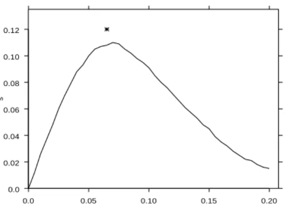
Fig. 1 shows the estimation standard deviation s(r)

for the Hanisch estimator ˆD_Hin dependence on r forλ = 50. The behaviour forλ = 100 andλ = 200 and for the spatial case is similar, the values decrease (for fixed

window) with growing intensity λ or point number probably in proportionality to 1=

p

λ. The estimation standard deviations for ˆDm are similar. The form of

the s(r)-curve shown in Fig. 1 is quite natural: For

r=0, where D(r)and all its estimators vanish, and for

large r, where D(r)and its estimators are close to one,

there is no much room for fluctuations, which appear for medium values of r.

For ˆD_N quite large biases appear. The maximum values are 0.068 (λ = 50), 0.044 (λ = 100) and 0.027 (λ= 200) in the planar case (d = 2) and 0.159 (λ= 50), 0.124 (λ = 100) and 0.100 (λ = 200) in the spatial case (d = 3).

As an example of a non-Poisson point process, a planar Gauss-Poisson process (as in Stoyan, Kendall & Mecke, 1995, p. 161) with parameters λp =

λ;p

1 = p

2= p

3 =1=3 and inter-pair distance 0.15

was analysed. This process belongs to the few number of processes which are not Poisson processes but for which there are known formulas for D(r). It is a

Neyman-Scott cluster process with empty clusters, ‘clusters’ consisting of a single point and two-point clusters with constant distance between the points.

For this process, the biases turned out to be a bit larger than for the Poisson process, but the standard deviations s(r) for the Hanisch estimator are quite

similar to those for the planar Poisson process of equal intensity. The star in Fig. 1 marks the maximum of s(r)

for ˆDH(r) in the Gauss-Poisson process case andλ =

50. Also here the biases for ˆD_N are much larger than for ˆDm and ˆDH.

r

s

0.0 0.05 0.10 0.15 0.20

0.0 0.02 0.04 0.06 0.08 0.10 0.12

Fig. 1: Estimation standard deviation s(r) for the

Hanisch estimator ˆD_Hin the case of a Poisson process in dependence on r forλ = 50. Star: maximum of s(r)

for Gauss-Poisson.

Concluding, we recommend the use of the Hanisch estimator DˆH(r) in the form (3). It

Stoyan & Stoyan (1994), p. 296 (replace β there by

βi).

ESTIMATORS OF CONTACT

DISTRIBUTION FUNCTIONS

VARIOUS CONTACT DISTRIBUTION ESTIMATORS

Contact distribution functions (cdf’s) are frequently used in the statistical analysis of point processes as well as random closed sets. In this section we concentrate on the case of random closed sets with positive volume fraction. As a practically important particular case the quadratic cdf Hq is considered,

which is of special interest in statistical analyses of pixel images.

Let X be a stationary random closed set in R

d_.

Its volume fraction p satisfies p=P(o2X), where

o denotes the origin. It is assumed that p>0. The

quadratic cdf is defined as

Hq(r) = 1 P(o62Xq˘(r)jo62X)

= 1 P(o62Xq˘(r))=(1 p)

where q(r) is the cube of side length r with one

vertex in o and sides emanating in o along the positive coordinate axes; it is ˘q(r)= q(r).

For the case of a Boolean model the formulas in Stoyan, Kendall and Mecke (1995), p 79-81, lead to explicit expressions for Hq(r). In particular, if in the

planar case the primary grains are isotropic squares of side length a (for this case the simulations were carried out), then

Hq(r)=1 exp

λ

8a

π r+r

2

for r0 (4)

whereλ denotes the intensity of the germ process.

The classical minus-sampling or border-method estimator of Hq(r)is

ˆ

Hq(r)=1 ∆(r) (5)

with

∆(r)=

νd((W q(r))\(Xq˘(r))

c

)

νd(W q(r))

νd(W\X

c

)

νd(W)

: (6)

Note that formula (6.3.6) in Stoyan, Kendall and Mecke (1995) is corrected here. The term ν_d(W\

Xc)=ν

d(W)is the usual estimator of 1 p.

The estimator ˆHq(r)will be compared with another

estimator of Hq(r), namely ˆH

a

q(r). It differs from ˆHq(r)

by different handling with volume fraction p: ˆHqa(r)

uses an adapted estimator of p, namely

ˆ p(r)=ν

d(W q(r)\X)=ν

d(W q(r));

which is of the same nature as ˆλm(r) above and

intensity estimators used in the context of second-order characteristics.

Consequently, it is

ˆ

H_qa(r)=1 ∆

a

(r) (7)

with

∆a

(r)=

νd((W q(r))\(Xq˘(r))

c

)

νd(W q(r)\X

c

)

: (8)

Furthermore, two estimators are considered which follow the Horvitz-Thompson idea, see Stoyan, Kendall and Mecke (1995), p. 215, and Chiu and Stoyan (1998),

ˆ

HqHT(r)= Z

W

1_{W q}

(d(x)) (x)1

(0;r] (d(x))

νd(W q(d(x)))

dx=(1 ˆp

HT

)

where

1 pˆHT = Z

W

1_{W q}

(d(x)) (x)1

Xc(x)

νd(W q(d(x)))

dx

and ˆHHT;a

q (r) is defined as ˆH

HT

q (r)but with the term

ˆ

p(r)from above. Here, d(x)denotes the distance from

x to X measured in the metric corresponding to the unit cube. For a given pixel image, the integrals are replaced by sums in a natural way.

Four of the estimators introduced above were compared for a long series of simulated stationary and isotropic planar Boolean models. For each case the primary grains were isotropic congruent rectangles; the same rectangular primary grain was combined with a series of germ process intensities λ; see Mattfeldt and Stoyan (2000) for more details. In total, 200 series with each 100 replications were simulated in a 512

COMPARISON OF THE CONTACT DISTRIBUTION FUNCTIONS ESTIMATORS

The results for all simulations were similar: There are no significant differences between the four estimators, the simple minus-sampling estimator is even a little better than the competitors if the mse (mean squared deviation of estimator from true value) is used as quality measure.

We give here details for the particular case of square primary grains of side length 20. In Table 1, the square roots of the mse’s of ˆHq(r)are given for various

values ofλ and in comparison to the best competitor under the other estimators.

The values of r were chosen as integers and such that Hq(r) takes small, medium and large (close to 1)

values. As a function of r the mse behaves similarly as s(r)in Fig. 1, in particular it has small values for small

and large r.

Obviously, the simple minus-sampling estimator is preferable because of its quality and conceptional simplicity.

Table 1: Square roots of mean squared deviations of estimators from true values (mse)

λ r Hˆq(r) competitor

0.0005 2 0.0055 0.0046 4 0.0108 0.0092 20 0.0401 0.0380 47 0.0328 0.0344 56 0.0231 0.0253 0.003 1 0.0069 0.0069 4 0.0196 0.0197 12 0.0195 0.0192 15 0.0146 0.0148 0.006 1 0.0132 0.0136 2 0.0209 0.0215 7 0.0221 0.0227 9 0.0167 0.0171 0.01 1 0.0259 0.0259 2 0.0355 0.0357 4 0.0331 0.0334 6 0.0229 0.0232

REFERENCES

Baddeley AJ, Moyeed RA, Howard CV, Boyde A (1993). Analysis of a three-dimensional point pattern with replication. Appl. Statist. 42:641–68.

Baddeley AJ, Gill RD (1997). Kaplan-Meier estimators of distance distribution for spatial point processes. Ann. Statist. 25:263–92.

Baddeley AJ (1998). Spatial sampling and censoring. Chapter 2 of Current Trends in Stochastic Geometry and its Applications (ed. Kendall WS, van Lieshout MNM, Barndorff-Nielsen OE), Chapman and Hall, London, New York.

Chiu SN, Stoyan D (1998). Estimators of distance distributions for spatial patterns. Statist. Neerl. 52:239– 46.

Cressie N (1991). Statistics of Spatial Data. J. Wiley & Sons, New York.

Delfiner P (1972). A generalization of the concept of size. J. Microsc. 95:203–16.

Diggle PJ (1983). Statistical Analysis of Statistial Point Patterns. Academic Press, London.

Hanisch K-H (1984). Some remarks on estimators of the distribution function of nearest-neighbour distance in stationary spatial point patterns. Statistics 15:409–12. Landy SL, Szalay AS (1993). Bias and variance of angular

correlation function. Astrophys. J. 412:64–71.

Mattfeldt T, Stoyan D (2000). Improved estimation of the pair correlation function of random sets. J. Microsc. 200:158–73.

Ohser J, M¨ucklich F (2000). Statistical Analysis of Microstructures in Materials Science. J. Wiley & Sons, Chichester.

Overton WS, Stehman SV (1995). The Horvitz-Thompson theorem as a unifying perspective for probability sampling; with examples from natural resource sampling. Amer. Statist. 49:261–68.

Serra J (1982). Image Analysis and Mathematical Morphology. Academic Press, London, New York. Stoyan D, Kendall WS, Mecke J (1995). Stochastic

Geometry and its Applications. Chichester: John Wiley & Sons.

Stoyan D, Stoyan H (1994). Fractals, Random Shapes and Point Fields. J. Wiley & Sons, Chichester.