ANALYTICAL SOLUTION OF THE POSITION DEPENDENT MASS SCHRODINGER EQUATION WITH A HYPERBOLIC TANGENT POTENTIAL

ISSN: 1311-1728 (printed version); ISSN: 1314-8060 (on-line version) doi:_{http://dx.doi.org/10.12732/ijam.v32i2.14}

ANALYTICAL SOLUTION OF THE POSITION DEPENDENT MASS SCHR ¨ODINGER EQUATION WITH A HYPERBOLIC

TANGENT POTENTIAL A. Kharab1§_{, H. Eleuch}2

1_{Department of Applied Sciences and Mathematics} Abu Dhabi University, Abu Dhabi 59911, UAE 2_{Institute for Quantum Science and Engineering}

Texas A&M University, College Station Texas 77843, USA

2_{Department of Applied Sciences and Mathematics} Abu Dhabi University, Abu Dhabi, UAE

Abstract: An analytical solution of the position dependent mass Schr¨odinger equation with a hyperbolic tangent potential is presented. The state energy and the corresponding wave function are obtained using the Nikiforov-Uvarov method. The energy eigenvalues and eigenfunctions are discussed and results are presented for some values of potential parameters.

AMS Subject Classification: 31L40, 81Q80, 81Q05

Key Words: Nikiforov-Uvarov method, Schr¨odinger equation, wave equation, energy, potential

1. Introduction

The Schr¨odinger equation is the fundamental equation describing the dynamics in microscopical systems (see [20]). In particular, in molecular and atom physics it is applied to determine the electronic structures and the energy distributions. The associated wavefunction is commonly used to explain the behavior of

mi-Received: February 26, 2019 c 2019 Academic Publications

coscopic systems. The exact solutions of the Schr¨odinger equation are limited to some few particular cases (see [22], [26], [21], [12], [11], [14], [2], and [6]). It is often that we use to approximate complicated potentials with simple known potential in order to catch the main physical proprieties of the system. Further-more approximate methods were developed to solve the Schr¨odinger equation such as WKB, variations methods and ERS method (see [17], [27], [8], [18], [5], [9], [4], [3], [16], and [7]). Nikiforov-Uvarov has developed a powerful method to determine energies from potential verifying some particular conditions. With this technique the energies of several potentials are analytically determined. This method is also extend to mass-variable Schr¨odinger equation (see [1], [10], [25], [24]) and [19]). This equation is used to describe for example the dynamics of semiconductor systems where the effective mass of the electrons and holes vary with the position (see [15] and [23]).

In this work, we consider the case of a mass and a potential having hyper-bolic tangent position variation. Analytical exact expressions of the energy and the wavefunction are derived.

2. Review of Nikiforov-Uvarov method

The Nikiforov-Uvarov (NU) method is a technique that takes advantages from orthogonal functions to solve second order differential equations (see [13]). In particular, it can be applied to the Schr¨odinger equation. We consider

d2ψ(x)

dx2 + [E−V(x)]ψ(x) = 0, (1) where~_{= 2m0 = 1.}

The Schr¨odinger equation can be transformed into a hypergeometric form by using an appropriate transformations=s(x)

Ψ′′(s) +τ˜(s)

σ(s)Ψ

′_{(s) +} σ˜(s)

σ2_(s)Ψ(s) = 0, (2) where σ(s) and ˜σ(s) are polynomials at most of second degree, and ˜τ(s) is polynomial at most of first degree. To solve (2) explicitly, one can use change of variables by means of the wave functions

Ψ(s) =φ(s)χ(s), (3)

to get after substituting (3) into (2)

whereφ(s) is defined by

φ′(s)

φ(s) =

π(s)

σ(s) (5)

and π(s) is a polynomial of degree less or equal to one.

The hypergeometric function χ(s) in (4) satisfies the Rodrigues relation

χ(s) = Bn

ρ(s)

dn dsn[σ

n_{(s)ρ(s)], (6)}

whereBn is the normalization constant, nis a fixed given number, andρ(s) is the weight function that satisfies the differential equation

d

ds[σ(s)ρ(s)] =τ(s)ρ(s) (7)

with

τ(s) = ˜τ(s) + 2π(s). (8)

Condition (7) is satisfied if one imposes a condition on the polynomial func-tionτ(s) and its derivative, that is,τ(s) to be zero at some point in some interval

I and

τ′(s)<0. (9)

So, the functionπ(s) and the parameterλrequired for the Nikiforov-Uvarov method are defined as:

π(s) =

σ′_−τ˜

2

±

s

σ′_−τ˜

2

2

−˜σ+kσ, (10)

λ = k+π′(s). (11)

To determine π(s) in (10) one need another condition, that is we assume that the discriminant of the expression under the square root be set to zero. With this, the new eigenvalues in equation (11) become

λ=λn=−nτ′(s)−

n(n₋1) 2 σ

′′_{(s), n= 0,1,2, ... (12)}

3. Mass dependent Schr¨odinger equation

The Schr¨odinger equation with position dependent mass m(z) = m0ρ˜(z) is given by

−_dzd

1 ˜

ρ(z)

dψ(z)

dz

+V(z)ψ(z) =Eψ(z).

The parametric generalization of the NU method is given by the generalized hypergeometric-type equation as

−d 2_ψ(x)

dx2 −(2v−1)

m′_(x) m(x)

dψ(x)

dx (13)

+



  

  

−[v(v₋2) +α(α+β+ 1) +β+ 1]m

′2 (x)

m2_(x)+

1

2(β+ 1)

m′′_(x)

m(x) +m(x)(V(x)−E)



  

  

ψ(x)= 0,

where V0 is the potential depth and the m(x) is the mass distribution to be taken as

m(x) = tanh(λx) + 1. (14)

A plot of the mass distribution and the potential are shown in Figures 1 and 2.

Figure 1: Mass distribution withλ= 1.

-4 -2 0 2 4

-40 -20

x

y

Figure 2: Potential depth with V0 = 50, λ= 1.

To change Eq. (13) to NU equation form, we define the transformation

We have

m′_(x)

m(x) = λ(1−s) (15)

m′′_(x)

m(x) = 2λ

2_s(s−1)

Using this transformation, we get

d2Ψ

ds2 +

(1 + 2v)s₋2v+ 1

s2₋₁

dΨ

ds (16)

+ 1 (s2₋₁₎2

A(1₋s)2₋2Bs(s₋1)₋ 1

λ2(s+ 1)(V(x)−E)

Ψ = 0,

where

A = v(v₋2) +α(α+β+ 1) +β+ 1,

B = 1

2(β+ 1) +v,

ζ = 1

2−v.

Rearranging the terms inside the brackets in (14) we obtain the parametric generalization of the NU method, given by the generalized hypergeometric-type equation,

d2Ψ

ds2 +

(1 + 2v)s₋2v+ 1

s2₋₁

dΨ

ds +

1 (s2₋₁₎2

    V0

2λ2 +A−2B

s2

+

E+V0

λ2 −2A+ 2B

s+

2E+V0 2λ2 +A



  

Ψ = 0,

or

d2Ψ

ds2 +

(1 + 2v)s₋2v+ 1

s2₋₁

dΨ

ds +

1 (s2₋₁₎2





ζ2₋c1s2+

c2−2ζ2

s+

ζ2_−c 3



Ψ = 0, (17)

where

c1−ζ2 = 2B−A−

c2−2ζ2 = 2B−2A+E+V0

λ2

c3−ζ2 = −A−

2E+V0 2λ2

c1−c2+c3 = ε2=−

2

λ2(E+V0). To get the energy we have from Eqn. (17)

σ(s) = s2₋1 (18)

˜

σ(s) = ζ2₋c1

s2+ c2−2ζ2

s+ ζ2₋c3

(19) ˜

τ(s) = (1 + 2v)s+ 1₋2v, (20)

π(s) is given by (10), substituting the above polynomials we get

π(s) =ζ(s₋1)_±p(k+c1)s2_−c

2s+c3−k. (21) We use the condition that the discriminant of the quadratic expression under the square root in (21) must be zero, that is

k= 1

2c3− 1 2c1±

1 2ε

p

2c2+ε2. (22)

Thereforeπ(x) can be written as

π(x) = ζ(s₋1)₋1 2(

p

ε2_{+ 2c}

2+ε) + 1 2s(

p ε2_{+ 2c}

2−ε) (23) = ζ(s₋1)₋1

2(

p

ζ2_{−A+B+ε) +} 1

2s(

p

ζ2_−A+B−ε) if k = 1

2c3− 1 2c1−

1 2ε

p

2c2+ε2.

So to obtain the energyE we need to findε. We have

λ = k+π′(s) (24)

λ = λn=−nτ′(s)−n(n−1) 2 σ

′′_{(s) =}

−nτ′(s)₋n(n₋1) (25)

τ(s) = ˜τ(s) + 2π(s) = (2₋ε+pε2_{+ 2c} 2)s−(

p ε2_{+ 2c}

2+ε)

τ′(s) = 2₋ε+M

M = pε2_{+ 2c}

Combining Eqns (24) and (25) we get

ε = 2n+ 1 +M+ 2

r

c1+v− 1 4

whereM = 2

r

2v₋α₋β

2 −α

2_−αβ−1 4.

Combining (23), (24) and (25) we obtain

En=−2λ2



  

n+1

2 +

r

2v₋α₋β

2 −α

2_−αβ−1 4+

r

4v₋α₋α2_−αβ− 1 2λ2V0



  

2

−V0. (27)

To derive the approximation of the wave function Ψ(s) in (3) we need to determineφ(s) and χ(s).By using Eqns (7), (8) and (18) we get

ρ(s) = (s₋1)−ε(s+ 1) √

ε2_+2c2

. (28)

Similarly using (5), (18) and (23) we get

φ(s) = (s₋1) 1 2 −v−

1 2ε

(s+ 1) √

ε2_+2c2

2 ₍₂₉₎

The wave equation which is given by (3)

Ψn(s) =φ(s) Bn

ρ(s)

dn

dsn[σ

n_{(s)ρ(s)]. (30)}

From Eqns (28) and (29) we obtain

Ψn(s) = (−1)n(−1) 1

2−v−ε/2(1₋s)12−v+ε/2(1 +s)−12 √

ε2_+2c2 ×Bn

dn dsn

(1₋s)n−ε(1 +s)n+ √

ε2_+2c2

. (31)

By introducing the Jacobi polynomial given by

P_n(µ,θ)(x) = (−1)

n_(1−x)−µ_{(1 +x)}−θ 2n_n! ×

dn dxn

h

(1₋x)n+µ(1 +x)n+θi, (32)

the wave equation takes the form

Ψn(s) = 2nn!(₋1)1/2−v−ε/2(1₋s)1/2−v−ε/2(1 +s)12 √

ε2_+2c2

withµ=₋ε, θ=√ε2_{+ 2c} 2.

ThereBnis the normalized constant that can be obtained using the relation

Z 1

0 |

Ψn(s)|2ds= 1.

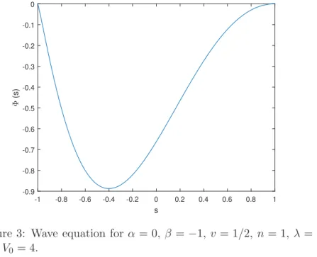
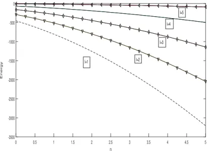
The graph of the wave function Ψn(s) and the energy En are shown in Figures 3 and 4, respectively.

s

-1 -0.8 -0.6 -0.4 -0.2 0 0.2 0.4 0.6 0.8 1

Φ

(s)

-0.9 -0.8 -0.7 -0.6 -0.5 -0.4 -0.3 -0.2 -0.1 0

Figure 3: Wave equation forα = 0, β =₋1, v= 1/2, n= 1, λ= 1 andV0 = 4.

4. Conclusion

n

0 0.5 1 1.5 2 2.5 3 3.5 4 4.5 5

Energy

-3500 -3000 -2500 -2000 -1500 -1000 -500 0

l=1 l=2

l=3 l=4

l=5

Figure 4: Energy En for different values of λ= 1.

References

[1] R.N. Costa Filho, M.P. Almeida, G.A. Farias and J.S. Andrade, Jr., Dis-placement operator for quantum systems with position-dependent mass, Phys. Rev. A,84(2011), 050102(R).

[2] V.D. Dinh, Well-posedness of nonlinear fractional Schr¨odinger and wave equations in Sobolev spaces,Int. J. Appl. Math.,31, No 4 (2018), 483–525; DOI: 10.12732/ijam.v31i4.1.

[3] H. Eleuch, Y.V. Rostovtsev and M.S. Abdalla, Analytical solution for one-dimensional scattering problem,Optics Communications, 284(2011), 5457.

[4] H. Eleuch, Y.V. Rostovtsev and M.O. Scully, New analytical solution of Schr¨odinger equation, Europhys. EPL,89(2010), 50004.

[5] N. Froman and P.O. Froman, JWKB Approximation, AbeBooks, North-Holland, Amsterdam (1965).

[7] P.K. Jha, H. Eleuch and Y.V. Rostovtsev, Analytical solution to position dependent mass Schr¨odinger equation,J. Mod. Optic.,58(2011), 652–656. [8] H.A. Kramers, Wellenmechanik und halbzahlige quantisierung,Z. Physik,

39(1926), 828–840.

[9] H.W. Lee and M.O. Scully, The Wigner phase-space description of collision processes,Found. Phys.,13, No 1 (1983), 61–72.

[10] S.H. Mazharimousavi, Revisiting the displacement operator for quan-tum systems with position-dependent mass, Phys. Rev. A, 85 (2011), 034102(R).

[11] S. Meyur, Position dependent mass for the Hulth´en plus hyperbolic cotan-gent potential, Bulg. J. Phys.,38 (2011), 357–363.

[12] O. Mustafa and S.H. Mazharimousavi, D-dimensional generalization of the point canonical transformation for a quantum particle with position-dependent mass, J. Phys. A,39(2006), 10537–10547.

[13] A.F. Nikiforov and V.B. Uvarov, Special Functions of Mathematical Physics, Birkhauser, Basel (1988).

[14] E. Pozdeeva and A. Schulze-Halberg, Trace formula for Green’s functions of effective mass Schr¨odinger equations and N-th order Darboux transfor-mations,Int. J. Mod. Phys. A,23(2008), 2635–2647.

[15] R. Renan, M.H. Pacheco and A.C.S. Almeida, Treating some solid state problems with the Dirac equation,J. Phys. A,33, No 50 (2000), L509. [16] R.W. Robinet, Quantum Mechanics, Oxford Univ. Press, Oxford (2006).

[17] E.C. Romao, M.D. de Campos and L.F.M. de Moura, Solutions for prob-lems in the finite amplitude wave propagations using the method of char-acteristics, Int. J. Appl. Math.,24, No 3 (2011), 339–347.

[18] B. Sangar´e, A moving mesh method for the nonlinear Schr¨odinger equation, Int. J. Appl. Math.,29, No 1 (2016), 105-126; DOI:10.12732/ijam.v29i1.9. [19] A. Schmidt, Wave-packet revival for the Schr¨odinger equation with

position-dependent mass,Phys. Lett. A,353, No 6 (2006), 459–462. [20] E. Schr¨odinger, Quantisierung als eigenwertproblem,Ann. Phys. (Leipzig),

[21] R. Sever, C. Tezcan, ¨O. Yesiltas and M. Bucurgat, Exact solution of effec-tive mass Schr¨odinger equation for the Hulthen potential, Int. J. Theor. Phys.,47(2008), 2243–2248.

[22] E.L. Shishkina, Inversion of the mixed Riesz hyperbolicB-potentials,Int. J. Appl. Math.,30, No 6 (2017), 487–500, DOI: 10.12732/ijam.v30i6.3. [23] A. Sinha, Scattering states of a particle with position-dependent mass in

a double heterojunction,Europhys. Lett., 96, No 2 (2011), 20008.

[24] A. de Souza Dutra, Ordering ambiguity versus representation,J. Phys. A, 39, No 1 (2005), 203-210.

[25] A. de Souza Dutra and C.A.S. Almeida, Exact solvability of potentials with spatially dependent effective masses,Phys. Lett. A,275 (2000), 25–30. [26] C. Tezcan and R. Sever, A general approach for the exact solution of the

Schr¨odinger equation, Int. J. Theor. Phys.,48(2009), 337–357.