THE SOLUTION OF FREE-FORM DEFORMATION PROBLEM USING PSEUDOINVERSE

Volume 31 No. 6 2018, 833-852

ISSN: 1311-1728 (printed version); ISSN: 1314-8060 (on-line version) doi:http://dx.doi.org/10.12732/ijam.v31i6.12

THE SOLUTION OF FREE-FORM DEFORMATION PROBLEM USING PSEUDOINVERSE

Jana Prochazkova1§, Jiri Novak2 1,2_{Brno University of Technology}

Technicka 2, Brno – 616 69, CZECH REPUBLIC

Abstract: The basis of many commonly used computer graphics algorithms is concealed in well known algebraic structures. Our interest is focused on a method Free Form Deformation (FFD) used in the areas such as surface mod-eling, image registration or animation. The algebraic core can be described by the undetermined system of equations and pseudoinverse or Lagrange mul-tipliers are perfect tools to solve it. Mutual interconnection is not obvious, so we deduce the fundamental theorems and we present FFD method and its application on general B-spline surfaces.

AMS Subject Classification: 93E24, 65F20

Key Words: free-form deformation, least square method, pseudoinverse, B-spline, NURBS, Lagrange multipliers

1. Introduction

of equations (see [31], [1]). We use the pseudoinverse as the computational tool to solve the best results. We also show that this solution corresponds to the Lagrange multipliers (Section 2.3).

Section 2.1 of our article deals with the definition of spline function and spline surfaces. In Section 2.2, we introduce the basic definitions and properties related to the pseudoinverse and the pseudoinverse solution for the linear system of equations. Section 3 covers the main idea of FFD with the proof of the key theorem.

2. Theoretical background 2.1. B-spline

The theory of piecewise polynomial B-spline functions and following B-spline curves and surfaces is well known and precisely described in the literature, e.g. [23], [26]. The main idea is based on the combination of the B-spline basis function with a regular grid of control points and pair of knot vectors. The knot vector is a sequence of numbers provided that each one is greater than or equal to the preceding one. The knot vectors as control points describe the shape of result surface [24]. Knot vectors are generally placed into one of three categories: uniform, open uniform, and non-uniform. The algorithm FFD is independent on the type of knot vector.

In our work, we apply on non-uniform B-spline surfaces. The usage of point weights (B-spline becomes a rational B-spline) only transfers the com-putational problem to homogenous coordinates in projective space [13]. So that we work without the rational extension. The following section provides the brief overview of B-spline basic definitions and the example of the basis B-spline functions is in Figure 1.

Definition 1. Let U = (u0, . . . , um) be a knot vector (ui ≤ ui+1, i = 0, . . . , m−1). Then the i-th B-spline basis function of degree p is defined recurrently as:

Ni,0=

1 if ui ≤u < ui+1 0 otherwise ,

Ni,p(u) =

u−ui

ui+p−ui

Ni,p−1(u) +

ui+p+1−u ui+p+1−ui+1

Figure 1: B-spline basis functions Ni,3(u) and spline functions

Ni,3(u)Nj,3(v).

Definition 2. Let {Pi} be the control points and {wi}, i = 0, . . . , n be

the weights, and theNi,p(u) bep−th degree B-spline basis functions. Then the

NURBS curve is defined as: C(u) =

Pn

i=0Ni,p(u)wiPi Pn

i=0Ni,p(u)wi

. (2)

NURBS surface is defined as a tensor product of NURBS curves. Ev-ery NURBS topology needs the regular k+ 1×l+ 1 control points net Pij,

weights wij, i = 0,1, . . . , k, j = 0,1, . . . , l, knot vectors U = (u0, . . . , um),

V = (v0, . . . , vn) and degrees p, q. Then the NURBS surface can be expressed

as:

S(u, v) =

Pk i=0

Pl

j=0Ni,p(u)Nj,q(v)wijPij Pk

i=0

Pl

j=0Ni,p(u)Nj,q(v)wij

. (3)

If the weights of all points are equal to one, we get a non-uniform B-spline surface and afterwards we can rewrite Eq. (3) as:

S(u, v) =

k X

i=0

l X

j=0

Ni,p(u)Nj,q(v)Pij (4)

and Eq. (2) as a non-uniform B-spline curve:

C(u) =

n X

i=0

Ni,p(u)Pi. (5)

scheme or control point insertion remain preserved. The general idea of T-spline was published by Sederberg [29]. Generally, the arbitrary surface point is com-puted with the combination of the control points and B-spline basis functions, only the knot vectors are not global but connected unambiguously with every control point. The description of this knot vectors is done by T-mesh in (s, t) parameter space. T-mesh often contains T-junctions (similar to letter T). This special type is a vertex which is shared by one s-edge and two t-edges, or by onet-edge and twos-edges.

T-spline surface of degree p is defined by control points Pi, i = 1, . . . , n.

Every point is connected with two knot vectors of length 2p−1 derived from T-mesh and we set degreep= 3. It is also possible to add weights to the control points to make weighted T-spline surface [19].

The mathematical expression of T-spline is:

P(s, t) =

n X

i=1

PiBi3(s, t). (6)

The basis functionsB_i3(s, t) are given by

B_i3(s, t) =N[si0, si1, si2, si3, si4](s)N[ti0, ti1, ti2, ti3, ti4](t).

where N[si0, si1, si2, si3, si4](s) is B-spline basis function associated with the knot vector

si = [si0, si1, si2, si3, si4]

and N[ti0, ti1, ti2, ti3, ti4](t) is associated with the knot vector ti= [ti0, ti1, ti2, ti3, ti4].

2.2. Inverse, pseudoinverse

This section gives the definitions and theorems of pseudoinverse that are essen-tial to subsequent parts (more details in [3]).

Definition 3. LetA ∈ Cm×n _{be a general matrix. We say that A is left}

invertible if there exists an n×m matrix C such that CA = In. We call C

a left inverse of A. We say that A is right invertible if there exists an n×m matrixD such that AD=Im. We call D a right inverse of A. We say that A

Remark 1. Let A ∈ Cm,n _{be a general matrix and} A∗ _{its Hermitian} transpose matrix, then:

r(A∗·A) =r(A·A∗) =r(A). (7) Note thatr is the rank of the matrix [33].

Theorem 4. Let A∈Cm,n_{. The following claims are valid:} 1. A is right (left) invertible,

2. A is full row (column) rank,

3. A·A∗ _{is regular.}

Proof. (1)-(2): LetA be a m×n matrix. Suppose, that (1) holds and B is the right inverse ofA. It holds that A·B =Im. Letm be a rank ofA·B:

m=r(A·B)≤r(A)≤m. (2)-(3): Letr(A) =m and due to Remark 1, we have

r(A·A∗) =r(A) =m and matrixA·A∗ is regular.

(3)-(1): IfA·A∗ is regular, let B =A∗(A·A∗)−1_{. Then A·B =I}

m and

B is right inverse of matrixA.

Definition 5. LetA∈Cm,n_{. The matrixA}+ _{is the pseudoinverse ofAif:}

1. AA+A=A, 2. A+AA+ =A+, 3. (AA+)∗_=AA+_, 4. (A+_A)∗_=A+_A.

Furthermore, the pseudoinverse A+ always exists and is unique. The proof is e.g. in [1], [22].

Theorem 6. LetA∈Cm,n_{,m≥nwith full row rank. The matrixA·A}∗ is regular and invertible and the pseudoinverse of A is:

Proof. Suppose that the matrix A ism×n, wherem < nand A is full row rank. Due to Remark 1, we get m = r(A) = r(A·A∗) and consequently the matrixA·A∗ is regular. Let

X=A∗·(A·A∗)−1.

Then A·X =A·A∗·(A·A∗)−1 =Im. The Penrose conditions (1)-(3) holds.

The condition (4) can be proved by:

(X·A)∗ =A∗·X∗=A∗· (A·A∗)−1∗·A= =A∗·((A·A∗)∗)−1·A=A∗·(A·A∗)−1·A=X·A.

Analogously, this theorem can be formulated for full column rank matrices. Remark 2. If A∈Rm,n_{, the Theorem 6 can be rewritten as:}

A+=AT · AT ·A−1. (9) 2.2.1. Pseudoinverse solution for linear system of equations We define Hermitian inner product and the norm of the vectorXin this section. Generally, we work in complex domain but we need only real domain for the application in FFD.

Definition 7. Let X, Y ∈Cn

X =      x1 x2 .. . xn     

, Y =

     y1 y2 .. . yn      .

We define the Hermitian inner product as

(X, Y) =Y⋆·X=

n X

i=1

xi·yi (10)

and the norm of the vector X is defined as:

kXk=pX, X =

v u u t n X i=1

xi·xi = v u u t n X i=1

Definition 8. We say that two vectors X, Y are orthogonal if (X, Y) = 0. We can write

X⊥Y.

Theorem 9(Pythagorean theorem for vectors). For orthogonaln-dimensional vectors X, Y we have:

kX+Yk2=kXk2+kYk2. (12)

The proof is done by simple equivalent operations of expressionkX+Yk2_.

Theorem 10. Let A ∈ Cm,n_{, P = A·A}+_{, Q = A}+_{·A, X, Y are n} -dimensional vectors in Cn_{. It holds:}

(a) kA·X+ (Im−P)·Yk2=kA·Xk2+k(Im−P)·Yk2,

(b) kA·Y + (Im−Q)·Xk2 =kA·Yk2+k(Im−Q)·Xk2.

Proof. LetR=A·X andS = (Im−P)·Y arem-dimensional vectors and

we can write:

(R, S) = (A·X,(Im−P)·Y) = ((Im−P)·Y)⋆·A·X

=Y⋆·(Im−P)·A·X=Y⋆·A·X−Y⋆·A·A+·A·X

=Y⋆·A·X−Y⋆·A·X= 0.

The vectors R, S are orthogonal and the theorem holds due to Pythagorean theorem for vectors. Statement (b) can be proved analogously.

The system of linear equations is given by

A·X=B, (13) where

A=



 

a₁₁ · · · a₁n

.. .

am1 · · · amn 

 

and X=





x1

xn 

B = 



b1

bm 

The following Theorem 11 explains the least squares solution to the system (13) with minimum norm [7]. This solution is X0, given by the expression:

X0=A+·B. (14)

Theorem 11. LetX∈Cn_,X 6=X₀ ben-dimensional vector, then we get

kA·X0−Bk ≤ kA·X−Bk. (15)

In casekA·X₀−Bk ≤ kA·X−Bkit holds

kX₀k<kXk. (16)

Proof. The proof is based on rewriting of Theorem 10. A proof based on ortogonality is in [1].

2.3. Lagrange problem

Let A·X = B be a general linear system of m equations with n unknowns where n > m (undetermined system) and aij, xjbj ∈ R, i = 1, . . . , m, j =

1, . . . , n. Generally, according to the Rouch-Capelli theorem, the rank in an undetermined system is necessarily less than the number of unknowns, there are undoubtedly an infinitude of solutions.

Nevertheless, we want to minimize the normkXkunder the system of con-straintsAX=B. We introduce a vectorλof Lagrange multipliers and consider the function

L=XTX−λT(AX−B). (17)

The solution using derivatives for all variables xi and λgives the system (18),

(19):

2XT _−λT_{A=o (18)}

−(AX−B) =o. (19)

After doing some simplifications of Eq. (18), we get:

X = 1 2A

T_{λ. (20)}

Substituting Eq. (20) to Eq. (19) we get: 1

2AA

Suppose that the matrix A is full row rank so that the matrix AAT _due

to Theorem 4 is regular matrix and the inverse exists. The Eq. (21) can be rewritten as follows:

(AAT)−1AATλ = 2(AAT)−1B

λ = 2(AAT)−1B. (22) Substituting Eq. (22) to Eq. (20) and using Remark 2 we can write:

X = 1 22A

T_(AAT₎−1

| {z }

A+ B

X = A+B. (23) Here we can clearly see the relation between pseudoinverse and the solution based on minimization.

3. FFD theory and computation

The FFD method was firstly published by Sederberg and Perry in the year 1986. The principle is based on the insertion of the solid representation to the regular parallelpiped; subsequent transformation recomputes the position of the solid points with respect to the modified points of the lattice [28].

The computation is based on the tensor product trivariate Bernstein poly-nomial. Every object pointX has (s, t, u) coordinates in the coordinate system on a parallelpiped region:

X=X0+sS+tT+uU. (24)

Let Pijk, i = 0, . . . , l, j = 0, . . . , m, k = 0, . . . , n are control points on a

lattice. The deformation is represented by a movement of the control points Pijk from their latticial positions. New position of point Xnew is computed by:

Xnew= (25)

= l X i=0 l i !

(1−s) l−i si "m X j=0 m j !

(1−t) m−j tj n X k=0 n k !

(1−u) n−k

ukPijk

!#

,

where (s, t, u) are parameters in Eq. eqrefeq:1.

the other FFD types. The limitation for the rectangular shape of the control lat-tice is eliminated for example by the usage of Dirichlet surfaces (defined in [9]). The authors in [21] introduce the Dirichlet FFD (or DFFD) that works with so-called Sibson coordinates that describe arbitrary location inside the convex hull of the point set as a linear combination of its Delaunay neighbors in the set. Point-based (PB) FFD [20] uses ellipsoidal radial basis function to define the deformation space. This approach does not need Delaunay triangulation as the DFFD.

Another solution to overcoming the rectangular topology limitation of tensor-product volumes is based on subdivision surfaces. The authors in [10] claim that it is the bridge between the discrete control mesh and the smooth surface. The pioneering method was proposed in [6]. The CatmullClark subdivision volume [4] is used as the intermediate deformation space and it guarantees that the topology of the control lattice can be arbitrary. It makes the deformation more flexible. Since the subdivision volume is defined by the recursive refine-ment rules, the refinerefine-ment procedure convergence is problematic and thus the smoothness of the deformation space is not guaranteed. Furthermore, control lattice generation is not easy and the storage and computational costs are high. The method [10] brings low storage and computational costs and more intuitive and simpler control. It presents the construction of subdivision surface defined by control mesh spans. The object is embedded into space by the nearest point rule. The object shape is changed accordingly to the change of the shape of the control mesh. The computational and storage cost are between O(n2) and O(n3_).

An extension of subdivision surface usage with a path of deformation and an influence area constraints is described in [17]. The main advantage of this method is that it uses only vertices of an object and satisfies the geometrical constraints provided by the user.

The subdivision scheme uses only regular control lattice that covers the object. There is a possibility to employ irregular subdivision T-lattice that is based on T-splines [29, 19]. The authors in [32] proposed a two-stage algo-rithm that generates the multiresolution lattices for weighted T-spline volumes and processes the local or global deformation for arbitrary shape by combin-ing weights change and lattice manipulation. However, this method has some limitation that is based on the irregular lattice, e.g. it cannot operate one row of the control lattice in some directions and the computational costs are also higher.

costs, simplicity, independence of object representation. It is very difficult to find a deformation method to satisfy all of these criteria. It is important to note that from the user point-of-view, it does not matter if the transformed object is 3-dimensional, embedded with subdivision surface or a parametric surface, the user always uses the same process to model a complex object: load an initial object from a library and deform it via FFD methods to follow his demand needs [25].

Direct movement of the surface points is the next level of FFD controlling. The main idea is the direct shift of the surface points and the control net points are recomputed automatically. The users no longer need to understand the tensor-product Bezier surfaces or NURBS to use the FFD for modeling. This method satisfies most of the conditions: it is intuitive, versatile, simple to shape modification, it needs low memory and the computation is fast.

The process of direct manipulation was firstly described in [15]. It employs a pseudo-inverse (generalized inverse) matrix that as [16] mentioned involves complicated calculations. The authors in [16] suggests the approach based on a constrained optimization without the need of pseudoinverse computation. These two approaches are very different at first sight but they describe the same problem. In the following sections, we try to investigate mutual intercon-nection of these two solutions. We put emphases on the comprehension and detailed description of these two methods to formulate suitable apparatus for the following computer processing.

The problem of FFD is well known but it still offers the up to date appli-cations in many areas, most in car, ships or aircraft manufacturing and also in design. For example, [5, 14, 2] reconnect the main idea of Sederberg’s FFD manipulation with suitable apparatus like ICP algorithm or subdivision sur-faces for smart ship hull constructions. An interesting design application is a non-realistic modeling where two 3D geometric models are merged to preserve a shape silhouette from different views [27, 30].

3.1. Free Form Deformation

Without loss of generality we suppose that the degree of the spline curves and surfaces is p = q = 3. The generalization for arbitrary degree is possible but the curves and surfaces are often in cubic form.

surface can be expressed as:

Qij(u, v) = k X

i=0

l X

j=0

Ni,3(u)Nj,3(v)Pij. (26)

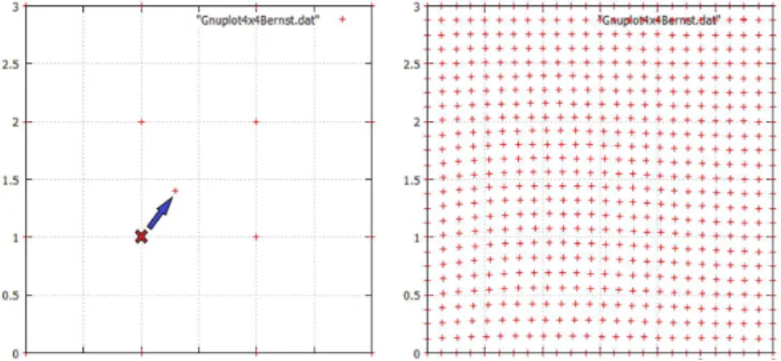
We setk, l= 3 because of the local control property of B-spline functions. The movement of one point affects only (p+ 1)×(q+ 1) control points, p=q= 3 so that we recompute 4×4 control points (Fig. 2, left). Then, we can rewrite Eq.(26) as:

Qij(u, v) =

3

X

i=0 3

X

j=0

Ni,3(u)Nj,3(v)Pij, (27)

or symbolically

Q=NP, (28)

whereN is a row vector (matrix 1×16):

N= (Nk)16_k=0 where N4i+j+1=Ni(u)Nj(v),

i, j= 0, . . . ,3,

and P is a 16×3 matrix that contains the x, y, z−coordinates of the control points,

P= (P_ijx, P_ijy, P_ijz,)3_i,j=0.

Figure 2: Affected control point net 4×4 in the case of surface point Qmovement (left), FFD transformation on the cylinder (right).

Theorem 12. Let Qs be a source point and Qt be a target point.

Sim-ilarly, the Ps denotes the source control net of points and Pt is the matrix of

transformed points. Result displacement ∆Pof the control points Pt is equal

to:

∆P=N+·∆Q (29)

where∆Q=Qt−Qs,∆P=Pt−Ps.

Proof. We can write the coordinates of the source and target pointQs,Qt

as:

Qs=NPs, (30)

Qt=NPt. (31)

We know that ∆Q=Qt−Qs and ∆P=Pt−Ps. The difference Eq. (30) −

Eq. (31)can be written as:

∆Q=N∆P. (32)

We use the scheme of optimization described in Section 2.3 and we get the solution

∆P=N+·∆Q. (33)

Remark 3. The computation of N+ _{is specific so that we mention the} detailed construction here. The matrix N∈R1,16 _{and its pseudoinverse N}+₌

NT _{is 16×1. It follows that NN}T _{is only a real number and corresponds to}

the dot product. It is clearly visible that (NNT)−1 = _P161

k=1Nk2

(34)

and the pseudoinverseN+ can be computed as: N+= _P161

k=1Nk2

NT∆Q (35)

and the displacement of the control points Pare:

∆P= _PN₁₆i∆Q

k=1Nk2 !16

i=1

(36)

= Ni∆Q

x

P16

k=1Nk2

, Ni∆Q

y

P16

k=1Nk2

, Ni∆Q

z

P16

k=1Nk2 !16

Remark 4. The Eq. (36) is often used in the programming applications. Figures 3 and 4 show the planar and surface application of FFD technique.

Figure 3: Single transformation of regular control net and resulting surface.

Figure 4: General surface point movement (left) and resulting trans-formation of control point net (right).

The interesting question is one-to-one property between original and trans-formed spline surface. Theorem 13 was firstly presented in Goodman [12]. The condition gives the system of 3m(m+ 1) + 2n(n+ 1) linear inequations, so that the computation time increases rapidly with higher number of control points. We have to note that the condition is sufficient not necessary.

Theorem 13. The function given in(27) is one-to-one if|∆P|∞≤0.48.

Proof. The proof is in [18].

dragged beyond their volume of the influence, it sometimes generates wild hy-perpatch distortion. Using the subsequent small injective deformations [11] prevents the self-intersections. The article presents a set of theoretical condi-tions based on Jacobian of FFD and its evaluacondi-tions and weak condition using conic-hull hodograph test.

Remark 5. NURBS surface FFD works with the same apparatus as spline surfaces. We only use the homogeneous coordinates to attach the point weights. LetQT _{= Q}T

x,QTy,QTz,QTw

be the target point andQS _{= Q}S

x,QSy,QSz,QSw

be a source point. The difference vector is ∆Q=QT_−QS_{= Q}X_,QY_,QZ_,QW_.

We can rewrite Eq. (36) as:

∆P= _PN₁₆i∆Q

k=1Nk2 !16

i=1

(37)

= Ni∆Q

x

P16

k=1Nk2

, Ni∆Q

y

P16

k=1Nk2

, Ni∆Q

z

P16

k=1Nk2

, Ni∆Q

w

P16

k=1Nk2 !16

i=1

=





Ni∆Qx

P16 k=1N

2 k Ni∆Qw

P16 k=1N

2 k

,

Ni∆Qy

P16 k=1N

2 k Ni∆Qw

P16 k=1N

2 k

,

Ni∆Qz

P16 k=1N

2 k Ni∆Qw

P16 k=1N

2 k ,1   16 i=1 .

3.2. Multiple point constraints

Suppose that we get a set of h point constraints and we search for the final displacement of the control points. The solution is clearly described in following theorem.

Theorem 14. A direct manipulation of FFD withhpoint constraints can be decomposed into h manipulations with single point constraints.

Proof. LetQ1

s, . . . ,Qhs are source points andQ1t, . . . ,Qht are corresponding

target points. The proof is based on the decomposition of the shift vectors ∆Ql = ∆Qlt−∆Qls to the sequence: ∆(l)Ql, wherel= 1, . . . , h. We compute

the values of the control point displacement ∆(l)_{Pin one step as in Eq. (36):}

∆(l)P= Ni∆ (l)_Q

P16

k=1Nk2 !16

i=1

The global displacement of the control points P is the sum of the previous partial transformation.

∆P=

h X

l=1

Ni∆(l)Q P16

k=1Nk2 !16

i=1

. (39)

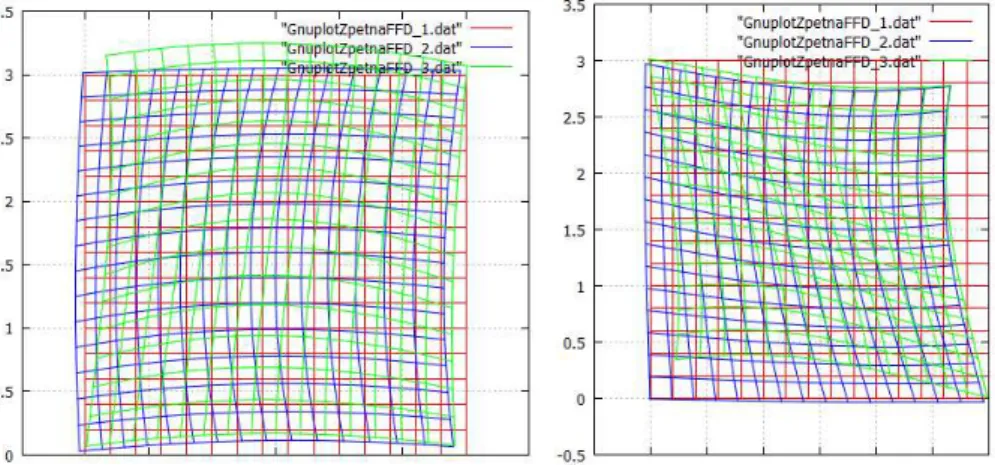
The illustration of FFD transformation with two subsequent point con-straints is in Figure 5. We make subsequent transformations of two arbitrary point of spline surface: red graph is initial control net, blue graph is first de-formation, green graph is second deformation.

Figure 5: Multiple point constraints: red graph is initial control net, blue graph is first deformation, green graph is second deformation.

4. Conclusion

We describe multiple point constraints problem as the composition of single point constraints in Section 3.2.

It is also possible to work with rational splines – NURBS (Section 2.1) by adding the weights to control points. The weight means the influence of given point to the resulting shape of the surface. The presented FFD theorem holds, only the homogeneous coordinates (in projective space) should be used instead of Euclidean ones.

References

[1] J.C.A. Barata, M.S. Hussein, The Moore–Penrose pseudoinverse: A tuto-rial review of the theory, Brazilian Journal of Physics, 42, No 1 (2012), 146–165.

[2] R. Bearee, J.Y. Dieulot, P. Rabate, An innovative subdivision-ICP regis-tation method for tool-path correction applied to deformed aircraft parts machining,International Journal of Advanced Manufacturing Technology, 53(2011), 463–471.

[3] A. Ben-Israel, T.N.E. Greville, Generalized Inverses, Theory and Applica-tions, Springer-Verlag, New York, Second Edition (2003).

[4] E. Catmull, J. Clark, Recursively generated B-spline surfaces on arbitrary topological meshes,Computer Aided Design,9, No 6 (1978), 183–188. [5] A. Coppede, G. Vernengo, D. Villa, A combined approach based on

Subdi-vision Surface and Free Form Deformation for smart ship hull form design and variation, Ships and Offshore Structures (2018), 769–778.

[6] R. MacCracken, Kenneth I. Joy, Free-form deformations with lattices of arbitrary topology, In: Proc. of the 23rd Annual Conference on Computer Graphics and Interactive Techniques (SIGGRAPH ’96), ACM, New York (1996), 181–188.

[7] P.J. Davis, Circulant Matrices, John Wiley and Sons Inc., New York, Second Edition (1994).

[9] G. Farin, Surface over Dirichlet tessellations, Geometric Aided Design, 7 (1990), 281–292.

[10] J. Feng, J. Shao, X.Jin, Q. Peng, A.R. Forrest, Multiresolution free-form deformation with subdivision surface of arbitrary topology, Visual Com-puter,22, No 1 (2006), 28–42.

[11] J.E. Gain, N.A. Dodgson, Preventing self-intersection under free-form de-formation, IEEE Transactions on Visualization and Computer Graphics, 7, No 4 (2001), 289–298.

[12] T.N.T. Goodman, K. Unsworth, Injective bivariate maps, Annals of Nu-merical Mathematics,3 (1996), 91-104.

[13] A. Holme, Projective Space, Geometry: Our Cultural Heritage, Springer, Berlin Heidelberg (2002), 221–232.

[14] J. Hradil,Adaptive Parameterization for Aerodynamic Shape Optimization in Aeronautical Applications, Brno University of Technology, Faculty of Mechanical Engineering, Institute of Aerospace Engineering, Brno (2015). [15] W.M. Hsu, J.F. Hughes, H. Kaufman, Direct manipulation of Free-Form Deformations, In: ACM SIGGRAPH Computer Graphics,26, No 2 (1994), 177–184.

[16] S.M. Hu, H. Zhang, C.L Tai, et al., Direct manipulation of FFD: effi-cient explicit solutions and decomposible multiple point constraints,Visual Computer,17, No 6 (2001), 370–379.

[17] S. Lanquetin, R. Raffin, M. Neveu, Curvilinear constraints for free form de-formations on subdivision surfaces,Mathematical and Computer Modeling, 51, No 34 (2010), 189–199.

[18] S. Lee, G. Woberg, K.-Y. Chwa, S.Y. Shin, Image metamorphosis with scattered feature constraints, IEEE Transactions on Visualization and Computer Graphics,2, No 4 (1996), 337–354.

[19] L. Liu, Y.J. Zhang, X. Wei, Weighted T-splines with application in repa-rameterizing trimmed NURBS surfaces, Computer Methods in Applied Mechanics and Engineering,295 (2015), 108–126.

[21] L. Moccozet, N.M. Thalmann, Dirichlet Free-Form deformations and their application to hand simulation. In: Proc. of the Computer Animation (CA 97), IEEE Computer Society, Washington, DC (1997), 93–102.

[22] R. Penrose, A generalized inverse for matrices, Mathematical Proc. of the Cambridge Philosophical Society,51, No 3 (1955), 406–413.

[23] L. Piegl, W. Tiller, NURBS Book, Springer-Verlag, Berlin Heidelberg (1997).

[24] J. Prochazkova, D. Prochazka,An Influence of Knot Vectors on the Shape of NURBS Surfaces, VUT Brno (2007), 95–96.

[25] R. Raffin, Free form deformations or deformations non-constrained by ge-ometries or topologies, Lecture Notes in Computational Vision and Biome-chanics,7 (2013), 49–74.

[26] D. Rogers, An Introduction to NURBS, Morgan-Kaufmann, Burlington (2000).

[27] J. Snchez-Reyes, J.M. Chacn, Anamorphic Free-Form deformation, Com-puter Aided Geom. Des.,46(2016), 30–42.

[28] T.W. Sederberg, S.R. Parry, Free-form deformation of solid geometric mod-els. In: Proc. of the 13th Annual Conference on Computer Graphics and Interactive Techniques (SIGGRAPH ’86), ACM, New York (1986), 151– 160.

[29] T.W. Sederberg, J. Zheng, A. Bakenov, A. Nasri, T-splines and T– NURCCS, ACM Transactions on Graphics,22, No 3 (2003), 477–483. [30] G. Sela, G. Elber, Generation of view dependent models using free form

deformation, The Visual Computer,23, No 3 (2007), 219–229.

[31] I.R. Shafarevich, A. Remizov, Linear Algebra and Geometry, Springer-Verlag, Berlin Heidelberg (2012).

[32] W. Song, X. Yang, Free-form deformation with weighted T-spline, Vis. Comput., 21(2005), 139–151.

[34] N.J. Tustison, B.B. Avants, J.C. Gee, Directly manipulated Free-Form de-formation image registration, In: IEEE Transactions on Image Processing, 18, No 3 (2009), 624–635.

[35] R. Van De Walle, H.H. Barrett, K.J. Myers, M.I. Aitbach, B. Desplanques, A.F. Gmitro, J. Cornelis, I. Lemahieu, Reconstruction of MR images from data acquired on a general nonregular grid by pseudoinverse calculation,