An Ensemble Method for Large Scale Machine Learning
with Hadoop MapReduce
by
Xuan Liu
Thesis submitted to the
Faculty of Graduate and Postdoctoral Studies In partial fulfillment of the requirements For the degree of Masters of Applied Science in
Electrical and Computer Engineering
Ottawa-Carleton Institute for Electrical and Computer Engineering School of Electrical Engineering and Computer Science
University of Ottawa
Table of Content
List of Figures ... v
List of Tables ... vi
List of Abbreviations ... vii
Abstract ... viii Acknowledgements ... ix Chapter 1 ... 1 Introduction ... 1 1.1 Motivation ... 2 1.2 Thesis Contributions ... 6 1.3 Thesis Outline ... 8 Chapter 2 ... 9 Background ... 9 2.1 Ensemble Learning ... 10
2.1.1 Reasons to Choose Ensemble Methods ... 12
2.1.2 Reasons for Constructing Ensembles ... 13
2.1.3 Ensemble Diversity ... 16
2.1.4 Methods to Build Base Classifiers ... 20
2.1.5 Methods to Combine Base Classifiers ... 21
2.1.7 Meta-learning Algorithm ... 29
2.2 Large Scale Machine Learning ... 34
2.2.1 Large Scale Datasets ... 35
2.2.2 Hadoop ... 37
2.2.3 MapReduce ... 38
2.2.4 Hadoop Distributed File System (HDFS) ... 48
2.2.5 Related Work ... 52 2.3 Conclusion ... 56 Chapter 3 ... 58 Meta-boosting Algorithm ... 58 3.1 Introduction ... 58 3.2 Proposed Method ... 60
3.2.1 Combining AdaBoost Using Meta-learning ... 60
3.2.2 Detailed Procedures and Algorithm ... 62
3.2.3 Advantages of Our Algorithm ... 68
3.3 Experimental Setup and Results ... 70
3.3.1 Comparison Between Meta-boosting and Base Learners ... 72
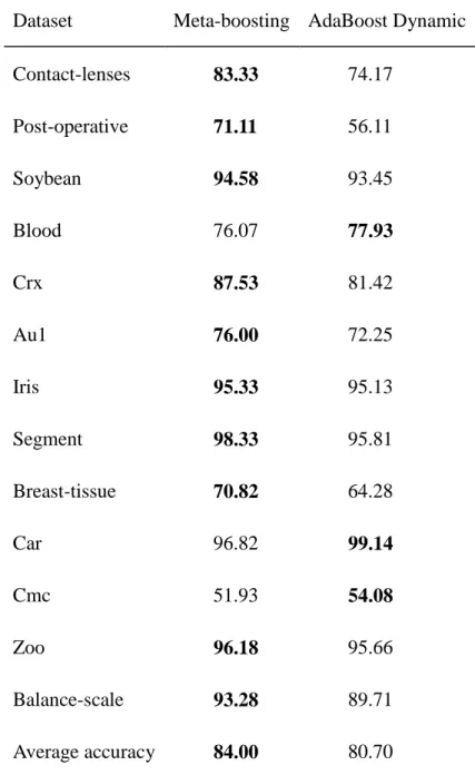
3.3.2 Comparison Between Meta-boosting and AdaBoost Dynamic ... 75
3.4 Discussion ... 75
3.5 Conclusions ... 78
Chapter 4 ... 79
4.1 Introduction ... 79
4.2 Related Work ... 82
4.3 Framework ... 85
4.4 Experiments ... 91
4.4.1 Parallel Adaboost Algorithm (Adaboost.PL) ... 91
4.4.2 Experiment Settings ... 93
4.4.3 Performance Results ... 94
4.5 Conclusions ... 99
Chapter 5 ... 100
Conclusions and Future Work ... 100
5.1 Thesis Outcomes ... 100
5.2 Conclusions ... 100
5.3 Future Work ... 103
Reference ... 105
List of Figures
Fig.2.1. A schematic view of ensemble learning ... 10
Fig.2.2.The statistical reason for combining classifiers. ... 14
Fig.2.3.The computational reason for combining classifiers. ... 15
Fig.2.4. The representational reason for combining classifiers... 15
Fig.2.5. AdaBoost.M1 training process ... 28
Fig.2.6. Meta-learning training process for fold j ... 32
Fig.2.7. Work flow of MapReduce framework ... 42
Fig.2.8. A word count example with MapReduce ... 45
Fig.2.9. Information stored in namenode and datanodes. ... 50
Fig.2.10. Client reads data from datanodes through HDFS ... 51
Fig.3.1. The model of Meta-boosting algorithm ... 62
Fig.3.2. Data preparation procedure. ... 63
Fig.3.3. Implementation process for one time training, validation & test. ... 65
List of Tables
Table 2.1. AdaBoost.M1 Algorithm ... 26
Table 2.2. Meta-learning algorithm for training process ... 33
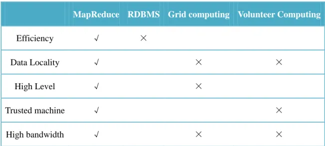
Table 2.3. Comparisons between MapReduce and other systems... 48
Table 3.1. Pseudo code for Meta-boosting algorithm ... 65
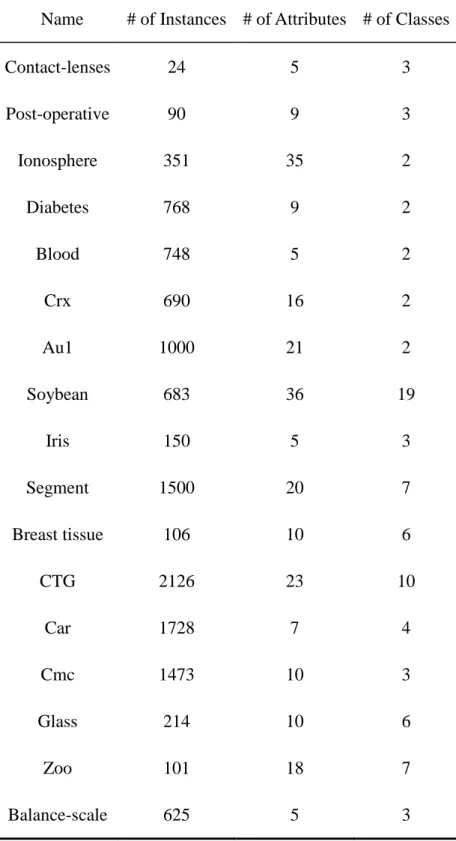
Table 3.2. Datasets used in the experiments... 71
Table 3.3. The accuracy of all the base learners and meta-boosting ... 73
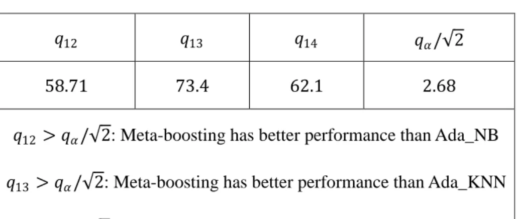
Table 3.4. Friedman‘s test results ... 74
Table 3.5. Nemenyi‘s post-hoc test ... 74
Table 3.6. Comparisons between Meta-boosting and AdaBoost Dynamic ... 76
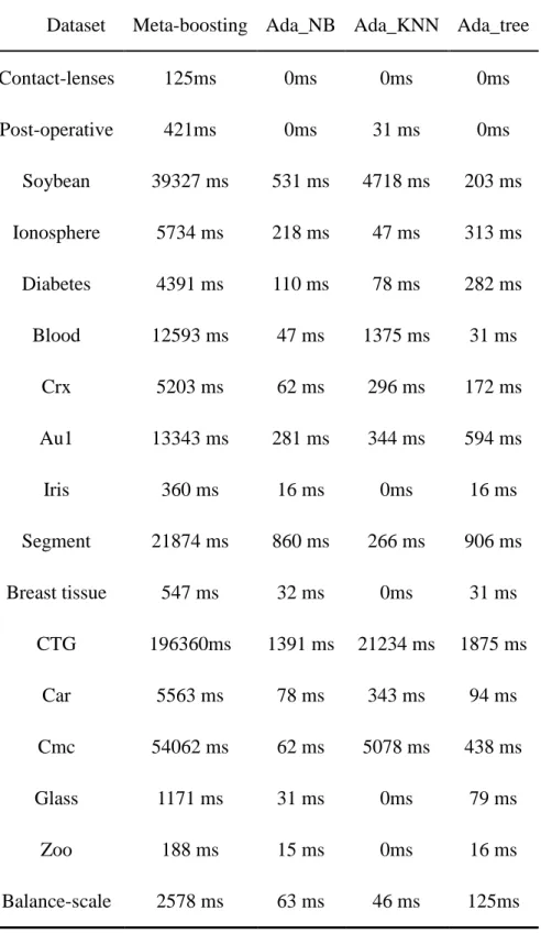
Table 3.7. Computation complexity comparison ( ―ms‖: milliseconds). ... 77
Table 4.1. Algorithm 1: PML Training. ... 86
Table 4.2. Algorithm 2: PML Validation ... 88
Table 4.3. Algorithm 3: PML Test ... 89
Table 4.4. Pseudo code for Adaboost.PL ... 92
Table 4.5. Datasets used in our experiments ... 94
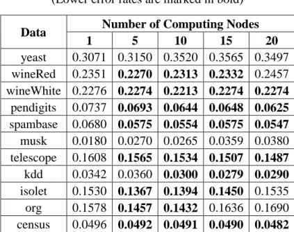
Table 4.6. Error rates for different number of nodes ... 95
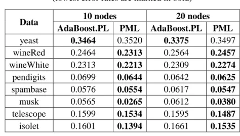
Table 4.7. Comparison of error rates with Adaboost.PL ... 96
List of Abbreviations
API: Application Program Interface CUDA: Unified Device Architecture DSL: Domain Specific Language EM: Expectation Maximization GFS: Google File System
GPU: Graphics Processing Units HDFS: Hadoop Distributed File System HPC: High Performance Computing ML: Machine Learning
MLR: Multi-response Linear Regression MPI: Message Passing Interface
NFL: No Free Lunch
PML: Parallelized-Meta-Learning
POSIX: Portable Operating System Interface PSP: Protein Structure Prediction
RDBMS: Relational Database Management System RDDs: Resilient Distributed Datasets
Abstract
We propose a new ensemble algorithm: the meta-boosting algorithm. This algorithm enables the original Adaboost algorithm to improve the decisions made by different WeakLearners utilizing the meta-learning approach. Better accuracy results are achieved since this algorithm reduces both bias and variance. However, higher accuracy also brings higher computational complexity, especially on big data. We then propose the parallelized meta-boosting algorithm: Parallelized-Meta-Learning (PML) using the MapReduce programming paradigm on Hadoop. The experimental results on the Amazon EC2 cloud computing infrastructure show that PML reduces the computation complexity enormously while retaining lower error rates than the results on a single computer. As we know MapReduce has its inherent weakness that it cannot directly support iterations in an algorithm, our approach is a win-win method, since it not only overcomes this weakness, but also secures good accuracy performance. The comparison between this approach and a contemporary algorithm AdaBoost.PL is also performed.
Acknowledgements
It is my pleasure to take this opportunity to thank all the people who have helped me over the past two years.
I would like to thank my supervisors: Prof. Nathalie Japkowicz and Prof. Stan Matwin who have given me the opportunity to be a member of the TAMALE group at the University of Ottawa. Their passion in research and the critical thinking guided me through my master‘s study. This thesis would be impossible without their constant support and discussions.
Finally, I must thank my family. Their encouragement, understanding and constant love made this work possible.
Chapter 1
Introduction
The supervised learning problem can be described as: given a set of training examples 𝑋1, 𝑦1 , … 𝑋𝑛, 𝑦𝑛 , a learning program will be trained on these training
examples to generate a function 𝑦 = (𝑋). Here 𝑋𝑖 represents a vector of features, 𝑦𝑖 is its label and, in the case of classification, it belongs to a discrete set of classes
1, … , 𝐾 . represents the hypothesis that estimates the true function ∅ which is unknown. It is also called a classifier. In the test process, a new example without label 𝑋′ will be tested on the generated function to obtain its predicted label 𝑦′.
In this scenario, ensemble learning is interpreted as combining the individual decisions of an ensemble of classifiers to classify new examples. It is also known as a multiple classifier system, a committee of classifiers, or a mixture of experts.
Although ensemble-based systems have been put to practice only recently by the computational intelligence community, ensemble-based decision making has been part of our daily lives perhaps as long as the civilized communities existed. In matters of making important decisions about financial, medical, social, or other implications, we often seek many opinions and combine them through some thought process to reach a final decision which is regarded as the most reasonable and wisest one. There are many such examples: consulting several doctors before undergoing major surgery; reading user reviews before
purchasing a product; talking to referees before hiring a potential job applicant; voting to elect a candidate official or decide on a new law; sentencing based on a jury of peers or a panel of judges; even peer reviewing of this thesis.
On the other hand, we have entered the big data age. Here is one proof: the size of the ―digital universe‖ was estimated to be 0.18 zettabytes in 2006 and 1.8 zettabytes in 2011 [1]. A zettabyte is 270 bytes.It is becoming more and more important to organize and
utilize the massive amounts of data currently being generated. Therefore, developing methods to store and analyze these new data has become a very urgent task. One common and popular approach to big data is the cloud computing environment, and its most popular open-source implementation: Hadoop [12]. At the same time, extracting knowledge from massive data sets has attracted tremendous interest in the data mining community.
This thesis develops a new ensemble classification method and adapts it to the big data age. The reminder of this chapter gives the motivations and contributions of the thesis. Section 1.1 presents our motivation for doing this research, while section 1.2 and 1.3provide this thesis‘s contribution and outline, respectively.
1.1 Motivation
One of the main pursuits when designing machine learning algorithms is to gain high accuracy and one of the methods to achieve this goal is to use ensemble learning. Ensemble learning is designed to improve the accuracy of an automated decision-making
system. It has been demonstrated in numerous empirical and theoretical studies that ensemble models often attain higher accuracy than its individual models. This does not necessarily mean that ensemble systems always beat the performance of the best individual classifiers in the ensemble. However, the risk of choosing a poorly behaved classifier is certainly reduced.
Studying methods to construct good ensembles of classifiers has been one of the most active and popular areas of research. To construct an ensemble system: first, a set of base classifiers needs to be generated; second, a strategy is needed to combine these base classifiers. When building base classifiers, we need to select a strategy to make them as diverse as possible. When combining them, a preferred strategy aims to amplify correct decisions and cancel incorrect ones.
The significant development of Machine Learning (ML) in the last few decades has been making this field increasingly applicable to the real world. These applications include business, social media analytics, web-search, computational advertising, recommender systems, mobile sensors, genomic sequencing and astronomy. For instance, at supermarkets, promotions can be recommended to customers through their historic purchase record; for credit card companies, anomaly use of credit cards could be quickly identified by analyzing billions of transactions; for insurance companies, possible frauds could be flagged for claims.
Subsequently, an explosion of abundant data has been generated in these applications due to the following reasons: the potential value of data-driven approaches to optimize every aspect of an organization‘s operation has been recognized; the utilization
of data from hypothesis formulation to theory validation in scientific disciplines is ubiquitous; the rapid growth of the World Wide Web and the enormous amount of data it has produced; the increasing capabilities for data collection. For example, Facebook has more than one billion people active as per Oct 4, 2012, which has increased by about 155 million users as compared to Nov 6, 20111; until May, 2011, YouTube had more than 48
hours of video uploaded to its site every minute, which is over twice the figures of 20102.
These enormous amounts of data are often out of the capacity of individual disks and too massive to be processed with a single CPU. Therefore, there is a growing need for scalable systems which enable modern ML algorithms to process large datasets. This will also make ML algorithms more applicable to real world applications. One of the options is to use low level programming frameworks such as OpenMP [2] or MPI [3] to implement ML algorithms. However, this task can be very challenging as the programmer has to address complex issues such as communication, synchronization, race conditions and deadlocks. Some previous attempts for scalable ML algorithms were realized on specialized hardware/parallel architectures through hand-tuned implementations [4] or by parallelizing individual learning algorithms on a cluster of machines [5] [6] [7].
In very recent years, a parallelization framework was provided by Google‘s MapReduce framework [8] and was built on top of the distributed Google File System (GFS) [ 9 ]. This framework has the advantages of ease of use, scalability and fault-tolerance. MapReduce is a generic parallel programming model, which has become very popular and made it possible to implement scalable Machine Learning algorithms
1https://newsroom.fb.com/Timeline
easily. The implementations are accomplished on a variety of MapReduce architectures [10] [11] [12] and includes multicore [13], proprietary [14] [15] [16] and open source [17] architectures.
As an open-source attempt to reproduce Google‘s implementation, the Hadoop project [12] was developed following the success at Google. This project is hosted as a sub-project of the Apache Software Foundation‘s Lucene search engine library. Corresponding to GFS which is used by Google‘s large scale cluster infrastructure, Hadoop also has its own distributed file system known as the Hadoop Distributed File System (HDFS).
The Map-Reduce paradigm and its implementations are therefore an interesting environment in which to perform ensemble-based Machine Learning. In addition to generating more accurate decision-making systems, ensemble systems are also preferred when the data volume is too large to be handled by a single classifier. This is realized by letting each classifier process a partition of the data and then combining their results. Our thesis is motivated by both of these aspects of ensemble learning: the generation of more accurate ensemble learning models and the handling of enormous amount of data. Even for medium sized data, the approach of parallelizing ensemble learning would be beneficial. The reason is that ensemble learning increases the classification accuracy at the expense of increased complexity.
1.2 Thesis Contributions
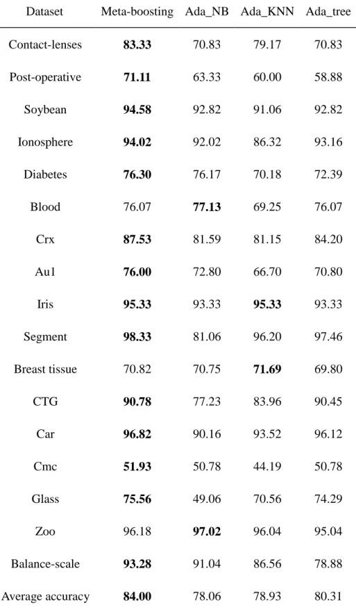
We propose a new ensemble learning algorithm: meta-boosting. Using the boosting method, a weak learner can be converted into a strong learner by changing the weight distribution of the training examples. It is often regarded as a method for decreasing both the bias (the accuracy of this classifier) and variance (the precision of the classifier when trained on different training sets) although it mainly reduces variance. Meta-learning has the advantage of coalescing the results of multiple learners to improve accuracy, which is a bias reduction method. By combining boosting algorithms with different weak learners using the meta-learning scheme, both of the bias and variance are reduced. Moreover, this configuration is particularly conducive for parallelizing general machine learning algorithms. Our experiments demonstrate that this meta-boosting algorithm not only displays superior performance than the best results of the base-learners, but that it also surpasses other recent algorithms.
The accuracy results of the meta-boosting algorithm are very promising. However, one of the issues facing not only this algorithm but also other ensemble learning approaches is that the computation complexity would be huge when confronted with big datasets. Therefore, we plan to apply the relatively simple programming interface of MapReduce to help solve these algorithms‘ scalability problems. However, this MapReduce framework suffers from an obvious weakness: it does not support iterations. This makes those algorithms requiring iterations (e.g. Adaboost) difficult to fully explore
the efficiency of MapReduce. In order to overcome this weakness and improve these algorithms‘s scalability to big datasets, we propose to apply Meta-learning programmed with MapReduce to realize the parallelization. This framework can also be extended to any algorithms which have iterations and needs to increase their scalability.
Our approach in this thesis is a win-win method: on one hand, we don‘t need to parallelize Adaboost itself directly using MapReduce, which reduces the massive difficulties caused by doing so; on the other hand, the high accuracies are secured as a result of the meta-learning and Adaboost integration. The experiments conducted on Hadoop fully distributed mode on Amazon EC2 demonstrate that our algorithm Parallelized-Meta-Learning algorithm (PML) reduces the training computational complexity significantly when the number of computing nodes increases, while generating smaller error rates than those on one single node. The comparison of PML with a parallelized AdaBoost algorithm shows that PML has lower error rates.
The methodologies proposed in this thesis are peer-reviewed and evaluated in the fields of ensemble learning and large-scale machine learning, as the results presented here are published. Our published papers are listed as follows:
Liu, Xuan, Xiaoguang Wang, Stan Matwin, and Nathalie Japkowicz.
―Meta-learning for large scale machine learning with MapReduce.‖ In Big Data, 2013 IEEE International Conference on, pp. 105-110. IEEE, 2013. Liu, Xuan, Xiaoguang Wang, Nathalie Japkowicz, and Stan Matwin. ―An
Ensemble Method Based on AdaBoost and Meta-Learning.‖ In Advances in Artificial Intelligence, pp. 278-285. Springer Berlin Heidelberg, 2013.
1.3 Thesis Outline
The thesis contains five chapters and is organized as follows. Chapter 2 introduces the related works and background on ensemble learning and large scale machine learning. Chapter 3 elaborates on the details of our meta-boosting algorithm to utilize the power of ensemble learning to construct more accurate machine learning algorithms. Chapter 4 presents our scalable meta-boosting algorithm using MapReduce deployed on the Hadoop platform. The experiments and comparison with other algorithms are also provided. Chapter 5 presents our conclusions and future work.
Chapter 2
Background
This chapter introduces some of the background information about ensemble learning and large-scale machine learning. Section 2.1 discusses the following aspects about ensemble learning: some of the important reasons to choose ensemble learning in practice; the theoretical reasons for constructing ensembles; why it is important from a theoretical point of view to have diverse base learners in an ensemble; available methods to build base learners and combine their outputs in order to create diversity; introductions to meta-learning and Adaboost algorithm based on the knowledge about the available methods for generating ensembles. Section 2.2 presents the following backgrounds about large-scale machine learning: how do we define large-scale problems in practice; a brief introduction about Hadoop, MapReduce and Hadoop distributed file system (HDFS) which we need to investigate in order to understand our parallelized meta-boosting algorithm in chapter 4; some recently developed systems and frameworks which realize parallel computing and try to make machine learning algorithms scalable. Section 2.3 provides some conclusions about this chapter.
2.1 Ensemble Learning
In ensemble learning, multiple machine learning algorithms are trained, and then, their outputs are combined to arrive at a decision. This process is shown in fig.2.1. The individual classifiers contained in an ensemble system are called base learners. Ensemble learning is in contrast to the more common machine learning paradigm which trains only one hypothesis on the training data. These ―multiple machine learning algorithms‖ are regarded as a ―committee‖ of decision makers. It is expected that by appropriately combining the individual predictions generated by these ―multiple machine learning algorithms‖, the committee decision should produce better overall accuracy, on average, than any individual committee member.
Classifier 1 Classifier i Classifier N
combine classifier outputs
ensemble output
input
Oi ON
O1
O
For the committee of ensemble learning, if the errors of the committee members (total number is 𝑀) are uncorrelated, intuitively we would imagine that by averaging all these errors, the error of the ensemble can be reduced by a factor of 𝑀. Unfortunately, in practice, these individual errors are highly correlated and the reduced error for the ensemble is generally small. However, Cauchy‘s inequality tells us that the ensemble error will not exceed that of the base classifiers [18]. This statement is proved as follows: we compare the error rate of the ensemble to the average error of the individual models in the ensemble. The expected mean squared error of the ensemble is expressed as
𝐸 𝑦 𝑀 − 𝑦 𝑇 2 = 𝐸 𝑀1 𝑀 𝑦𝑚 − 𝑦𝑇 𝑚=1 2 = 𝐸 𝑀1 (𝑦𝑚 𝑚− 𝑦𝑇) 2 = 1 𝑀2𝐸 𝜖𝑚 𝑚 2 (2.1)
Here 𝑦 𝑀 (𝑥) is ensemble average hypothesis, 𝑦𝑇(𝑥) is the true function, 𝑦𝑚(𝑥)is the mth individual base hypothesis in an ensemble that has M base models, 𝜖𝑚 = 𝑦𝑚 − 𝑦𝑇
stands for the error of the mth individual base hypothesis. Applying Cauchy's inequality, we have
𝑀𝑚=1𝜖𝑚 2 ≤ 𝑀 𝑀𝑚 =1𝜖𝑚2 (2.2)
Therefore, the following formula can be derived:
𝐸 𝑦 𝑀 − 𝑦 𝑇
2
≤ 𝑀1 𝑀 𝐸[𝜖𝑚2]
𝑚 =1 (2.3)
This means the expected error of the ensemble is smaller or equal to the average expected error of the base models in the ensemble.
The predictions generated by the ―committee‖ could be class labels, posterior probabilities, real-valued numbers, rankings, clusterings, and so on. These predictions can be combined applying the following approaches: averaging, voting, and probabilistic
methods.
In addition to classification, ensemble learning can be applied to a wide spectrum of applications such as incremental learning from sequential data [19][20][21], feature selection and classifying with missing data [22], confidence estimation [23], error correcting output codes [24][25][26], data fusion of heterogeneous data types [27][28], class-imbalanced data [ 29 ][ 30 ][ 31 ], learning concept drift from non-stationary distributions [32][33] and so on.
2.1.1 Reasons to Choose Ensemble Methods
In the computational intelligence community, we prefer ensemble systems due to the following theoretical and practical reasons.
First, when the data volume is too large to be handled by a single classifier, an ensemble system can let each classifier process a partition of the data and then combine their results. This is one of the reasons we choose ensemble learning in our thesis.
Second, it is also beneficial to construct an ensemble system when the data available is not adequate. A machine learning algorithm usually requires sufficient and representative data to generate an effective model. If the data size is small, there is still a way to satisfy this condition by constructing an ensemble of classifiers trained on overlapping random subsets drawn from resampling the original data.
Third, when the decision boundary that separates different classes is too complex for a single classifier to cover, this decision boundary can be approximated by an appropriate
combination of different classifiers. For instance, although a linear classifier would not be capable of learning a complex non-linear boundary in a two dimensional and two-class problem, an ensemble of such linear classifiers can solve this problem by learning smaller and easier-to-learn partitions of the data space.
Finally, if there is a request for data fusion, an ensemble method is useful. Data fusion happens when we have data from various sources having features with different number and types that cannot be processed wholly by a single classifier. In this case, individual classifiers are applied on the data from the different sources and their outputs can be combined to make a final decision.
2.1.2 Reasons for Constructing Ensembles
In data analysis and automated decision making applications, there are three fundamental reasons to construct ensembles: statistical, computational and representational [34]. These reasons are derived by viewing machine learning as a search through a hypothesis space for the most accurate hypothesis.
The statistical problem happens when the data available is too small. When the training data is scarce, the effective space of hypotheses searched by the learning algorithm will be smaller than when the training data is plentiful. This case is illustrated in fig.2.2. The outer circle represents the space of all hypotheses: 𝐻. The shaded inner region denotes all hypotheses having good performances on the training data, such as
generalization performances are different. Here, 𝑓 represents the best hypothesis for the problem. If we randomly pick a hypothesis like 1, this may cause the risk of selecting a
bad solution for this problem. Instead of doing this, a safer option would be to ―average‖ these hypotheses‘ outputs. By combining different hypotheses which all give the same accuracy on the training data, the risk of choosing the wrong classifier can be reduced. In fig 2.2, this means the resultant hypothesis by applying ensemble will be closer to 𝑓.
.
h1.
h2.
h3.
h4.
f Statistical HFig.2.2.The statistical reason for combining classifiers.
As shown in fig.2.3, the computational reason pertains to learning algorithms which get stuck in local optima (1, 2, 3) when they perform a local search. For instance, neural network and decision tree algorithms both have this problem. In this case, even if the statistical problem is absent, it is still difficult for these algorithms to find the best hypothesis. Constructing an ensemble of individual classifiers generated from different starting points may produce a hypothesis which is closer to the true unknown function: 𝑓 in this case.
.
h1.
h2.
h3.
f ComputationalH
Fig.2.3.The computational reason for combining classifiers.
The representational problem appears when there is no hypothesis in the hypotheses space to represent the true function. That is to say, the true function is outside of the hypotheses space. Fig.2.4 depicts this case. In such cases, it is possible that the hypotheses space can be expanded by summing weighted hypotheses drawn from the hypotheses space. For example, if the best hypothesis for a dataset is nonlinear while the hypotheses space is restricted to linear hypotheses, then the best hypothesis would be outside this hypotheses space. However, any decision boundary with any predefined accuracy can be approximated by an ensemble of linear hypotheses.
.
h1.
h2.
h3 Representational H.
f2.1.3 Ensemble Diversity
The error of a classifier contains two parts: the accuracy of this classifier (bias); the precision of the classifier when trained on different training sets (variance). It is well known that there is a trade-off between bias and variance, that is to say, classifiers having low bias turn out to have high variance and vice versa. It can be inferred that ensemble systems try to reduce the variance with their constituent classifiers having relatively fixed (or similar) bias.
Since combining classifiers with the same outputs generates no gains, it is important to combine classifiers which make different errors on the training data. Therefore, the diversity is desired for the errors of these classifiers. The importance of diversity for ensemble systems is discussed in [35] [36]. It is stated that the classifiers‘ errors should be independent or negatively correlated [37] [38]. Although the ensemble performance is inferior when there is a lack of diversity, the relationship between diversity and ensemble accuracy has not been explicitly established [39]. In practice, defining a single measure of diversity is difficult and what is even more difficult is to expressively relate a diversity measure to the ensemble performance. The ensemble methods which induce diversity intuitively are very successful, even for ensembles such as AdaBoost which weakens the ensemble members so as to gain better diversity. However, generating diversity explicitly applying the diversity measurement methods is not as successful as the aforementioned more implicit ways.
Since part of the ensemble prediction successes can be attributed to the accuracies of the individual models and the other part is due to their interactions when they are combined, the breakdown of the ensemble error has two components: ―accuracy‖ and ―diversity‖. Depending on the choice of the combiner rule and the type of the error function, the accuracy-diversity breakdown is not always possible.
For ensemble learning, we have the following notations:
Η = 1, … , 𝑛 : the set of individual classifiers in the ensemble; 𝐾 = {𝑘1, … , 𝑘𝑙}: the set of class labels;
𝑥 ∈ ℜ𝑚: a vector with 𝑚 features to be labelled in 𝐾.
Generally speaking, there are three types of base classifiers‘ outputs:
1) 𝑂𝑖 = 𝑖,1 𝑥 , … , 𝑖,𝑙 𝑥 where the support of classifier 𝑖 given to all class labels for 𝑥, for instance, is the estimated posterior probabilities
𝑃 𝑖 𝑘𝑗|𝑥 with 𝑗 = 1, … , 𝑙. The total outputs include all classifiers‘
predictions: 𝑂 = 𝑂1, … , 𝑂𝑛 ;
2) 𝑂𝑖 = 𝑖 𝑥 where the predicted label from classifier 𝑖 is returned,
meaning that the total outputs will be all the predicted labels from all classifiers: 𝑂 = 𝑂1, … , 𝑂𝑛 = 1 𝑥 , … , 𝑛 𝑥 ;
3) 𝑂𝑖 = 1 ,if 𝑖 𝑥 = 𝐾(𝑥); 𝑂𝑖 = 0 , if 𝑖 𝑥 ≠ 𝐾(𝑥) where the outputs are correct/incorrect decisions or the oracle output, and 𝐾(𝑥) is the correct label for 𝑥. In other words, the outputs for classifier 𝑖 would be equal to 1 if the predicted label is the same as 𝑥‘s correct label, otherwise, the output would be 0.
Depending on the types of classifier output, the diversity can be categorized as follows:
A. For the first case, where the classifier outputs are estimates of the posterior probabilities, we assume that the estimated posterior probability for class label 𝑘𝑗 from classifier 𝑖 is 𝑃 𝑖 𝑘𝑗|𝑥 and the corresponding true posterior probability is expressed as 𝑃 𝑘𝑗|𝑥 . Therefore, the relationship
between estimated and true posterior probability can be expressed as
𝑃 𝑖 𝑘𝑗|𝑥 = 𝑃 𝑘𝑗|𝑥 + 𝑒𝑖,𝑗(𝑥) (2.4) Here, 𝑒𝑖,𝑗(𝑥) is the error made by classifier 𝑖. The estimated posterior probabilities are linearly combined, through averaging or other methods which we will discuss in the later sections, to produce the final decision. The theoretical results about the correlations of the probability estimates and the ensemble classification error are derived in [40]. It is mentioned that the reducible classification error of a simple averaging ensemble: 𝐸𝑎𝑑𝑑𝑎𝑣𝑒 can be expressed as
𝐸𝑎𝑑𝑑𝑎𝑣𝑒 = 𝐸
𝑎𝑑𝑑 1+𝛿(𝑛−1)𝑛 (2.5)
Where 𝐸𝑎𝑑𝑑 is the classification error of an individual classifier, and 𝛿 is a
correlation coefficient between the model outputs.When 𝛿 = 1, the individual classifiers are identical (positively correlated), and we have
𝐸𝑎𝑑𝑑𝑎𝑣𝑒 = 𝐸
𝑎𝑑𝑑 . When 𝛿 = 0, the individual classifiers are statistically
independent (uncorrelated), and 𝐸𝑎𝑑𝑑𝑎𝑣𝑒 = 𝐸𝑎𝑑𝑑/𝑛 . When 𝛿 < 0 , the individual classifiers are negatively correlated, and 𝐸𝑎𝑑𝑑𝑎𝑣𝑒 is reduced even
further. To sum up the observation, the smaller the correlation, the better the ensemble. However, this equation 2.5 is derived under quite strict assumptions. One assumption is that the base classifiers generate independent estimates of the posterior probabilities 𝑃 𝑖 𝑘𝑗|𝑥 , 𝑗 = 1, … , 𝑙. We know this is not the real case since by design 𝑃 𝑗 𝑖 𝑘𝑗|𝑥 = 1. Another assumption is that the estimates of the posterior probabilities for different classes from different individual classifiers are independent. However, there is not enough information to find out whether the disagreement on this condition has an impact on the derived relation of equation 2.5.
B. For the second case when the individual classifiers‘ outputs are class labels, the classification error can be expressed as bias and variance (or spread) [41][42][43]. Here the diversity of the ensemble is the same as the variance (or spread).
C. For the third case when the outputs are correct/incorrect results, a list of pairwise diversity measures and non-pairwise diversity measures are discussed in [44].
2.1.4 Methods to Build Base Classifiers
There are several strategies available to achieve diversity among base classifiers. According to the analysis in section 2.1.3, these strategies can be distinguished by whether they encourage diversity implicitly or explicitly.
The majority of ensemble methods are implicit. There are three different ways: Some methods apply different subsets of the training data to train base
learners. And different sampling methods lead to different ensemble systems. For example, Bagging[45] selects bootstrapped replicas of the training data as the training subsets for base learners; A variation of the Bagging algorithm is Random Forests [46], which uses decision tree as the base learner; Random Subspace methods [ 47] generate training subsets by selecting different subsets of available features of the training data.
A less common strategy is to create different base classifiers by applying different training parameters. For instance, the base learners of Neural Network Ensembles can be constructed by using different initial weights, number of layers/nodes, error goals, etc. [48].
Finally, another way is to apply different base learners. One of the examples is meta-learning [49]. In meta-learning, a set of base classifiers are created from different base learners. Their outputs on validation datasets are then combined with the actual correct classes to train a second level
meta-classifier.
The explicit alternatives apply some measurements to ensure the differences between ensemble members when constructing ensembles. By altering the distribution of training examples Boosting algorithms [50] select samples from the distribution so that instances which were previously misclassified have a higher probability to be selected. In this way, more accurate future predictions are encouraged on previously wrongly classified examples. By explicitly changing the distribution of class labels, the DECORATE algorithm [51] forces successive models to learn different answers to the same problem. By including a penalty term when learning individual ensemble members, Negative Correlation Learning [35] [36] manages the accuracy-diversity trade-off explicitly.
2.1.5 Methods to Combine Base Classifiers
There are two main categories of methods to combine base classifiers: one is the method of combining class labels, the other is the method of combining class-specific continuous outputs. The former requires only the classification decisions from the base classifiers while the latter needs the outputs of probabilities for the decisions. These probabilities represent the support the base classifiers give to each class.
A. Combining class labels
To combine class labels, there are four strategies: majority voting, weighted majority voting, behavior knowledge space (BKS) [52] and Borda count [53]. The first two
strategies are the most common ones and will be introduced in detail.
To do majority voting, there are three options: the final decision is the one all classifiers agree on (unanimous voting); the final decision is the one which is predicted by more than half the number of base classifiers (simple majority); the final decision is the one which receives the highest number of votes no matter whether the sum of these votes exceed 50% of the total votes (plurality voting). If it is not specified in the context, majority voting usually means the last one. A more detailed analysis of majority vote can be found in [54].
In weighted majority voting, a higher weight is given to the decision of the base classifier which has a higher probability of predicting a correct result. These weights will be normalized so that their sum is 1. Then the weighted votes will be combined just like in majority voting to select a decision which has the highest outcome. More information about weighted majority voting is available at [55].
B. Combining continuous outputs
Algorithms such as Multilayer Perceptron, Radial Basis function Networks, Naive Bayes and Relevance Vector Machines produce continuous outputs for each class. After normalization, these outputs can be regarded as the degree of support for each class. By satisfying certain conditions, these supports can be regarded as posterior probability for that class. For a base classifier 𝑘 and instance 𝑥, if we represent this base classifier‘s prediction for class 𝑐 as 𝑘𝑐(𝑥) and the normalized result (through softmax normalization [56]) as 𝑘 𝑐(𝑥), then the approximated posterior probability 𝑃(𝑐|𝑥) can
𝑃 𝑐 𝑥 ≈ 𝑘 𝑐 𝑥 = 𝑒 𝑘𝑐(𝑥) 𝑒𝑘𝑖(𝑥) 𝐶 𝑖=1 ⇒ 𝑘 𝑖 𝑥 𝐶 𝑖=1 = 1 (2.6)
We refer to Kuncheva‘s decision profile matrix 𝐷𝑃(𝑥) [57] to represent all the support results from all base classifiers. This matrix is shown in 1.2. In this matrix, each element stands for support and is in the range of [0, 1]; each row represents the support of a given base classifier to each class; each column offers the supports from all base classifiers for a given class.
𝐷𝑃 𝑥 = 𝑑1,1(𝑥) ⋯ 𝑑1,𝑐(𝑥) ⋯ 𝑑1,𝐶(𝑥) ⋮ ⋮ ⋮ ⋮ ⋮ 𝑑𝑘,1(𝑥) ⋯ 𝑑𝑘,𝑐(𝑥) ⋯ 𝑑𝑘,𝐶(𝑥) ⋮ ⋮ ⋮ ⋮ ⋮ 𝑑𝐾,1(𝑥) ⋯ 𝑑𝐾,𝑐(𝑥) ⋯ 𝑑𝐾,𝐶(𝑥) (2.7)
To combine continuous outputs, there are two options: class-conscious strategies and class-indifferent strategies. The class-conscious strategies include non-trainable combiners and trainable combiners. The class-indifferent strategies consist of decision templates [57] and Dempster-shafer based combination [58] [59]. Here, we will focus on class-conscious strategies since the methodology we plan to propose in chapter 3 relies on them.
The class-conscious strategies are also called algebraic combiners. When applying the method of algebraic combiners, the total support for each class is calculated by using some algebraic function to combine the individual support from each base classifier for this class. If we indicate the total support for class 𝑐 on instance 𝑥as 𝑇𝑐(𝑥), then we have
𝑇𝑐 𝑥 = 𝑓(𝑑1,𝑐 𝑥 , ⋯ , 𝑑𝑘,𝑐 𝑥 , ⋯ , 𝑑𝐾,𝑐(𝑥)) (2.8) Here 𝑓 is one of the following algebraic combination functions and elaborated as follows.
1) non-trainable combiners
Once the ensemble members are trained, the outputs are ready to be combined and there is no need for extra parameters to be trained. mean rule takes the average of all supports from all base classifiers; trimmed mean discards unusually low or high supports to avoid the damage that may have done to correct decisions by these supports;
minimum / maximum / median rule simply takes the minimum, maximum, or the median support among all base classifiers‘ outputs; product rule multiplies all the supports from each classifier and divides the result by the number of base classifiers ; in
generalized mean, the total support received by a certain class 𝑐 is expressed as
𝜇𝑐 𝑥 = 𝐾1 𝐾𝑘=1(𝑑𝑘,𝑐(𝑥))𝛼 1/𝛼
(2.9) Some already mentioned rules such as minimum rule (𝛼 → −∞), product rule (𝛼 → 0), mean rule (𝛼 → 1) and maximum rule (𝛼 → ∞) are special cases of generalized mean.
2) Trainable combiners
It includes weighted average and fuzzy integral [60]. We choose to discuss weighted average in more details as it is most related to our methodology proposed in chapter 3. Weighted average is a combination of mean and weighted majority voting rules, which means that instead of applying the weights to class labels, the weights are applied to continuous outputs and then the result is obtained by taking an average of the weighted summation afterwards. For instance, if the weights are specific for each class, then the support for class 𝑐 is given as
𝜇𝑐 𝑥 = 𝐾 𝑤𝑘𝑐𝑑𝑘,𝑐(𝑥)
𝑘=1 (2.10)
class 𝑐 are used to calculate the total support for itself. To derive such kind of weights, linear regression is the most commonly applied technique [61] [62]. A notable exception is that the weights of the algorithm Mixture of Experts [63] are determined through a gating network (which itself is typically trained using the expectation-maximization (EM) algorithm) and is dependent on the input values.
2.1.6 AdaBoost.M1 Algorithm
As mentioned in the previous sections, boosting algorithms are methods which encourage diversity explicitly and they combine the base classifiers‘ outputs using majority voting. Among the boosting algorithm variations, AdaBoost is the most well-known and frequently studied boosting algorithm. Here, we introduce the procedure of AdaBoost.M1 (one of several AdaBoost variants) step by step.
AdaBoost.M1 was designed to extend AdaBoost from handling the original two classes case to the multiple classes case. In order to let the learning algorithm deal with weighted instances, an unweighted dataset can be generated from the weighted dataset by resampling. For boosting, instances are chosen with probability proportional to their weight. For detailed implementation of AdaBoost.M1, please refer to Table 2.1. It was proven in [94] that a weak learner—an algorithm which generates classifiers that can merely do better than random guessing— can be turned into a strong learner using Boosting.
through weighted majority voting of the classes predicted by the individual hypotheses. To generate the hypotheses by training a weak classifier, instances drawn from an iteratively updated distribution of the training data are used. This distribution is updated so that instances misclassified by the previous hypothesis are more likely to be included in the training data of the next classifier. Consequently, consecutive hypotheses‘ training data are organized toward increasingly hard-to-classify instances.
Table 2.1. AdaBoost.M1 Algorithm
Input: sequence of 𝑚examples 𝑥1, 𝑦1 , … , 𝑥𝑚, 𝑦𝑚 with labels𝑦𝑖 ∈ 𝑌 = {1, … , 𝐾} base learner 𝐵
number of iterations 𝑇
1. Initialize the weight for all examples so that 𝐷1(𝑖) =𝑚1 2. Do for 𝑡 = 1 … 𝑇
3. Select a training data subset 𝑆𝑡, drawn from the distribution 𝐷𝑡 4. Call the base learner𝐵, train 𝐵 with 𝑆𝑡
5. Generate a hypothesis 𝑡: 𝑋 → 𝑌
6. Calculate the error of this hypothesis 𝑡: 𝜀𝑡 = 𝑖:𝑡(𝑥𝑖)≠𝑦𝑖𝐷𝑡(𝑖)
7. If𝜀𝑡 > 1/2, then set 𝑇 = 𝑡 − 1and abort loop
8. Set 𝛽𝑡 = 𝜀𝑡/(1 − 𝜀𝑡)
9. Update distribution𝐷𝑡: 𝐷𝑡+1 𝑖 =𝐷𝑍𝑖(𝑖)
𝑡 × 𝛽
𝑡 𝑖𝑓 𝑡 𝑥𝑖 = 𝑦𝑖
1 𝑜𝑡𝑒𝑟𝑤𝑖𝑠𝑒
Where 𝑍𝑡is a normalization constant 10. End for
Output: the final hypothesis: 𝑓𝑖𝑛 𝑥 =𝑎𝑟𝑔𝑚𝑎𝑥𝑦∈𝑌 𝑙𝑜𝑔𝛽1
𝑡
As shown in table 2.1, all the training examples are assigned an initial weight
𝐷1(𝑖) =𝑚1 at the beginning of this algorithm. Using this distribution a training subset 𝑆𝑡 is selected. The uniform distribution at the beginning of this algorithm is to ensure that all the examples have equal possibilities to be selected. The algorithm is set for 𝑇 iterations. For each of the iteration 𝑡, the base learner 𝐵 is called to perform on the training subset
𝑆𝑡. Then a hypothesis 𝑡 is generated as an output of this training process. The training error is calculated as 𝜀𝑡 = 𝑖:𝑡(𝑥𝑖)≠𝑦𝑖𝐷𝑡(𝑖). If this error is larger than 0.5 (which is
higher than random guess) the loop will be aborted. Otherwise, a normalized error
𝛽𝑡 = 𝜀𝑡/(1 − 𝜀𝑡) is calculated to update the distribution, which is shown in step 9 in table 2.1. Here 𝑍𝑡 is a normalization constant chosen so that 𝐷𝑡+1 will be a distribution. The training process is also shown in fig.2.5.
To test new instances, this algorithm applies weighted majority voting. For a given unlabeled instance 𝑥, the class is selected as the one which gains the most votes from all the hypotheses generated during 𝑇 iterations. In this process, each hypothesis 𝑡 is weighted by 𝑙𝑜𝑔 1
𝛽𝑡 so that the hypotheses which have shown good performance are
Fig.2.5. AdaBoost.M1 training process
The reason why boosting obtains good performance is that there is an upper bound of the training error which was proven in [64]:
𝐸 < 2𝑇 𝜀
𝑡(1 − 𝜀𝑡) 𝑇
𝑡=1 (2.11)
here 𝐸 is the ensemble error. As εt is guaranteed to be less than 0.5, 𝐸 decreases with
each new classifier. With the iterated generation of new classifiers people would think, intuitively, that AdaBoost suffers from overfitting. However, it turns out that AdaBoost is very resistant to overfitting. A margin theory [ 65 ] was provided to explain this phenomenon. It is shown that the ensemble error is bounded with respect to the margin, but is independent of the number of classifiers.
Original Training Data S Bootstrap Sample S* C1 Current training data distribution C2 C3 C4 Cn
…
...
Normalized Error ) 1 /( h1 h1 h2 h2 h3 h3 h4 h4 hn hn…
...
ε1 ε2 ε3 ε4 εn Update Dist. D ] ) ( [hx y D D …...
…
...
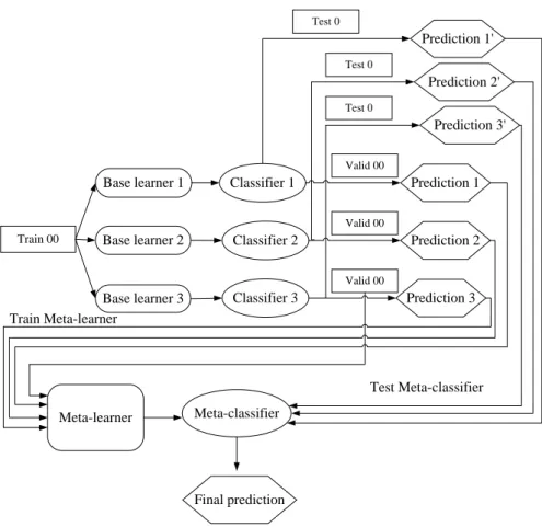
D1 D2 D3 D4 Dn S*n S*1 S*2 S*3 S*42.1.7 Meta-learning Algorithm
According to the earlier sections, meta-learning is a method which encourages diversity implicitly. It also combines the base learners‘ continuous outputs using class-conscious strategies with trainable combiners. Meta-learning can be used to coalesce the results of multiple learners to improve accuracy. It can also be used to combine results from a set of parallel or distributed learning processes to improve learning speed. The methodology that we propose in chapter 3 will concentrate on the first case and the methodology in chapter 4 utilizes the second advantage of meta-learning.
The phenomenon of inductive bias [66] indicates that the outcome of running an algorithm is biased in a certain direction. In the No Free Lunch (NFL) theorems [91], it was stated that there is no universally best algorithm for a broad problem domain. Therefore, it is beneficial to build a framework to integrate different learning algorithms to be used in diverse situations. Here we present the structure of meta-learning.
Meta-learning is usually referred to as a two level learning process. The classifiers in the first level are called base classifiers and the classifier in the second level is the meta-learner. This meta-learner is a machine learning algorithm which learns the relationships between the predictions of the base classifiers and the true class. One advantage of this schema is that adding or deleting the base classifiers can be performed relatively easily since no communications are required between these base classifiers in the first level.
Three meta-learning strategies: combiner, arbiter and hybrid are proposed in [49] to combine the predictions generated by the first level base learners. Here we are focused on the combiner strategy since the methodology we will present in chapter 3 applies this strategy. Depending on how to generate the meta-level training data, there are three schemes as follows:
A.Class-attribute-combiner
In this case a meta-level training instance is composed by the training features, the predictions by each of the base classifiers and true class. In the case of three base classifiers, we represent the predictions of these classifiers on a training instance 𝑋 is {𝑃1(𝑋), 𝑃2(𝑋), 𝑃3(𝑋)}, the attribute vector for 𝑋 is < 𝑥1, 𝑥2, … , 𝑥𝑛 > if the number of attributes is 𝑛, the true class for 𝑋 is 𝑙𝑎𝑏𝑙𝑒(𝑋). Then the meta-level training instance for 𝑋 is
𝑀𝑡 = 𝑃1 𝑋 , 𝑃2 𝑋 , 𝑃3 𝑋 , 𝑥1, 𝑥2, … , 𝑥𝑛, 𝑙𝑎𝑏𝑒𝑙(𝑋) (2.12)
B.Binary-class-combiner
For this rule, the meta-level training instance is made up by all the base classifiers‘ predictions for all the classes and the true class for instance X. The elements in this meta-level training instance basically include all the terms we have shown in equation 2.7 except that the predictions are not probabilities but binary. For example, if we have m numbers of classes and three base classifiers, then the meta-level training instance for X can be expressed as
𝑀𝑡 = 𝑃11 𝑋 , … 𝑃1𝑚 𝑋 , 𝑃21 𝑋 , … 𝑃2𝑚 𝑋 , 𝑃31 𝑋 , … 𝑃3𝑚 𝑋 , 𝑙𝑎𝑏𝑒𝑙(𝑋) (2.13) Here, each prediction for each class is generated by the base classifier which is trained on
the instances which are labeled as the corresponding class or not.
C.Class-combiner
Similar with the Binary-class-combiner, the class-combiner rule also includes the predictions by all the base classifiers and the true class. The difference is that this rule only contains the predicted class from all base classifiers and the correct class. In this case, we express the meta-level training instance as
𝑀𝑡 = 𝑃1 𝑋 , 𝑃2 𝑋 , 𝑃3 𝑋 , 𝑙𝑎𝑏𝑒𝑙(𝑋) (2.14)
In the methodology we will propose in chapter 3, the third rule: class-combiner rule is applied. This combiner rule is not only employed in the training process but also in the testing process to generate the meta-level test data based on the new test instance. The procedure for meta-learning applying the combiner rule is described as follows: for a dataset 𝑆 = { 𝑦𝑛, 𝑥𝑛 , 𝑛 = 1, … , 𝑁} with 𝑦𝑛 as the 𝑛th class and 𝑥𝑛 as the 𝑛th feature
values for instance 𝑛. Then for 𝐽-fold cross validation, this dataset is randomly split into
𝐽 data subsets: 𝑆1, … , 𝑆𝑗, … 𝑆𝐽. For the 𝑗th fold, the test dataset is denoted as 𝑆𝑗 and the training dataset is expressed as 𝑆−𝑗 = 𝑆 − 𝑆𝑗. Then each of the training datasets is again
split randomly into two almost equal folds. For instance, 𝑆−𝑗 is split into 𝑇𝑗1, 𝑇𝑗2. We
assume that there are 𝐿 level-0 base learners.
Therefore, for the 𝑗th round of cross validation, in the training process, first 𝑇𝑗1 is
used to train each the base learners to generate 𝐿 models: 𝑀𝑗11, … , 𝑀𝑗1𝑙, … 𝑀𝑗1𝐿. Then,
𝑇𝑗2 is applied to test each of the generated models to generate the predictions. These predictions are used to form the first part of meta-level training data. The second part of these data is produced by generating the base models on 𝑇𝑗2 and testing the models on
𝑇𝑗1. If there are 𝐺 instances in 𝑆−𝑗 and the prediction generated by model 𝑀𝑗1𝐿 is
denoted as 𝑍𝐿𝑔 for instance 𝑥𝑔, then the generated meta-level training data can be
expressed as
𝑆𝐶𝑉 = 𝑍1𝑔, … , 𝑍𝐿𝑔,𝑦𝑔 , 𝑔 = 1, … , 𝐺 (2.15) This meta-level training data is the combination of the first and second parts‘ predictions. Based on these data, the level-1 model is generated as 𝑀. The last step in the training process is to train all the base learners on 𝑆−𝑗 to generate the final level-0 models:
𝑀1, … 𝑀𝑙, … 𝑀𝐿. The whole training process is also shown in fig.2.6.
M
~
) ( S j Level_1 Level_0 1 jT
T
j2 11 jM
...
M
j1l...
Mj1LM
j21...
M
j2l...
M
j2L cvS
Fig.2.6. Meta-learning training process for fold 𝑗
In the test process, to generate the meta-level test data, 𝑆𝑗 is used to test the level-0 base models 𝑀1, … 𝑀𝑙, … 𝑀𝐿generated in the training process. For instance, for the instance 𝑥𝑡𝑒𝑠𝑡in 𝑆𝑗, the meta-level test instance can be obtained as (𝑍1, … , 𝑍𝑙, … , 𝑍𝐿 ). All the meta-level test data are feed into the meta-level model 𝑀 to generate the predictions for these test data. We also present the pseudo code for the meta-learning training algorithm for the 𝑗th cross validation training process in table 2.2.
Table 2.2. Meta-learning algorithm for training process
Input:
Training dataset: 𝑆−𝑗
Meta learning algorithms:𝐶𝑚
Base learning algorithms: C1, C2, … , CL
Output: Ensemble 𝐸 1. 𝐸 = ∅ 2. 𝑆𝑐𝑣 = ∅ 3. 𝑇𝑗1, 𝑇𝑗2 = SplitData(𝑆−𝑗, 2) 4. For𝑙 = 1 to 𝐿do 5. 𝑀𝑗1𝑙 = 𝐶𝑙 𝑇𝑗1 6. 𝑀𝑗2𝑙 = 𝐶𝑙 𝑇𝑗2 7. End for 8. 𝑆𝑐𝑣1 = 𝑀𝑗11 𝑥𝑖 , 𝑀𝑗12 𝑥𝑖 , … 𝑀𝑗1𝐿 𝑥𝑖 , 𝑦𝑖 9. 𝑆𝑐𝑣2 = 𝑀𝑗21 𝑥𝑘 , 𝑀𝑗22 𝑥𝑘 , … 𝑀𝑗2𝐿 𝑥𝑘 , 𝑦𝑘 10. 𝑆𝑐𝑣 = 2𝑖=1𝑆𝑐𝑣𝑖 11.𝑀 = 𝐶𝑚 𝑆𝑐𝑣 12. 𝑀1, 𝑀2, … 𝑀𝐿 = 𝐶1 𝑆−𝑗 , 𝐶2 𝑆−𝑗 , … , 𝐶𝐿(𝑆−𝑗) 13. 𝐸 = 𝑀1, 𝑀2, … 𝑀𝐿 , 𝑀 14.Return 𝐸
2.2 Large Scale Machine Learning
Although the MapReduce framework is very popular in the industry for cloud computing, its power to construct scalable machine learning algorithms is rarely recognized in the academic field. Basically, to construct scalable machine learning algorithms using MapReduce, knowledge of the following three components are indispensible: the Hadoop platform which is an open source implementation of MapReduce, the MapReduce programming framework and the Hadoop distributed file system. Being acquainted with their roles in the system is beneficial for us to construct new scalable machine learning algorithms. In addition to MapReduce and Hadoop some other low-level and high-level systems were also proposed in the very recent years. The active research in the scalable machine learning area is boosting its development to a new level in the future.
This section first discusses the datasets which can be categorized as large scale for machine learning algorithms and then proceeds to introduce Hadoop, MapReduce and Hadoop distributed file systems which are the three pillars for implementing scalable machine learning algorithms with MapReduce. Finally, some recent advances in methodologies and systems for scalable machine learning are presented and the motivation for our proposal of the methodology in chapter 4 is also presented.
2.2.1 Large Scale Datasets
Here we discuss the spectrum of ‗large scale‘ not according to their respective domains but to the characteristics of the problem. The most relevant method to determine ‗large scale‘ is through the number of records. For example, the genetic sequences database of the US National Institute of Health: GenBank3 contains more than 125
million gene sequences and more than 118 billion nucleotides on October 2010 while the corresponding numbers are 82 million and 85 billion in 2008. Up to 700 megabytes of data can be generated per second by the Large Hadron Collider4. Moreover, up to 1
billion base pairs can be sequenced by the next-generation sequencing technologies in a single day [67]. Furthermore, the large records of data not only come from the natural sciences but also from the industry. For instance, one of the most famous data mining challenges in the latest years: Netflix prize5 released an anonymized version of their
movie ratings database of over 100 million ratings from 480,000 customers and 18,000 movies. The public was challenged to provide a recommendation algorithm which outperforms by 10% their own proprietary method.
Another challenging aspect is the number of variables of the problem. As an example, one of the most widespread technologies of molecular biology research: microarray analysis [68] usually generates data having few records with tens of thousands
3Genbank release notes. Available at: ftp://ftp.ncbi.nih.gov/genbank/gbrel.txt.
4 Physicists brace themselves for LHC ‗data avalanche‘. Available at:
of variables as the generation of each record is very expensive. As a result, there is a very high imbalance between records and variables and many machine learning algorithms tend to overfit this kind of data. Another example in the natural sciences domain is protein structure prediction (PSP)6 which also generates datasets which have far more
number of variables than records.
Last but not least, the large number of classes is also another source of difficulty for machine learning methods. The most well-known example happens in the information retrieval/text mining area where datasets have an extremely high number of classes7. The
other two class related difficulties are for datasets which have a hierarchical structure of the class and certain classes have very low frequency (the class imbalance problem [69]). Although this class imbalance problem cannot be considered as a difficulty specially for large scale data mining as it also happens for small data sets, it could become a recurrent problem when datasets grow and tend to become more heterogeneous.
In sum, the question we are trying to answer is when a dataset becomes large scale. This is not an easy question to address as it depends on the type of learning tasks and resources available to analyze the data. The simplest answer is when a dataset‘s size starts to become an issue to take into account explicitly in the data mining process8. If an
algorithm only needs to process the training set through one single pass, it would be easy for the algorithm to process hundreds of millions of records. However, in reality an algorithm usually needs to use the training set over and over again. In this case, the
6 The ICOS PSP benchmarks repository. Available at: http://icos.cs.nott.ac.uk/datasets/psp_benchmark.html.
7Reuters-21578 text categorization collection. Available at: http://kdd.ics.uci.edu/databases/reuters21578/reuters21578.html. 8Dumbill E. What is big data?, 2012. Available at: http://radar.oreilly.com/2012/01/what-is-big-data.html
algorithm struggles with only a few tens of thousands of instances. The same thing happens with the number of attributes (variables).
2.2.2 Hadoop
Large scale data has brought both benefits and challenges. One of the benefits is that we can extract lots of useful information by analyzing such big data. Extracting knowledge from massive data sets has attracted tremendous interest in the data mining community. In the field of natural language processing, it was concluded [70] that more data leads to better accuracy. That means, no matter how sophisticated the algorithm is, a relatively simple algorithm will beat the complicated algorithm with more data. One practical example is recommending movies or music based on past preferences [71].
One of the challenges is that the problem of storing and analyzing massive data is becoming more and more obvious. Although the storage capacities of hard drives have increased greatly over the years, the speeds of reading and writing data have not kept up the pace. Reading all the data from a single drive takes a long time and writing is even slower. Reading from multiple disks at once may reduce the total time needed, but this solution causes two problems.
The first one is hardware failure. Once many pieces of hardware are used, the probability that one of them will fail is fairly high. To overcome this disadvantage, redundant copies of the data are kept, in case of data loss. This is how Hadoop‘s file system: Hadoop Distributed File System (HDFS) works. The second problem is how to
combine data from different disks. Although various distributed systems have provided ways to combine data from multiples sources, it is very challenging to combine them correctly. The MapReduce framework provides a programming model that transforms the disk reads and writes into computations over sets of keys and values.
Hadoop is an open source Java implementation of Google‘s MapReduce algorithm along with an infrastructure to support distribution over multiple machines. This includes its own filesystem HDFS (based on the Google File System) which is specifically tailored for dealing with large files. MapReduce was first invented by engineers at Google as an abstraction to tackle the challenges brought about by large input data [8]. There are many algorithms that can be expressed in MapReduce: from image analysis, to graph-based problems, to machine learning algorithms.
In sum, Hadoop provides a reliable shared storage and analysis systems. The storage is provided by HDFS and the analysis by MapReduce. Although there are other parts of Hadoop, these two are its kernel components.
2.2.3 MapReduce
MapReduce simplifies many of the difficulties in parallelizing data management operations across a cluster of individual machines and it becomes a simple model for distributed computing. Applying MapReduce, many complexities, such as data partition, tasks scheduling across many machines, machine failures handling, and inter-machine communications are reduced.
Promoted by these properties, many technology companies apply MapReduce frameworks on their compute clusters to analyze and manage data. In some sense, MapReduce has become an industry standard, and the software Hadoop as an open source implementation of MapReduce can be run on Amazon EC29
. At the same time, the
company Cloudera10
offers software and services to simplify Hadoop deployment. Several universities have been granted access to Hadoop clusters by Google, IBM and Yahoo! to advance cluster computing research.
However, MapReduce‘s application to the machine learning tasks is poorly recognized despite of its growing popularity. It is natural to ask the question whether the MapReduce-capable compute infrastructure could be useful in the development of parallelized data mining tasks with the wide and growing availabilities of such infrastructures.
A.MapReduce Framework
As a programming model to process big data, there are two phases included in the MapReduce programs: Map phase and Reduce phase [72]. The programmers are required to program their computations into Map and Reduce functions. Each of these functions has key-value pairs at their inputs and outputs. The input is application-specific while the output is a set of <key, value> pairs, which are produced by the Map function. The key and value pairs are expressed as follows:
𝑘1, 𝑣1 , … , 𝑘𝑛, 𝑣𝑛 : ∀𝑖 = 1 … 𝑛 ∶ (𝑘𝑖 ∈ 𝐾, 𝑣𝑖 ∈ 𝑉) (2.16)
Here 𝑘𝑖represents key for the 𝑖𝑡 input and 𝑣𝑖 denotes the value for the 𝑖𝑡 input. 𝐾