Development of a New Tracking System based on CMOS Vision Processor Hardware: Phase I

Development of a New Tracking System based on

CMOS Vision Processor Hardware: Phase I

Final Report

Prepared by: Hua Tang

Department of Electrical and Computer Engineering University of Minnesota Duluth

Northland Advanced Transportation Systems Research Laboratory University of Minnesota Duluth

Technical Report Documentation Page

1. Report No. 2. 3. Recipients Accession No.

CTS 09-04

4. Title and Subtitle 5. Report Date

February 2009

6.

Development of a New Tracking System based on CMOS

Vision Processor Hardware: Phase I

7. Author(s) 8. Performing Organization Report No.

Hua Tang

9. Performing Organization Name and Address 10. Project/Task/Work Unit No.

CTS Project # 2008016

11. Contract (C) or Grant (G) No.

Department of Electrical and Computer Engineering University of Minnesota Duluth

1023 University Dr

Duluth, Minnesota 55812

12. Sponsoring Organization Name and Address 13. Type of Report and Period Covered

Final Report

14. Sponsoring Agency Code

Intelligent Transportation Systems Institute Center for Transportation Studies

University of Minnesota

511 Washington Avenue SE, Suite 200 Minneapolis, Minnesota 55455

15. Supplementary Notes

http://www.cts.umn.edu/Publications/ResearchReports/

16. Abstract (Limit: 200 words)

It is well known that vehicle tracking processes are very computationally intensive. Traditionally, vehicle tracking algorithms have been implemented using software approaches. The software approaches have a large computational delay, which causes low frame rate vehicle tracking. However, real-time vehicle tracking is highly desirable to improve not only tracking accuracy but also response time, in some ITS (Intelligent Transportation System) applications such as security monitoring and hazard warning. For this purpose, this project proposes a hardware based vehicle tracking system for real-time high frame rate tracking. The proposed tracking algorithm is based on motion estimation by full-search block matching algorithm. Motion estimation is implemented in a hardware processor, which could significantly reduce the computational delay compared to traditional software approaches. In this project, the hardware processor is first designed and verified using Cadence software in CMOS (Complementary Metal Oxide Semiconductor) IBM 0.13μm technology, and then mapped to the Xilinx Spartan-3A DSP Development Board for quick implementation. Test results have shown the hardware processor functions correctly with sequences of traffic images. We also design the algorithms to post-process the motion vectors output from the hardware processor to complete the overall vehicle tracking process.

17. Document Analysis/Descriptors 18. Availability Statement

Vehicle tracking, video-based tracking, image sensor, real-time operation, hardware implementation

No restrictions. Document available from: National Technical Information Services, Springfield, Virginia 22161

19. Security Class (this report) 20. Security Class (this page) 21. No. of Pages 22. Price

Development of a New Tracking System based on

CMOS Vision Processor Hardware: Phase I

Final Report

Prepared by Hua Tang

Department of Electrical and Computer Engineering University of Minnesota Duluth

Northland Advanced Transportation Systems Research Laboratory University of Minnesota Duluth

February 2009

Published by

Intelligent Transportation Systems Institute Center for Transportation Studies

University of Minnesota

511 Washington Avenue SE, Suite 200 Minneapolis, Minnesota 55455

The contents of this report reflect the views of the authors, who are responsible for the facts and the accuracy of the information presented herein. This document is disseminated under the sponsorship of the Department of Transportation University Transportation Centers Program, in the interest of

information exchange. The U.S. Government assumes no liability for the contents or use thereof. This report does not necessarily reflect the official views or policy of the Intelligent Transportation Systems Institute or the University of Minnesota.

The authors, the Intelligent Transportation Systems Institute, the University of Minnesota and the U.S. Government do not endorse products or manufacturers. Trade or manufacturers’ names appear herein solely because they are considered essential to this report.

Acknowledgments

I would like to thank Dr. Eil Kwon, director of Northland Advanced Transportation Systems Research Laboratory (NATSRL), and Dr. Taek Kwon, professor in the Electrical and Computer Engineering Department at University of Minnesota Duluth, for their valuable discussions and comments. Also, I would like to acknowledge the great efforts in implementing the proposed vehicle tracking system by my graduate students, Yi Zheng and Peng Li.

I would like to acknowledge those who made this research possible. The study was funded by the Intelligent Transportation Systems (ITS) Institute, a program of the University of Minnesota’s Center for Transportation Studies (CTS). Financial support was provided by the United States Department of Transportation’s Research and Innovative Technologies Administration (RITA). The project was also supported by NATSRL, a cooperative research program of the Minnesota Department of Transportation, the ITS Institute, and the University of Minnesota Duluth College of Science and Engineering.

Table of Contents

Chapter 2 Overview of the Proposed Vehicle Tracking System ... 5

2.1 Introduction... 5

2.2 Overall Processing Flow ... 5

2.3 Step 1: Image Read In... 6

2.4 Step 2: Motion Estimation Based On Block Matching... 6

2.4.1 Illustration of Step 2 for Vehicle Tracking ... 7

2.5 Step 3: Transmission of Motion Vectors to PC ... 8

2.6 Step 4: Vehicle Tracking In Software... 8

2.7 Comparison with Conventional Tracking Algorithm ... 10

2.8 Summary ... 12

Chapter 3 Hardware Design of Motion Estimation Algorithm... 13

3.1 Introduction... 13

3.2 Timing Budget ... 13

3.2.1 Time of Frame Transmitting... 14

3.2.2 Time of Block Matching... 14

3.3 Design Details of Hardware Processor ... 15

3.3.1 Memory Design ... 15

3.3.2 Block Matching Algorithm Implementation... 16

3.3.3 Design of Control Signal Generator ... 21

3.3.4 Design of System Clock Signal Generator ... 23

3.3.5 Entire Hardware Part... 24

3.4 Interface Unit ... 25

3.5 Logic Simulation Result ... 25

Chapter 4 Design of Software Part of the Tracking System... 27

4.1 Introduction... 27

4.2 Blob Extraction ... 27

4.2.1 Noise Removal... 28

4.2.2 Blob Segment Detection ... 29

4.2.3 Complete Blob Detection... 30

4.3 Blob Association... 32

4.3.1 One-to-many Association ... 34

4.3.2 Many-to-one Association... 34

4.3.3 No Association... 35

4.4 The Entire Software Implementation... 35

4.5 Summary ... 36

Chapter 5 Test of the Vehicle Tracking Algorithm ... 38

5.1 Introduction... 38

5.2 Tracking of Two Vehicles ... 38

5.3 Tracking of Four Vehicles ... 39

5.4 Tracking of Vehicle Turning ... 40

5.5 Limitations ... 43 5.6 Summary ... 46 Chapter 6 Conclusion... 47 6.1 Summary ... 47 6.2 Conclusions... 47 6.3 Future Work ... 47 References... 48

List of Figures

Figure 2-1: Overall system diagram of the proposed tracking system ... 6

Figure 2-2: Motion estimation based on full search block matching... 7

Figure 2-3: A traffic image captured at an intersection (frame N-1) ... 9

Figure 2-4: A traffic image captured at an intersection (frame N) ... 9

Figure 2-5: Block motion of frame (N-1) with respect to frame (N)... 10

Figure 2-6: An illustration of conventional tracking algorithms ... 11

Figure 3-1: The hardware processor for motion estimation... 13

Figure 3-2: Commercial Micron image sensor system ... 15

Figure 3-3: Synchronous Single-Port SRAM Diagram ... 16

Figure 3-4: The hardware architecture to implement FBMA ... 17

Figure 3-5: The architecture of systolic array... 18

Figure 3-6: Block diagram of PEi, j... 19

Figure 3-7: Block diagram of the shift register array (SRAi) ... 19

Figure 3-8: Block diagram of the best match-selection unit... 20

Figure 3-9: Block diagram of the control unit ... 21

Figure 3-10: The regions of valid and invalid MAD values... 21

Figure 3-11: Block diagram of the control signal generator... 22

Figure 3-12: The original and new buffer control signals ... 24

Figure 3-13: Alternative SRAM switching to store new frame data ... 24

Figure 3-14: The diagram of entire hardware part... 24

Figure 3-15: Pesudo-code for reading data from the buffer ... 25

Figure 3-16: Logic simulation result... 25

Figure 4-1: An overview of the proposed tracking algorithm ... 27

Figure 4-2: An illustration of noise removal... 28

Figure 4-3: Pseudo-code for noise removal ... 29

Figure 4-4: Pseudo-code for blob segment detection ... 30

Figure 4-5: A Matrix storing the size of blob segments ... 30

Figure 4-6: A matrix storing motion status of blob segments ... 30

Figure 4-7: Pseudo-code for extracting the blob from BMRF... 31

Figure 4-9: Extracted blob from BMRF (N)... 32

Figure 4-10: An illustration of the proposed tracking algorithm... 33

Figure 4-11: Pseudo-code for blob association... 34

Figure 4-12: Pseudo code of the entire software component... 36

Figure 4-13: An illustration of the result of blob association ... 37

Figure 5-1: System timing ... 38

Figure 5-2: The image frame (20) and (40) for the first test... 39

Figure 5-3: The tracked trajectories of the vehicles for the first test ... 39

Figure 5-4: The image frame (20) and (80) for the second test ... 40

Figure 5-5: The tracked trajectories of the vehicles for the second test ... 40

Figure 5-6: The image frame (1) and (30) for the third test... 41

Figure 5-7: An illustration of the possible issue for vehicle turning ... 42

Figure 5-8: An illustration of how to solve the issue... 42

Figure 5-9: The tracked trajectories of the vehicles for the third test ... 43

Figure 5-10: Three consecutive image frames of a ring intersection... 44-45 Figure 5-11: Two resulting BMRFs... 45

Executive Summary

It is well known that vehicle tracking processes are computationally very intensive. In the past, regardless of different algorithms employed in vehicle tracking, they have been implemented using software approaches. While software approaches have an advantage of flexibility in implementation and future modifications, their long computational time often prevents real-time vehicle tracking from high resolution spatial or temporal data. This gives rise to a need for direct implementation of tracking algorithms in hardware.

The goal of the proposed project is to build a hardware-based vehicle tracking system to improve real-time high frame rate vehicle tracking, which would help improve tracking accuracy as well as response time. The overall project is divided into two phases. In phase I, which is this report describes, we plan the overall tracking algorithm for the hardware-based vehicle tracking systems, design each of the building components in the system, and finally, actually implement it. Following phase I, we will be synthesize the overall vehicle tracking system, build a system prototype and actually test it in the field.

Designing a hardware-based vehicle tracking system involves not only hardware implementation, but also the overall tracking algorithm that is well suited to hardware implementation. Therefore, the two main tasks in this project are to first design the overall tracking algorithm and then implement it in hardware.

For the first task, we propose a new tracking algorithm based on vehicle motion estimation, which is implemented in hardware whenever possible so that the computation time for tracking is minimized. The motion detection is based on the popular block-matching algorithm used in image processing applications. The main idea of motion estimation is to divide each image frame into a number of smaller-size blocks and match two consecutive image frames to output motion vectors, which identify where and how each block of the image frame moves between the two consecutive image frames. Depending on the block size and vehicle size in the image frame, an object or a vehicle may consist of one or more image blocks. Given motion vectors, the image blocks that have the same or very similar motion vectors are grouped as one or more vehicles. This step of processing is called vehicle extraction. One or more vehicles can be extracted between any two consecutive image frames using motion estimation, and the other step of processing called vehicle association is used to relate vehicles extracted from two consecutive motion estimations, which actually spans three consecutive image frames. Therefore, the vehicles can be tracked by tracking what image blocks constitute the vehicles and how they move with the help of the motion vectors.

The processing flow of the overall tracking system is then as follows:

• Step 1: an image sensor captures images at a high frame rate, for example, 30-60 frames/sec. Note that this assumption has to be validated by relatively short computational time for our approach.

• Step 2: each captured image frame is subject to Gaussian noise filtering to remove the thermal noise.

• Step 3: two consecutive image frames are block-wise matched to output motion vectors for each image block.

• Step 4: the motion vectors are analyzed to identify moving vehicles and track how and where each vehicle moves.

To verify the tracking algorithm, we implement the tracking system in MATLAB computing software in a PC. Feeding realistic traffic images, the tracking system is shown to be able to track vehicles in most cases.

After defining and verifying the overall vehicle tracking algorithm, we implement the overall tracking system in hardware to allow real-time vehicle tracking. Therefore, the other main task of the project is to implement a CMOS hardware processor for vehicle motion detection. As a short processing time is desired, the systolic array processing architecture is adopted to allow parallel block matching computation. The hardware processor is first designed in Cadence using IBM 0.13μm technology and verified by behavioral-level simulators. Then the hardware processor is mapped to Xilinx Spartar-3A DSP development board for actual implementation. Feeding the same traffic images, the results show that the developed hardware functions correctly. In addition, the hardware processor completes one block matching for two consecutive images within 6 milli-seconds, which may pave the way for high frame rate vehicle tracking if the rest of the processing steps do not take significant time.

The proposed vehicle tracking system and its hardware implementation have quite a few advantages compared to traditional systems and implementations. First, the system is more adaptable to different whether conditions, as the tracking algorithm is based on relative vehicle shift without the use of a static background image. Second, hardware implementation of the proposed tracking system achieves high frame rate tracking, thus improves real-time response and tracking accuracy. In phase II of the project, we will synthesize the hardware processor with other components to build a prototype of the tracking system, and then test it in the field.

In spite of the above potential advantages of the proposed tracking system, future work needs to be done to fully take advantage of the system. For example, it is found that motion estimation may be vulnerable to camera jittering effect, which prevents the correct motion vectors output. Also, vehicle tracking based on the information provided solely by the motion vectors may limit the use of the system in highly congested and highly occluded traffic areas.

Chapter 1

Introduction

1.1 Introduction

Vehicle tracking is an important area of Intelligent Transportation Systems (ITS), which could be applied in a wide range of transportation applications. In vehicle tracking, the general purpose is to accurately track the vehicle moving trajectory. General purpose vehicle tracking has many applications, such as vehicle detection, intersection monitoring, vehicle counting etc [1]. If high frame rate vehicle tracking is available, it can be applied in security monitoring and hazard warning applications. For example, a collision warning can be issued when two vehicles are too close to each other [2]. Vehicle tracking systems have been previously developed using different methods, like microwave radar, video, or a combination of both [3].

In our project, the video-based vehicle tracking method is used. The video-based vehicle tracking approach has quite many advantages, such as convenience of installation, low cost operation, possible large coverage of the area of interests, and non-intrusiveness. Today, many video-based vehicle tracking systems are available, such as those reported in [4][5][6], even some commercial systems, such as the AutoScope tracking systems from Image Sensing Systems Inc. [7].

Vehicle tracking typically needs to monitor real-time vehicle movements, and thus real time operation is highly desirable. However it is well known that vehicle tracking processes are very computationally intensive. In the past, regardless of different algorithms employed in vehicle tracking, they have been implemented using software approaches, e.g., FPGA (Field Programmable Gate Array), micro-controllers, microprocessors, or Personal Computers (PC). While software approaches have an advantage of flexibility in implementation and future modifications, its long computational time often prevents real-time vehicle tracking from spatial or temporal high resolution data. It is well known in the area of VLSI (Very Large Scale Integrated) circuit design that a dedicated hardware implementation of any algorithm minimizes its computational time [8]. This is the motivation for direct implementation of tracking algorithms in hardware (i.e., device level), whether it is a partial or full implementation.

1.2 Previous Work

In this section, we briefly review some previous vehicle tracking systems and their implementations. For example, reference [4] presents a method for tracking and counting pedestrians or vehicles using a single camera. In order to accurately capture important movement information, the system must acquire pictures at a high-frame rate. However, due to a large computational delay required by software implementation of the tracking algorithm, a high frame rate or a high resolution is difficult to achieve.

The tracking algorithm in [4] is divided into three phases of operations: raw image processing, blobs graph optimization and Kalman filtering based estimation of object parameters. First, at the raw image level, Gaussian noise filtering, background subtraction and thresholding is

performed to produce binary difference images in 256×256 pixels. The difference images are then supplied to the next phase of operation, where the changes with respect to two consecutive difference images are described in terms of motions of blobs. After extracting blobs from the difference images, blob motions with respect to two consecutive difference images is modeled as a graph optimization problem for which the overall goal is to find the blob motions that cause the smallest amount of size change with respect to two consecutive difference images. Note that in this process, additional constraints are enforced in order to make the graph manipulation computationally tractable [4]. But these constraints are based on the assumption that images are captured in a very high frame rate (which may contradict the actual situation of being not high frame rate). Blob graph optimization requires a lot of computational resources due to its iterative and enumerative processes. In the final phase of the tracking algorithm, Extended Kalman Filtering (EKF) is used to estimate object parameters. Note that, the computational requirement of Kalman filtering is quite high [4][9]. Without a proper timing control of Kalman filtering, the overall tracking performance may degrade significantly [4][9].

The overall tracking algorithm in [4] is implemented on a Datacube MaxVideo 20 video processor and a Max860 vector processor and is later ported to use 400MHz Pentium PC with C80 Matrox Genesis vision board. For the software implementation of tracking algorithm, peak frame rate is reported to be 30 frames per second while in many cases it drops to a few frames per second depending on the number of objects and weather conditions, which may present significant problems in tracking accuracy [4]. An inherent conflict exists between the requirement of higher time and space resolution (or to have high frame rate) and the requirement of a longer computational time by the software implementation. Note that the same tracking algorithm presented in [4] has been applied to many other cases, such as [5] [6] and the same software approach is used.

Software implementation of tracking algorithm experiences a severe time-crunch problem when the algorithm is to improve the tracking performance by adding more processing steps. For example, considering the shape of objects being tracked adds a considerable amount of computational overhead [4]. Detection and classification of vehicles can only be done for two general classes (cars versus trucks), because further classifying the vehicles for the two classes significantly lengthens the computational time and prevents real-time classifications of vehicles [6]. To improve the tracking accuracy, some other operations, such as shadow removing, is required, which again takes significant amount of computational time [10]. As a result, implementation approaches that are software dominant may not meet the computationally demanding requirement of real-time operations.

1.3 Motivation

The speed limitation of software approaches for vehicle tracking system implementation motivates us to look for alternative methods. For vehicle tracking, there are two ways to improve real-time operations. One is to develop a new tracking algorithm that is simpler and faster, thus requiring less computational time. While this is feasible and has been under research [4], a tradeoff exists between the tacking accuracy and algorithm complexity. In general, the more complex the tracking algorithm is, the more accurate the tracking is, so the longer the computational time is.

A more plausible solution to reduce computational delay of tacking algorithm is to implement the algorithm in hardware [8]. Motivated by the limitations of the software approaches for vehicle tracking, there have been recent research interests in hardware implementation of algorithms used in different areas of ITS applications. Yang proposes a 256×256-pixle Complementary Metal Oxide Semiconductor (CMOS) image sensor used in line-based vision applications [11]. Nakamura implements a sensor with inherent signal processing functionalities [12]. Fish also implements a CMOS filter which can be used in lane detection applications [13]. Hsiao uses circuit design techniques from previous works [11][12][13] and proposes a hardware implementation of a mixed-signal CMOS processor with built-in image sensor for efficient lane detection for use in intelligent vehicles [14]. Hsiao does not compare the computational time of the processor to that of software implementation for the lane detection algorithm, but it is shown that a hardware approach can even improve the performance of simple lane detection [14].

Drawing from current and future demands for real-time operations of vehicle tracking, this project intends to develop a new tracking system largely based on hardware implementation. Note that the main initiative to implement a CMOS vision processor is to improve real-time operation of vehicle tracking, since a hardware implementation of the tracking algorithm could significantly improve the processing speed compared to the software approach. In addition, a few other advantages can be identified for hardware implementation of tracking algorithm. First, the performance of real-time vehicle tracking will be improved. Many other tasks that previously could not be incorporated in the tracking process due to computational time constraint may now be enabled. Second, potential improvements on tracking accuracy are expected due to high-frame rate tracking. For instance, the performance of lane detection for a CMOS processor is improved compared to that of the software approach, as reported in [14]. In fact, from the VLSI circuit design point of view, a dedicated hardware has less undesired effects, such as accumulated digitization error [8]. Another benefit is that the hardware size could be much smaller compared to micro-controllers (software implementation), thus the overall system will be more portable. Moreover, the power consumption of dedicated hardware will potentially be much less compared to software implementations [8]. This feature would be especially important in the future effort to design low-power tracking systems. Even more importantly, the cost of the tracking system could be reduced to a fraction of that of software implementations. But some potential disadvantages of the hardware approach are also identified. First, the initial development cost may be huge, and the design cycle for a hardware processor is typically much longer than that of the software approach. This possible huge design effort could be only compensated for by extensive usage of the developed hardware in real ITS applications. Second, typically a hardware approach is not as flexible as a software approach. In the software approach, designers only need to change the software codes to adapt to new situations, whereas the hardware approach may not be easily adapted to new situations. Though reconfigurable design techniques can be applied during the hardware design to achieve flexibility, this is at the expense of extra design effort and hardware components [8].

The main initiative of hardware implementation of tracking algorithm is to minimize the computational time and thus to improve real-time operation of vehicle tracking, but directly proceeding to hardware implementation of a tracking algorithm may make the overall design process impractical considering other factors. The other factors that have to be considered for hardware design include the overall development cost, the overall hardware complexity (design

cycle) and the required flexibility [8] as mentioned above. If the overall development cost is prohibitively high, then a software approach to implement tracking algorithm should be favored since micro-controllers are much cheaper. Similarly, if the design cycle is too long (time-to-market is thus seriously delayed), hardware implementation is also at a disadvantage. Considering all these factors, a strong argument for hardware implementation is that the hardware can be designed in a way that is both time and cost effective, and the hardware will be designed to be re-useable in different tracking algorithms [8]. The later also relates well to the area of Hardware/Software Co-design [8] since some processing steps of the tracking algorithm are more suited to hardware implementation while the others are to software implementation. Considering all these factors, simply taking an existing tracking algorithm, such as the one in [4][5][6], and implementing it in hardware may not result in a good solution. In fact, analysis shows that implementing the tracking algorithm in pure hardware [4][5][6] is very costly. But on the other hand, if only some parts of the tracking algorithm are implemented in hardware, the overall computational time saving is not promising. As a result, improving real-time operation of tracking is more than just pure hardware implementation, but instead it requires also innovation in both tracking algorithm design, which has to be well suited to hardware design with reasonable design effort.

In this project, we propose a possible solution to design a hardware-based vehicle tracking system and its hardware implementations.

1.4 Summary

In this chapter a brief review of the traditional vehicle tracking system is provided. The advantages and disadvantages of the conventional tracking systems based on software implementation are discussed. Possible hardware implementation of vehicle tracking system is also proposed in order to improve frame rate and the real time operation of the vehicle tracking. The organization of the rest of the report is described as follows:

• In Chapter 2, an overview of the proposed vehicle tracking system is provided and its core tracking algorithm based on motion estimation is presented in detail;

• Chapter 3 details on how to implement motion estimation algorithm in hardware and how to interface the hardware to image sensor and the PC;

• Chapter 4 describes the design of the post-processing software for processing the motion vector outputs from the hardware processor;

• In Chapter 5, some simulation and test results of the tracking system for validating the vehicle tracking algorithm are provided;

Chapter 2

Overview of the Proposed Vehicle Tracking System

2.1 Introduction

Motivated by the limitation of software implementation for vehicle tracking systems discussed in Chapter 1, this chapter proposes a vehicle tracking system based on hardware implementation and discusses its overall processing flow. The system includes two parts which are implemented by hardware and software separately. The commercial image sensor, Micron MT9V111, is used to capture traffic images, and the data outputs are sequences of image frames [15]. The images frames will be transmitted to the hardware processor, which implements the core of the tracking algorithm, motion estimation based on block matching algorithm. Once the motion vectors are computed, they are transmitted to the software part (a PC computer for current implementation) through a high-speed Universal Serial Bus (USB) interface. Finally, the developed MATLAB code processes the motion vectors to track vehicles. This completes one tracking cycle.

2.2 Overall Processing Flow

The processing flow of the proposed tracking system is explained as follows and the diagram is shown in Figure 2-1:

• Step 1: it is assumed that an image sensor captures images at a high frame rate. However, this high frame rate needs to be validated by relatively short computational time for the proposed approach so that there is no contradiction between assumed high frame rate and actual low processing speed as in conventional tracking system [4][5][6].

• Step 2: two consecutive image frames are first stored and then matched to identify object motion (in this case, the objects are vehicles). The motion detection is based on the full-search block matching algorithm. The outputs of the block matching computation are the motion vectors of all blocks in the image frames.

• Step 3: the motion vectors are transmitted to the next stage of processing by going through the interface unit which is used to connect the designed hardware processor to the computer.

• Step 4: in this final step, blob extraction and blob association are conducted by processing the data transmitted from the previous step to identify moving vehicles and track how and where each vehicle moves.

For the proposed tracking algorithm, step one to step three are well suited to hardware implementation, whereas the final step is currently put to software implementation, but can be mapped to hardware implementation too. As a result, the proposed plan to implement the tracking system is to design a CMOS hardware processor for motion detection and then a software program on a PC for vehicle association and tracking. It is a good tradeoff between computational time and development cost. The hardware processor for motion detection can be widely used in many image processing applications and ITS applications [16]. Therefore,

hardware implementation of the core tracking algorithm is worthy of the possible high development cost and design effort.

Figure 2-1: Overall system diagram of the proposed tracking system 2.3 Step 1: Image Read In

There is no need to build a customized image sensor since it is already commercial available. In the proposed vehicle tracking system a MT9V111 Micron Image Sensor with demo kit [17] is used. The Micron Imaging MT9V111 is a 1/4-inch Video Graphics Array (VGA)-format CMOS active-pixel digital image sensor, with the programmable frame rate up to 60 frames per second (fps), which can meet the real-time requirement of vehicle tracking [15].

2.4 Step 2: Motion Estimation Based On Block Matching

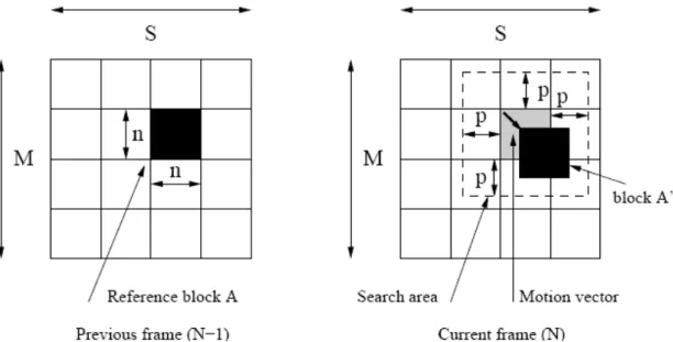
The hardware processor implements the core of the tracking algorithm, motion estimation based on block matching algorithm. An illustration of block matching algorithm is shown in Figure 2-2. Suppose that the image size is M×S (in pixels) and the block size is n×n, then a total of (M×S)/(n×n) blocks are defined for each image frame (for illustration purpose, Figure 2-2 shows only 16 blocks for each frame). With respect to two consecutive images, shown as “current frame” (say frame number N) and “previous frame” (frame number N-1) in Figure 2-2, reference block A (the dark shaded region) in “previous frame” can be considered as a moved version of block A’ in “current frame” and block A’ is in the neighborhood area of the A. This neighborhood, called search area, is defined by parameter, p, in four directions (up, down, right and left) from the position of block A. The value of p is determined by the frame rate and object speed. If the frame rate is high, as assumed in the proposed tracking system, then parameter p can be set relatively small since the block A is not expected to move dramatically within a short period of time. In the search area of (2p+n)×(2p+n), there are a total of (2p+1)×(2p+1) possible candidate blocks for A and the block A’ in “current frame” (N) that gives the minimum matching value is the one that originates from block A in “previous frame” (N-1). The most commonly used matching criterion, MAD (Mean Absolute Difference), is defined as follows [16]:

,|

)

,

(

)

,

(

|

)

,

(

∑

∑

−

+

+

=

j

i

R

v

j

u

i

S

v

u

MAD

−

p

≤

(

u

,

v

)

≤

p

where is the reference block of size n×n, is the candidate block within the search area and represents the block motion vector. The motion vectors computed from block matching contain information on how and where each block in the image moves within two consecutive image frames.

Figure 2-2: Motion estimation based on full search block matching 2.4.1 Illustration of Step 2 for Vehicle Tracking

Due to multiple factors, such as noises, frame rate and block size, the motion vectors computed for the blocks that belong to the same vehicle may be different, which makes the tracking system hard to correctly identify the vehicle and extract it. Therefore, in the proposed tracking system, the motion status is processed instead of the raw motion vectors. To obtain the motion status, the motion vectors are quantized based on the following definitions. Suppose that a block A has original coordinates as (x, y) in “previous frame” (N-1). To be consistent, the origin (0, 0) is defined as the coordinates of the upper-left corner of a rectangular block. Further suppose that the block A is found to be moved to (x’, y’) in “current frame” (N), computed from the block matching process. Then the motion status of block A is defined as follows:

motion status 1 represents moving down if block A has (y’<y && |y’-y|>=|x’-x|) motion status 2 represents moving up if block A has (y’>y && |y’-y|>=|x’-x|) motion status 3 represents moving right if block A has (x’>x && |x’-x|>=|y’-y|) motion status 4 represents moving left if block A has (x’<x && |x’-x|>=|y’-y| motion status 5 represents no move if block A has (x’=x && y’=y)

) , (i j R S(i+u, j+v) ) , (u v

Note that it is possible to define more refined movements, for example, moving both up and right. But it is typically accurate enough to identify the vehicle motion using the above five statuses due to high frame rate vehicle tracking and moderate image resolution. Also note that the motion status 5 does not mean necessarily that the block is a background block. In fact, a vehicle could also have the motion status of 5 if it is not moving.

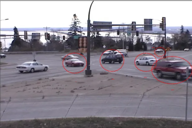
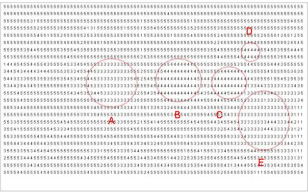
With the above definitions, the motion diagram showing the motion status of each block computed from block matching can be illustrated. The following three figures, Figure 2-3, 2-4, 2-5, obtained from MATLAB simulation, give an example of how the tracking algorithm detects the motion of the vehicles. Figure 2-5 has a dimension of 90×24 blocks and each element represents the motion status of that corresponding block. The red boxes in Figure 2-5 represent the same vehicles as in Figure 2-3. It can be seen that vehicle motions for these vehicles are mostly accurately identified. For example, vehicles A and E have mostly motion status of 3 for the blocks corresponding to the vehicle in the image. Practically, the number of a continuous region of 3s is also a good measure of the size of the vehicle in the image. Here, the red box A actually represents two vehicles due to merging. Vehicles B, C and D have mostly motion status of 4 for the blocks and the number of 4’s can also be looked as a good indication of the size of the vehicles. The left-most white vehicle and a few other vehicles beside B (refer to Figure 2-3) have no motion since they were waiting for the traffic signal. So, the motion status for these vehicles should be 5, which is the case as shown in Figure 2-5. But note that there are some noisy motion detections, which happened to the background blocks since the background is quite uniform and block matching computational might have made wrong decisions. And this noisy motion detection also happened to the vehicle E. The wrong decision could be partially corrected at the software part of the tracking algorithm, which will be discussed in Chapter 4. From this motion diagram the vehicles can be extracted using motion status and then tracked. 2.5 Step 3: Transmission of Motion Vectors to PC

After block matching computation, motion vectors are transmitted to the allocated buffer of the interface unit, which is a demo-kit included in original Micron image sensor system. Then by calling the software routines designed for the sensor system (the software is coded in C++) in a host PC, the motion vectors could be transmitted to the PC via a high-speed USB 2.0 port that connects the hardware sensor system and PC. We currently use MATLAB in a host PC to receive the motion vectors and post-process them. Section 3.4 gives more details on this.

2.6 Step 4: Vehicle Tracking In Software

Once the motion vectors are transmitted to the PC, they are processed by the MATLAB software to track vehicles. Therefore, the vehicle tracking software is developed in MATLAB. Briefly, the software tracking algorithm consists of two main components that are blob extraction and blob association. Referring to the example presented in section 2.4.1, the vehicle could be found by detecting a continuous region that contains elements of the same motion status. This kind of region is called a blob and the task of blob extraction is to find the blobs and extract their information such as position and size. Then the other component, blob association, is utilized to associate the blobs extracted by two consecutive blocking matching computations. This process goes on to keep tracking the vehicles. The details will be discussed in Chapter 4.

Figure 2-3: A traffic image captured at an intersection (frame N-1)

Figure 2-4: A traffic image captured at an intersection (frame N)

A B C

D

Figure 2-5: Block motion of frame (N-1) with respect to frame (N) 2.7 Comparison with Conventional Tracking Algorithm

In this section, the proposed tracking algorithm is qualitatively compared to the conventional ones in [4][5][6]. Both algorithms adopt the video based tracking approach. That is, the inputs to the tracking algorithm are image frames at different time instants. Regarding the difference in general, motion detection in [4][5][6] is object-based, in contrast to block-based motion detection for the proposed tracking algorithm. [4][5][6] rely on background subtraction and then thresholding to identify vehicle objects. Using the terminology, these objects are called blobs [4]. The blobs can be extracted from the difference image using a contour following algorithm [4]. It does so for two consecutive image frames N-1 and N, so that these two difference images are compared to identify the blob motion. To do that, it adopts a graph optimization approach. The blobs in each difference image is represented as a graph and the two consecutive graphs are optimized to find the best matching of the blobs in terms of minimum total size change with respect to the two consecutive difference images. After this, blob motion data processing and Kalman filtering are used for prediction of the motion. Figure 2-6 graphically illustrates how the conventional tracking algorithm works for the vehicle tracking.

This section identifies several disadvantages of the conventional tracking algorithms and explains the difference from the proposed tracking algorithm. First, the background subtraction involves a static background image, but the background may keep changing, which is not well addressed even with dynamic background updates [4]. Next, the image frame after background subtraction (the difference image) is thresholded to obtain a binary image. The threshold value has to be obtained by background training and is set to the absolute maximum fluctuation of pixel values (range from 0 to 255, for instance). This involves manual setting and could

introduce undesirable noise [4]. In contrast, the proposed approach of block matching does not require a static background image and the background change has negligible effect for block matching even when the frame rate is low. This makes the proposed tracking algorithm more robust and environmental changes that include weather variations.

Figure 2-6: An illustration of conventional tracking algorithms

Second, after thresholding the image is a binary digital image and only objects (blobs) are preserved in the image. Note that the pixel data information is now lost and all known is that whether each pixel corresponds to background or object. But in the proposed tracking algorithm, the rich pixel data information is kept and intentionally used for block matching whereas all pixels are thresholded to obtain a binary image in [4]. This makes the block matching algorithm potentially more accurate in terms of identifying the moving object since it is based on pixel value difference instead of size difference [4] in graph optimization of conventional tracking algorithm.

Third, the outputs of block matching are motion vectors, which can not only be used to extract the blob in the current image frame but also used to predict the position of the blob in the next image frame. Thanks to the motion vectors, the task of vehicle tracking simplifies to the association of blobs based on the amount of overlap between the blobs at the predicted position

(obtained from the former block matching) and the blobs at the measured position (obtained from the later block matching). Also, blob position prediction using motion vectors is much simpler and saves more computational time than Kalman Filtering based prediction in conventional tracking systems [4].

Fourth, the block matching algorithm in the proposed tracking system is more complicated than graph optimization in conventional tracking algorithm from algorithm point of view and typically takes longer computational time. For example, block matching computation is in the order of minutes in MATLAB simulation. This means that the proposed tracking algorithm can not be applied in real applications if it is implemented using a software approach, such as using MATLAB in a general purpose PC or a simple micro-controller. On the other hand, the block matching algorithm is well suited to hardware implementation. Therefore, in terms of implementation, most of the computation for the proposed tracking algorithm is done in hardware part, which is much faster than software implementations.

Overall, combined hardware implementation of the proposed tracking algorithm and simple processing steps of the software part clearly give a great timing advantage for vehicle tracking. This makes high-frame rate and real-time vehicle tracking feasible.

2.8 Summary

This chapter provides an overview of the processing flow of the proposed vehicle tracking system. The core of the tracking algorithm, motion estimation based on full-search block matching, is discussed and illustrated.

Chapter 3

Hardware Design of Motion Estimation Algorithm

3.1 Introduction

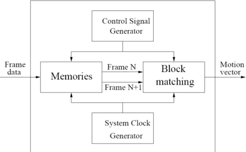
This chapter presents the design details of the hardware processor which implement the block matching algorithm to process the captured frames and output the motion vectors, which corresponds to step 2 in section 2.4. The hardware processor consists of four function blocks that are memories, a block matching module, a control signal generator and a system clock signal generator, as shown in Figure 3-1. The hardware processor is implemented using digital circuits for better design efficiency compared to analog circuits. We follow the four steps below to design the hardware processor. Firstly, Verilog code [18] is written for the overall hardware processor. Secondly, a Cadence CAD (Computer Aided Design) tool, NClaunch [19], is invoked to simulate the codes to verify the correct operation of the logic. Thirdly, another Cadence tool called Encounter RTL (Register Transfer Level) Compiler [20] is used to automatically synthesize the Verilog codes to circuit schematics. At last, the layout of the designed circuits is generated using the Cadence SOC (System-on-Chip) Encounter place and route [21]. The hardware processor is designed with the commercial IBM 0.13µm technology [22].

Figure 3-1: The hardware processor for motion estimation 3.2 Timing Budget

The core of the tracking algorithm, motion estimation based on block matching, requires heavy computations, i.e. a huge number of subtractions (refer to Section 2). Whether the tracking system can achieve real-time operation critically depends on the computational time of the block matching algorithm. If the algorithm is implemented in software, for example in MATLAB on a PC [23], the computational time is in the order of minutes for M = 288, S = 352, n = p = 8

(referring to section 2.4 for the definition of the parameters) and each pixel being a gray scale 8-bit integer. Therefore, if the proposed algorithm relies on software implementation, it has a much larger computational time than conventional tracking algorithms [4] [5] [6], therefore making frame rate for vehicle tracking even lower. However, if it is implemented in customized hardware, the block matching can be completed in much less time. The following sub-section discusses the timing budget of the tracking system to find out whether the processing speed of hardware processor meets the requirement of real-time operation.

3.2.1 Time of Frame Transmitting

Referring to the tracking system diagram in Figure 3-1, the first hardware part is the image sensor. But it has to be high-throughput to minimize the latency when outputting data (the data is pixel values of the image). In the proposed tracking system, the commercial image sensor, the MT9V111 sensor from Micron Technology [15], runs at a frame rate of 30 frames/second with resolution of 352×288 pixels. The master clock is 27 MHz and the output format is 8-bits parallel. That means each cycle of vehicle tracking has to finish within 1/30=33.33 milliseconds (ms) for real-time operation. As provided in the data sheets of the image sensor [15], the amount of time taken to transmitting a frame, whose resolution is 640×480, to the buffer is 63.92ms in the case that the master clock is 12 MHz. Note that the time for transmitting every pixel should be the same, which is one clock cycle. Therefore, the transmitting time of one image frame in the proposed tracking system could be approximately calculated by a linear solution as follows: 63.92 × 12/27 × (352×288) / (640×480) = 9.37ms. This leaves 33.33-9.37=23.96ms for motion estimation based on block matching. Note that there is no need to consider the time the software part takes because the processing of software part is independent from the hardware part, which is described in section 3.4 in detail.

3.2.2 Time of Block Matching

Whether the block matching computation in the proposed tracking algorithm can finish within such a time, 23.96ms, is next considered. In our processor design, in addition to the sensor master clock which is 27MHz, another clock of 333MHz is provided (the period time is 3 nanoseconds) for block matching computation itself in order to speed up the processing. This clock is determined after extensive simulations of the transistor-level circuits in each pipeline stage as described next. In the processor design, this clock is switched in after the current image frame is received and stored in the memory.

Typically, to improve hardware throughput, pipelining technique can be used at the expense of extra hardware design. One possible pipelining technique for block matching without incurring much extra hardware is called the systolic array processing technique [24]. In this approach, n×n adder circuits for block matching computation are used. Referring to the size of search area discussed in the section 2.4, the total number of additions (or subtractions) for one block matching is (n+2p) × (n+2p). Therefore, the total execution time (TET) for one block matching in this case would be approximately estimated (M=352, S=288, n=8, p=8) [28] as follows [25]: TET = (n+2p)×(n+2p)×(M×S)/(n×n)×clk = 24×24×(352×288) / (8×8) ×3 nanoseconds = 2.73ms

Note that each addition (or subtraction) takes one clock period. Thus, it can be seen that the execution time for block matching would easily meet the requirement of 23.96ms in order to achieve 30 frames/second vehicles tracking. Moreover, the rest 21.23ms (23.96-2.73=21.23ms) means that it is possible to increase the frame rate or more processing can be added in the hardware part if needed. However, the processing speed of software part may limit the frame rate.

3.3 Design Details of Hardware Processor

This section presents the details of how to design the hardware processor for the tracking system. As described in section 2.2, the hardware part consists of three components that are image sensor, hardware processor for motion estimation and interface unit. In the commercial Micron image sensor system, the sensor-head, which holds the lens and sensor core chip, and the demo-kit, which is used to transmit the image to the computer via a USB interface are included [17], as shown in Figure 3-2. Therefore, the main task is to design the hardware processor motion estimation.

Figure 3-2: Commercial Micron image sensor system 3.3.1 Memory Design

Since the image sensor captures and outputs images frame by frame and the block matching uses two consecutive frames for processing, two stacks of memories are needed to store the frames N and N+1.

To design the memory, the Artisan Standard Cell Library in IBM 0.13μm technology [26] is used. The SRAM Generator in the library is used to create instances of memory whose parameters meet the requirement. Figure 3-3 that is provided by the document of User Guide [26] shows every pin in the Synchronous Single-Port SRAM. The function of the memory is controlled by two inputs CEN and WEN. When the signal of CEN is high, the memory stays in the mode of standby. Then the address inputs are disabled and the data stored in the memory is retained, therefore memory cannot be accessed for new reads or writes. Data outputs remain stable. When both CEN and WEN are low, the memory stays in the mode of writing. The data on the data input bus, D[n-1:0], is written to the memory location specified by the address bus, A[m-1:0], and is driven through to the data output bus Q[n-1:0]. When CEN is low and WEN is high, the memory stays in the mode of reading. The data on the data output bus Q[n-1:0] takes

that of the memory location specified on the address bus A[m-1:0] and is read (by other external components).

The number of pixels in one image frame is 352×288=101,376, within 216 and 217, which means that the address bus A has to have at least 17 bits. However, referring to the User Guide [26], the maximum number of words that one block of memory could store is 16384=214. It is far from enough to store one frame, hence seven memory blocks are needed in order to store the entire frame. In the design, 14 out of the 17-bit address bus, A[13:0], specify the locations of pixels. The rest three bits are used as select signals to control a multiplexer to access one of the seven memory blocks. For example, suppose a 17 bit address, 101-01100111110010, is sent into the memory stack. The first three bits, 101 (equal to 5 in decimal), control the multiplexer to access the sixth memory block. Then the rest 14 bits are provided as an address to this memory block for writing or reading the data.

Figure 3-3: Synchronous Single-Port SRAM Diagram 3.3.2 Block Matching Algorithm Implementation

This section presents a VLSI architecture for implementing motion estimation based on full search block matching algorithm (FBMA), as described in reference [24]. Figure 3-4 shows the overall system architecture consists of three main functional blocks that are a systolic array combined with shift register arrays, a best match selection unit, and a control unit. The pixel data of the reference block and search area enters the systolic array serially from the input pins R and S. Then the output of the systolic array, the mean absolute difference (MAD), is sent into the best match selection unit to find the smallest value and output the motion vectors corresponding to that MAD value. The whole processing flow is synchronized by the control unit. Next, we detail on the design of each functional block.

A. Systolic Array Structure

The systolic array is constructed by n2 _{processing elements (PE}

i, j), (n-1) shift register arrays

(SRAi), and an n-input adder, as shown in Figure 3-5 [24]. The pixel data of the reference block

are serially delivered into the R input bus while the pixel data of the search area are serially fed into the S input bus. Once they are shifted to the correct locations, the PE’s of every column calculates the partial sums of the absolute differences in parallel and then sends them to the n-input adder to compute the MAD value of block matching for each candidate block. Since the

number of pixels of the reference block, n2, is less than that of the search area, (n+2p) 2, before the first search pixel arrives at the PE1, 1, all the reference block data {R (i, j) | 1≤i, j≤n} have

been shifted to and stored in all the PE’s, respectively. PEi, j store R (i, j) for i, j = 1~n until the

full-search block-matching is finished. Therefore, there are two clock signals, i.e., clk and clkr.

clkr is used to control the shift operation of the reference block data to PE’s. The clkr is

generated in the control unit (shown in Figure 3-4) and it provides n2 (the number of PE’s) clock periods to shift all the reference pixels to all PEs (as last, the first reference pixel is stored in PE1, 1). clk is the system clock, which is used to shift the pixels of the search area into the PEs as well

as control the internal addition (or subtraction) of all PEs.

Figure 3-4: The hardware architecture to implement FBMA

Note that though the data flow of the architecture is serially in and serially out, the inherent spatial parallelism and temporal parallelism are fully exploited in the computation to speed up the processing [24]. From the definition of MAD in Section 2.4, there are n×n additions of pixel absolute difference for every MAD value. It takes n×n clock cycles if no parallel processing is used, which make the computational time of motion estimation much longer. However in this architecture, the two-dimensional systolic array and shift register arrays, which include (2p-1) shift registers, are used to achieve the goal of parallel processing while avoiding multiple data inputs.

Assume the first search area pixel shifting in the array is S (1, 1). In the first clock cycle, it is shifted to PE1, 1 while S (1, n) is in PE1, n. That means the first row data of the first candidate

block have been shifted into the PE1, j, j = 1~n and their absolute difference (AD) values AD1, j, j

= 1~n are calculated simultaneously. In the second clock cycle, these values are shifted up and added with the AD2, j, j = 1~n calculated by the PE2, j, j = 1~n, which process S (2, j), j = 1~n, the

second row data of the first candidate block. Thus, the n sums AD1, j + AD2, j, j = 1~nare

obtained. Note that in the same clock cycle, the PE1, j, j = 1~n get S (1, j), j = 2~n+1, which are

the first row data of the second candidate block. Similarly, in the third clock cycle, the sums AD1, j + AD2, j + AD3, j, j = 1~n for the first candidate block, the sums AD1, j + AD2, j, j = 2~n+1

for the second candidate block, andAD3, j, j = 3~n+2 for the third candidate block are calculated.

By following this parallel processing pipeline, after n clock cycles, the parallel adder adds the n column partial sums AD1, j + … + ADn, j, j = 1~n to obtain the first matching result MAD. In

clock cycle n+1, the second MAD value outputs, and the third one in clock cycle n+2, and so on. This means one MAD value is computed in a single clock cycle, which improves the throughput.

B. PE Design

Figure 3-6 illustrates the block diagram of PEi, j [24]. Each PE is constructed by an absolute

difference calculator (ADC), an adder, and four shift registers (L1~ L4). ADC computes the AD

between the search pixel shifted from the left-neighbor PEi, j+1 (or from SRAn-i) and the reference

pixel R (i, j) stored in the L2. The AD value delayed one clock period by L3 is added to the result

shifted from the down-neighbor PEi-1,j. Then the sum is passed to the up-neighbor PEi+1, j after

being delayed one clock period by the L4. The L1 implements an independent path for the

shifting of the search pixel. Note that different with L1 L2 L3, whose widths are 8 bits, the width

of L4 is (8+k), while i=2k since the maximum sum of AD values of each column is i×28=2k+8.

Figure 3-6: Block diagram of PEi, j

C. Shift Register Arrays

Depending on several factors, such as the vehicle size, the vehicle speed, or the frame rate, the size of the search area could be set larger or smaller. Therefore, the length of each SRA is designed to be programmable to meet the requirement of the changeable size of the search area. Figure 3-7 shows the diagram of the programmable SRA that provides four sizes to the search area [24]. In the design, n=8, p=5, 6, 7, or 8, so the dimensions of the search area could be 18, 20, 22, or 24, respectively. 15 shift registers are separated to four groups of 9, 2, 2, 2 registers by four control blocks SW1 ~ SW4. SWn, controlled by the signal cn generated in the control unit, is

a switch used to open or close the path between the groups. For example, if the desirable size of the search area is 22, then the control signal c1c2c3c4=1110. In this case, SW3 blocks the last

group of 2 shift registers, and the length of the SRA is thus 9+2+2=13.

Figure 3-7: Block diagram of the shift register array (SRAi)

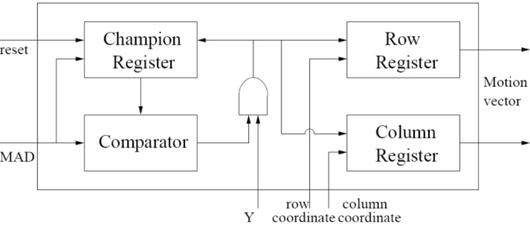
D. Best Match-Selection Unit

Figure 3-8 shows the block diagram of the best match-selection unit [24]. The champion register is used to store the smallest MAD value from the block matching computation. The champion

register is connected to the comparator to compare to the new MAD value for the following candidate block. If the coming challenger is smaller and the input signal Y indicates that the coming MAD is valid, it will replace the current champion in the champion register and the corresponding motion vector will be recorded in the row and column registers. Otherwise, the registers will be disabled and the previous data remains locked. Before the next block matching computation for a new reference block, a reset signal is sent to initialize the champion register to a large value (as motion estimation looks for minimum MAD).

Figure 3-8: Block diagram of the best match-selection unit E. Control Unit

Figure 3-9 shows the block diagram of the control unit [24]. The row and column counters provide the coordinates of the candidate blocks. Moreover, to prevent the invalid candidate blocks from resulting in the wrong motion vectors, the signal Y is generated to check if the coordinates corresponding to the current MAD value is valid or not. As shown in Figure 3-10, the first valid MAD value is obtained when the shifted search pixel reaches the coordinates (n, n) and PE (1,1) in the systolic array. Besides, the control code generator produces the control signals c1 ~ c4 to change the length of the shift register arrays as described in last sub-section. It

is specified by the two parameters, n and p, which are preset by users.

As described in the design of the systolic array, a special clock signal clkr is needed to control

the shifting of the reference pixels. It is produced by the reference clock generator which has a counter for counting the number of clock periods of the system clock clk. The clkr equals to clk

Figure 3-9: Block diagram of the control unit

Figure 3-10: The regions of valid and invalid MAD values 3.3.3 Design of Control Signal Generator

The function of the control signal generator is to synchronize and control the timing within all parts of the hardware processor. Figure 3-11 shows the structure of the generator.

Referring to the data sheets of the Micron image sensor [15], there are 26 pins for the image sensor outputs. Among the 26 output pins, the 8-bit pixel output, the pixel clock, the frame valid signal, and the line valid signal are used in our hardware processor. The timing of these signals is shown as Figure 3-12. The rising edge of the frame valid signal means the captured frame is ready to output and the frame pixel data is transmitted when the frame valid signal is high. Since the size of the original frame captured by the sensor core is larger than the standard resolution due to blanking, the line valid signal is used to specify the valid pixel data in rows. During the high level of line valid, one row of pixel data of the image frame is transmitted.

Thus, both the frame valid and line valid signals control memories’ timing of either writing or reading data. As the main component of the control signal generator, SRAM controller generates not only the control signals of CEN and WEN, but also the memory addresses for writing and reading data. In the case that the frame valid signal is high and line valid signal is also high, both the CEN and WEN are set to low to make the SRAM stay in the mode of writing data and a counter produces the corresponding addresses to the input bus A of the SRAM. Otherwise, when the line valid signal flips to low, the invalid pixel data is blocked from SRAM. In this case, the CEN is set to high and mode of SRAM to standby. Meanwhile, the address generation is halted until the next rising edge of the line valid signal comes. Since the single-port SRAM does not allow writing and reading in the same time, the wanted data cannot be read until the whole frame is stored, which is the time of the falling edge of the frame valid signal. The dual-port SRAM could solve the problem since it has two ports for simultaneous reading and writing, which could help reduce the overall processing time of motion estimation. However, it was not adopted in the design since its memory size is only half of the single-port. On the other hand, the reduction of processing time is not significant even with dual-port SRAM [26].

Figure 3-11: Block diagram of the control signal generator

When the frame valid signal is low, the SRAM stays in the mode of reading data by setting the CEN to low and the WEN to high. Note that when reading data from the memory to supply into the block matching hardware, the faster clock of 333MHz is switched in. Suppose that two consecutive frames have already been stored in two SRAM stacks, a counter generates the addresses of the reference pixel data for frame N while another one is responsible for the addresses of the search pixel data for frame N+1. Then the two sets of pixel data are sent to the systolic array serially as described before. To be efficient, the two memory stacks alternatively store the new coming frame. Assume that the frame N is stored in SRAM1, the SRAM2 is accessed to store the frame N+1, and the search pixels are read from it while the reference pixels are read from SRAM1. Then next time, SRAM1 gets the frame N+2 and this time SRAM2 supplies the reference pixels. The data access scheme could be easily implemented by

multiplexers, as shown in Figure 3-13. For instance, suppose that Dout is connected to D1, AA to

A1, AB to A2, O1 to S, and O2 to R (AA, AB denote address bus inputs). Once the rising edge of

the frame valid signal comes, the connections change to that Dout to D2, AA to A2, AB to A1, O1

to R, and O2 to S.

As described in last section, every time before the computation of block matching for one candidate block, a reset signal is needed to initialize champion registers and counters in best match selection circuit. Note that in theory every computation of block matching takes (n+2p)×(n+2p) clock cycles (576 if n=p=8). Therefore, a reset occurs after every this number of clock cycles.

Referring to the sensor data sheets [15], the pixel clock, the frame valid and the line valid signals are used to control the demo kit to store valid pixels of image frames. In our design, the hardware processor for motion estimation is inserted between the sensor and the demo kit. With the new system, the motion vectors computed from block matching are stored in the buffer instead of pixels of image frames. To be able to re-use the commercial demo-kit, different control signals that are compatible to the motion vectors outputs need to be generated. How to generate these signals is explained as follows. In the same way as producing the reset signal, a new pixel clock is generated at the ending time of every block matching (when the motion vectors are stored in the result registers). Since the valid time for outputting motion vectors is when the block matching finishes computation, which is the same time when the original frame valid signal is low, the new frame valid signal is obtained by simply inverting the original one. The new line valid signal is the same as the new frame valid signal because different from the original image pixels outputs, there is no invalid motion vectors output. The timing diagram of the new control signals is shown in Figure 3-12.

3.3.4 Design of System Clock Signal Generator

According to Micron image sensor data sheets [15], the pixel output format chosen is “YCbCr”, which uses two bytes to represent a pixel. The full-search block matching algorithm only needs the grayscale value, i.e., the data of Yi, which is in the second byte. Therefore, a writing clock

signal is generated to pick up Yi from the sensor output and then write it into SRAM. The clock

period of this clock is double of the sensor’s master clock period (called pixel clock in Micron image sensor system referring to Figure 3-2) [15]. Moreover, as described in Section 3.2.2, another clock signal with frequency 333MHz is provided to read data from SRAM for block matching computation. This means that two different clocks are used when reading from and writing to SRAMs. From Figure 3-3 there is only one clock input pin in SRAM. Hence, the function of the system clock signal generator is to combine the two different clocks to produce a system clock that is connected to SRAM’s clock input.

Figure 3-12: The original and new buffer control signals

Figure 3-13: Alternative SRAM switching to store new frame data 3.3.5 Entire Hardware Part

For the proposed tracking system, Figure 3-14 shows the diagram of entire hardware part. Compared to the original Micron image sensor system shown in Figure 3-2, a hardware processor is designed and assembled into the original sensor system.

3.4 Interface Unit

In the commercial Micron image sensor system, the frames captured by the sensor head is stored in the buffer of demo-kit and transmitted to a computer with a USB 2.0 port (refer to Figure 3-2 and 3-14) [17].

However, as described in section 3.3.3, in the proposed tracking system the data that should be stored in buffer is motion vectors (refer to Figure 3-14). Also as discussed in Chapter 2, the hardware in Figure 3-14 takes care of the tasks 1 to 3 whereas task 4 is decided to be implemented in the traditional software approach. Therefore, the motion vectors stored in the buffer of demo kit needs to be sent to a PC for further processing.

Currently, task 4 is implemented in the commercial software MATLAB [23] in a host PC. The Micron Imaging Device Library [17] provides a device independent API (Application Programming Interface written in C/C++ programming language) for seamless device control and data transport. By calling these APIs, the motion vectors can be read into MATLAB from the buffer. Figure 3-15 presents the pseudo-codes of how to control the sensor system to obtain the motion vector data from the buffer.

1. Find a camera connected to the computer 2. Allocate the buffer to store the data 3. Turn on the camera

4. Grab a frame of data and store it in the buffer

5. Send the data to MATLAB workspace through the pointers of API 6. Turn off the camera and free the buffer

Figure 3-15: Pesudo-code for reading data from the buffer 3.5 Logic Simulation Result

To verify the design of the hardware processor, Verify code is written for the hardware processor and simulated in NClaunch, a CAD Tool of Cadence [19]. The simulation results verify the correction operation of the hardware processor. Figure 3-16 presents only a glimpse of the simulation results. The output data “HDQ” is the smallest MAD value from every block matching computation, and “HDC” and “HDR” are the corresponding coordinates, also the motion vectors. The waveform of the new buffer control signals of frame valid, line valid and pixel clock are denoted as “NewFV”, “NewLV” and “NewCLK” (refer to Figure 3-11).

3.6 Summary

This chapter discusses the timing requirements of the hardware processor and presents the design details of every functional block in it. The entire hardware processor is coded in Verilog hardware description language and verified by simulation.

Chapter 4

Design of Software Part of the Tracking System

4.1 Introduction

This chapter presents the developed software program in MATLAB that is used to track vehicles by processing the motion vectors that are outputs from the hardware processor described in Chapter 3. The software here implement step 4 of the overall processing algorithm (refer to Figure 2-1). The software program consists of two sections that are bl