This is a repository copy of
Log-linear system combination using structured support vector
machines
.
White Rose Research Online URL for this paper:
http://eprints.whiterose.ac.uk/152833/
Version: Published Version
Proceedings Paper:
Yang, J., Ragni, A. orcid.org/0000-0003-0634-4456, Gales, M.J.F. et al. (1 more author)
(2016) Log-linear system combination using structured support vector machines. In:
Interspeech 2016. Interspeech 2016, 08-12 Sep 2016, San Francisco, CA, USA.
International Speech Communication Association (ISCA) .
10.21437/interspeech.2016-377
© 2016 International Speech Communication Association. Reproduced in accordance with
the publisher's self-archiving policy.
[email protected]
https://eprints.whiterose.ac.uk/
Reuse
Items deposited in White Rose Research Online are protected by copyright, with all rights reserved unless
indicated otherwise. They may be downloaded and/or printed for private study, or other acts as permitted by
national copyright laws. The publisher or other rights holders may allow further reproduction and re-use of
the full text version. This is indicated by the licence information on the White Rose Research Online record
for the item.
Takedown
If you consider content in White Rose Research Online to be in breach of UK law, please notify us by
Log-linear System Combination Using Structured Support Vector Machines
J. Yang, A. Ragni, M. J. F. Gales and K. M. Knill
Department of Engineering, University of Cambridge, Cambridge, UK
{jy308,ar527,mjfg,kate.knill}@eng.cam.ac.uk
Abstract
Building high accuracy speech recognition systems with limited language resources is a highly challenging task. Although the use of multi-language data for acoustic models yields improve-ments, performance is often unsatisfactory with highly limited acoustic training data. In these situations, it is possible to con-sider using multiple well trained acoustic models and combine the system outputs together. Unfortunately, the computational cost associated with these approaches is high as multiple decod-ing runs are required. To address this problem, this paper exam-ines schemes based on log-linear score combination. This has a number of advantages over standard combination schemes. Even with limited acoustic training data, it is possible to train, for example, phone-specific combination weights, allowing de-tailed relationships between the available well trained models to be obtained. To ensure robust parameter estimation, this paper casts log-linear score combination into a structured support vec-tor machine (SSVM) learning task. This yields a method to train model parameters with good generalisation properties. Here the SSVM feature space is a set of scores from well-trained individ-ual systems. The SSVM approach is compared to lattice rescor-ing and confusion network combination usrescor-ing language packs released within the IARPA Babel program.
Index Terms: system combination, structured support vector machines, speech recognition, keyword spotting
1. Introduction
Automatic speech recognition (ASR) systems generally require training on large amounts of data to achieve high accuracy. However, sufficient data cannot normally be guaranteed for many low resource languages. Automated approaches can be used to increase the amount of training data, such as synthe-sising speech with the known transcriptions [1] and using un-transcribed audio in semi-supervised training [2]. An alterna-tive solution to this problem is to use data from other languages to train a multilingual deep neural network (DNN) [3, 4] to produce more robust bottleneck features. Although these data augmentation schemes yield improvements [5, 6], performance is often unsatisfactory. Thus, a combination of multiple well trained systems might be preferred.
In general system combination approaches can be divided into two distinct groups, i.e. hypothesis combination and log-likelihood score combination. Recogniser output voting error
This work was supported by the Intelligence Advanced Research Projects Activity (IARPA) via Department of Defense U.S. Army Re-search Laboratory (DoD/ARL) contract number W911NF-12-C-0012. The U.S. Government is authorized to reproduce and distribute reprints for Governmental purposes notwithstanding any copyright annotation thereon. Disclaimer: The views and conclusions contained herein are those of the authors and should not be interpreted as necessarily rep-resenting the official policies or endorsements, either expressed or im-plied, of IARPA, DoD/ARL, or the U.S. Government.
reduction (ROVER) [7] and confusion network combination (CNC) [8] are typical examples of combining the hypotheses generated by different recognisers. In these approaches, differ-ent hypotheses to be combined are generated from separate de-coding runs on various systems. It is computationally expensive to run multiple passes of decoding, and the cost is even higher when speech recognition is an intermediate process, such as in keyword spotting (KWS) [9]. Thus, more efficient approaches based on log-likelihood score combination might be preferred. Here, the log-likelihoods from different systems are combined, and only a single decoding run is required.
Joint decoding [10] is a typical example of log-likelihood score combination, where the state (frame level) log-likelihoods of tandem [11] and hybrid [4] systems are linearly com-bined. The systems to be combined share the same hidden Markov model (HMM) topology and the combination weights are typically manually set. This makes joint decoding highly constrained. An alternative to combining frame level log-likelihoods is to combine segment level HMM log-log-likelihoods. This relaxes the frame level Markov assumption to the segment level, and synchronises systems at the phone (or word) level rather than frame. This relaxation also allows long-span depen-dency within the segments to be captured.
In [12], structured discriminative models are trained using the feature space based on phone log-likelihoods with the same context but different central phone generated by tandem and hy-brid systems. Small gains were observed from using additional log-likelihoods extracted from the same models. [13] exam-ines combination of hybrid and tandem systems with log-linear models, and applies learnt phone-specific combination weights to frame level joint decoding, achieving a small performance gain. [14] discusses model combination at sentence level, using system-specific combination weights. A more general frame-work was introduced by [15], where systems are combined at word level, and the word-specific combination weights are trained with the minimum Bayes risk (MBR) criterion. Another approach was investigated in [16]. However, these approaches are still limited as some words in decoding may not appear in training, especially in low resource language tasks.
The log-likelihood score combination approach is investi-gated in this paper. This approach is cast into a structured support vector machine (SSVM) [17, 18, 19] learning task to robustly estimate phone-specific combination weights. In this work, a more meaningful feature space is used, which is based on phone log-likelihoods from multiple systems, rather than us-ing extra phone log-likelihoods with the same context extracted from a single system. This paper also discusses assumptions applied in typical combination approaches, such as frame level and segment level lattice rescoring, and investigate what impact these assumptions have on system combination gains. To as-sess the impact of different approaches on a downstream task, KWS performance is also examined. All experiments are
car-INTERSPEECH 2016
ried out on the highly challenging IARPA Babel evaluation task. The paper is organised as follows. In section 2 different monly used combination approaches and the generation of com-plementary systems are discussed. The SSVM is introduced in section 3. Finally, experimental results and conclusions are pre-sented in sections 4 and 5.
2. System Combination
In standard decoding, the Viterbi algorithm is employed to find the best hypothesisWˆ. Given an utterance O, the decoding process can be described as:
ˆ W = arg max W n p(O|W)P(W)αo (1)
wherep(O|W)andP(W)are the likelihood and probability given by the acoustic (AM) and language (LM) models. αis the LM scale factor. In hypothesis combination approaches, such as ROVER [7], multiple decoding runs are required which is computationally expensive. Alternatively, a single set of lat-tices generated by one system can be rescored by using other systems. Then the hypothesis combination approaches can be applied to the lattices rescored by different systems. This type of approach can significantly reduce the computational over-head as the search space (or hypotheses) is given by the lattice. The rescoring process can be described as:
ˆ
W = arg max
W∈L n
p(O|W)P(W)αo (2)
whereW ∈ Ldenotes a possible hypothesis given by a de-terminised lattice. p(O|W)andP(W)are the likelihood and probability given by AM and LM, respectively, which might differ from the ones used to generate the lattice. This approach is referred to asframe level lattice rescoringin this paper.
A far more efficient way to rescore the lattice is to fix both the search space and phone segmentations, referred to as seg-ment level lattice rescoring. It can be expressed as:
( ˆW ,ρˆ) = arg max W,ρ∈L |ρ| Y i=1 p O(i)|wi P(W)α (3)
whereW,ρ ∈ Ldenotes a possible hypothesis and the corre-sponding segmentation given by a lattice, andp(O(i)|wi)is the
likelihood (corresponding to segmentO(i)with triphone label1
wi) given by an AM, which might differ from the one
generat-ing the lattice. |ρ|is the number of segments. By using loga-rithms, equation (3) can be rewritten as:
( ˆW ,ρˆ) = arg max W,ρ∈L ( 1 α T P|ρ| i=1logp O(i)|wi logP(W) ) (4)
This is a linear combination of log-likelihoods from a single system. Before introducing the SSVM approach, the possible ways of generating complementary systems (that make different errors) will be discussed in the following subsection.
2.1. Complementary System Generation
In system combination, it is assumed that the systems to be combined complement each other. The most commonly used approach to generating complementary systems is simply to train a number of independent systems with different
acous-1The following discussion on phonemic systems also applies to graphemic systems. Tandem PLP Pitch Bottleneck Filterbank Pitch Context Dependent Targets A AK CMLLR PLP Pitch Stacked Hybrid
Figure 1: Tandem and stacked hybrid systems. tic modelling techniques. These individual systems might use different front-ends, segmentations, dictionaries or decision trees [20, 21]. Figure 1 illustrates the framework of the tandem and stacked hybrid systems used in this work. In this frame-work, complementary systems might be generated, for example, by using different (unilingual or multilingual) data to train the bottleneck DNN, employing different input feature types, using different supervisions to train the transforms, semi-supervised AM training, or using different structures or activation functions for the bottleneck or hybrid DNNs. All these approaches lead to potentially complementary systems, but there is no theoretical guarantee, hence a number of experiments must be performed to select the optimal combination [20]. However, standard ap-proaches to assess how complementary individual systems are would involve multiple decoding runs which are time consum-ing. Alternatively, complementarity can be efficiently evaluated by the combination approaches based on lattice rescoring with different AMs. This is examined in the experimental section.
3. Structured Support Vector Machines
In its basic form, a support vector machine (SVM) is a linear classifier [22]. To classify observation sequencesOinto one of many possible sentencesW with a SVM, the simplest option is to map them jointly into a fixed dimensional representation
Φ(O, W). Unfortunately extracting fixed dimensional features from variable-length observation sequences and modelling the vast, unstructured, mostly unseen space of possible sentences is non-trivial [23]. Instead, a structured assumption is usually imposed on the label space making sentences to be variable-length sequences of finite vocabulary units such as words or phones. The variable-length issue is then delegated to those units by aligning them with observations to yield alignmentρ
dependent feature vectorsΦ(O, W,ρ). This serves the basis of structured discriminative models including SSVMs. Classifica-tion is performed by solving a semi-Markov inference problem [24]: ( ˆW ,ρˆ) = arg max W,ρ n αTΦ O, W,ρo (5)
Efficient inference can be performed if the search space in equa-tion (5) is constrained to fewer hypotheses encoded compactly in a lattice [25, 26]. Such lattices can be efficiently generated using standard HMM-based approaches [27]. It is simple to no-tice that the inference problem in equation (5) or its latno-tice based approximation includes equation (4) as a subproblem. This re-lationship will be explored in the rest of this section.
The key concept of SVMs is a margin defined as the dis-tance between the closest correct and incorrect class example [22]. For SSVMs this can be defined by:
M Wn,ρn, W,ρ;α,On =αTΦ On, W n,ρn −αTΦ On, W,ρ (6)
1899
where (Wn,ρn) and (W,ρ) are correct and incorrect
align-ments for observation sequenceOn. For a sequence classifi-cation task it is important to take into account loss,L(Wn, W),
as different alignments make different number of transcription errors. Training then consists of minimising the largest viola-tion of the loss-augmented margin [17]:
FLM(α) =−logp(α) + N X n=1 max W6=Wn n L(Wn, W)− M Wn,ρn, W,ρ;α,On o + (7)
whereN is the number of training examples, and[·]+ is the
hinge loss. W 6= Wn denotes any possible hypothesis that
differs from the reference Wn2. p(α) = N(µα, CI) ∝
exp − 1
C||α−µα|| 2
is the Gaussian prior with meanµα
and diagonal covarianceCI. The objective function in (7) can be efficiently solved by using the cutting plane algorithm [28]. In this work, the segmentations corresponding to the references are the most likely segmentations given by the HMMs. An alter-native approach to obtain optimal segmentations by using dis-criminative models is discussed in [17].
There are a number of possible forms for alignment de-pendent feature vectorsΦ O, W,ρ
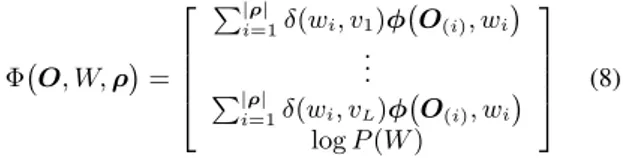
. Typically they consist of observation and transition features [26]. Observation features are extracted from variable-length observation sequences asso-ciated with units whereas transition features are extracted on transitions from one unit to another. One simple form is [29]:
Φ O, W,ρ = P|ρ| i=1δ(wi, v1)φ O(i), wi .. . P|ρ| i=1δ(wi, vL)φ O(i), wi logP(W) (8) where{vl}L
l=1denotes all possible phone units in the
dictio-nary. δ(·)is the Kronecker delta3. φ(O(i), wi)is the
obser-vation feature vector for segmentO(i). In general, this
fea-ture vector can be produced by using any approach capable of mapping variable length observation sequences to fixed length. It can be a first and higher order observation statistics tradi-tionally used with frame level models [30, 31]. Other ex-amples include score spaces [32, 33, 34] and event detectors [26, 16]. A simplest example is given in (4), where the mapping for a segment O(i) with labelwi is a log-likelihood, namely φ(O(i), wi) =
logp(O(i)|wi)
. This work employs a more general form, which consists of log-likelihoods from multiple AMs, rather than a single one. LetKbe the number of AMs, the observation feature vectorφ(O(i), wi)and the
correspond-ing phone-specific weights can be described as:
φ O(i), wi = logp1 O(i), wi . . . logpK O(i), wi ,αwi= α1wi . . . αKwi (9)
By setting the weights corresponding to an individual system to 1 and others to 0, the SSVM will retrieve the performance of segment level lattice rescoring described in (4). Moreover, by using these manually set weights in the prior, optimal weights can be learnt by using the large margin training criterion (7).
2Since segmentations are introduced, hypotheses having a different segmentation to the reference are treated as different to the reference.
3When segment label
wiis a triphone andvlis a monophone, in the delta function the context ofwiis stripped off.
This approach is adopted in the experiments, where the SSVMs are trained based on these priors with strong baselines.
4. Experiments
Different system combination approaches discussed in the pre-vious sections are examined in this section, with ASR and KWS performance presented. Experiments are performed on the Swahili and Javanese full language packs4released within the IARPA Babel program, which contain around 40 hours of transcribed conversational telephone speech data for training.
Approach Decoding # KWS # Standard 4 4 Rescoring (frame) 1 4 Rescoring (segment) 1 4
SSVM 1 1
Table 1: Resource requirements of different approaches. A combination of 4 joint decoding [10] (tandem and hybrid) systems is examined. Table 1 lists the number of decoding and KWS runs for different combination approaches. As discussed in section 2, for the “Standard” combination approach, 4 passes of joint decoding are run to generate 4 sets of hypotheses. Then CNC is used to combine these hypotheses. This approach also requires 4 KWS runs, with the final KWS result obtained by merging the 4 KWS posting lists. For the frame and segment level lattice “Rescoring” approaches, only 1 decoding run is re-quired to generate 1 set of lattices which can then be rescored as discussed in section 2. It is worth noting that rescoring may use different pruning settings to the standard decoding. Similar to the standard approach, 4 KWS runs are performed based on these 4 sets of rescored lattices, and finally the 4 KWS posting lists are merged. In the “SSVM” approach discussed in sec-tion 3, only 1 decoding run is required to generate the lattices. Then the lattices are rescored by using the log-likelihoods from different systems (those form the joint features) and the learnt combination weights for the SSVM as described in equation (5). Based on the rescored lattices, only 1 KWS run is required.
4.1. Experiments on Swahili
Table 2 gives the word error rates (WER) on the Swahili dev set. S1, S2, S3 and S4 are joint decoding systems, which combine the tandem and hybrid log-likelihoods at frame level. S1, S2 and S3 differ in the structure of the bottleneck DNN5: they use 26, 39 and 62 dimensional bottlenecks respectively. S4 uses 39-d bottleneck and semi-supervised training. Lattices generated by the S1 system are used for rescoring experiments. For example, the SSVM combination weights are trained based on lattices generated with a bigram language model (LM). In decoding, bigram lattices are rescored with a trigram LM and the scores from the systems to be combined. In the first block (from row 1 to 4) of Table 2, all the numbers are confusion network (CN) results. The second block lists the CNC results.
Since S1, S2, S3 and S4 use different model structures and are trained with different training technologies, they may com-plement each other. Moreover, these 4 joint decoding systems have comparable performance (see “Standard” column), this makes a good combined performance possible, and experiments show that the CNC result (43.5%) is much better than the result of any individual system. For the system combination results,
4Swahili IARPA-babel202b-v1.0d, Javanese IARPA-babel402b-v1.0a.
System Standard Rescoring SSVM Frame Segment Manual Train S1 44.7 44.8 45.0 43.8 43.1 S2 45.6 45.3 45.7 S3 44.6 44.6 45.1 S4 44.7 44.7 45.5 CNC 43.5 43.5 43.7 – – Time (hrs) 19 7 10 9 9
Table 2: WER performance on Swahili (202) Eval15 dev set.
System Standard Rescoring SSVM Frame Segment Manual Train S1 0.543 0.543 0.541 0.559 0.558 S2 0.537 0.535 0.539 S3 0.540 0.543 0.545 S4 0.544 0.543 0.535 PM 0.570 0.566 0.561 – – Time (hrs) 25 14 15 3 3
Table 3: MTWV performance on Swahili (202) Eval15 dev set. frame level lattice rescoring achieves the same result (43.5%), indicating that the S1 lattices contain good sets of hypotheses enabling equation (2) to approximate equation (1) accurately. Segment level lattice rescoring gives a worse result (43.7%), suggesting the segmentations from S1 lattices are not optimal for S2, S3 and S4. Since the rescoring approaches only need 1 decoding run, the complementarity of individual systems can be efficiently evaluated by these approaches. For the SSVM, with manually set weights6, the performance (43.8%) is worse than the CNC result of the “Standard” approach. Phone-specific trained weights yield a0.7%absolute performance gain in the SSVM to43.1%, which is better than the “Standard” CNC re-sult43.5%. As seen in Table 2, the frame level lattice rescoring takes slightly less time than SSVM due to the time consuming generation of log-likelihood scores.
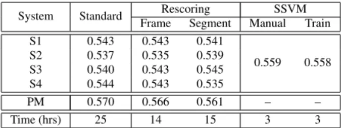
Table 3 gives the KWS performance for the different combi-nation approaches, measured by maximum term weighted value (MTWV) [35]. The “Standard” posting list merge (PM) ap-proach (that merges the posting lists generated by S1, S2, S3 and S4) achieves the best result (0.570). However, this ap-proach is highly inefficient as 4 decoding and 4 KWS runs are required. More efficient approaches based on lattice rescoring can be used, with 1 decoding and 4 KWS runs. Although frame and segment level rescoring yield accurate approximations to frame-level inference in terms of WER, these approaches dis-play sensitivity in terms of KWS. They obtain worse PM re-sults, i.e. 0.566 and 0.561 for the frame and segment levels. These results are better than any result of the individual sys-tems S1, S2, S3 and S4, given in the “Standard” column. Since 4 KWS runs are highly inefficient, the SSVM combination ap-proach can also be adopted, where only 1 KWS run is required. As shown in Table 3, this is 5×faster. Although for both the manually set and trained weights, the performances are worse than the “Standard” PM result, the “SSVM” results (0.559 and 0.558) are much better than the “Standard” results of the indi-vidual systems. SSVM training does not help for KWS, as it aims to reduce overall classification errors but gives high dele-tion error rate. In conclusion, the suggested KWS approach is a SSVM with manually set weights, since, compared with other schemes, this approach is much more efficient and has much better performance than any individual systems.
6These system-dependent weights are(α
4, α 4, α 4, α 4)for S1, S2, S3 and S4, whereα= (0.25,1.0)corresponding to tandem and hybrid.
System Standard SSVM Manual Train J1 53.0 52.6 52.4 J2 53.6 J3 54.6 J4 59.8 CNC 52.4 – – Time (hrs) 49 13 13
Table 4: WER performance on Javanese (402) dev set.
System Standard SSVM Manual Train J1 0.451 0.461 0.459 J2 0.446 J3 0.420 J4 0.362 PM 0.463 – – Time (hrs) 40 8 8
Table 5: MTWV performance on Javanese (402) dev set.
4.2. Experiments on Javanese
It is time consuming to generate multiple complementary sys-tems using different model structures or modelling techniques. A simple way to create possible complementary systems is to use different bottleneck features, and this approach is examined on the Babel Javanese data. The systems J1, J2, J3 and J4 pre-sented in Table 4 only differ in the bottleneck DNNs, which are trained on different data sets: J4 – unilingual; J3 – 11 lan-guages7; J2 – 24 languages8; J1 – 24 languages with fine-tuning to Javanese. These individual systems can be relatively easily generated, but the results in Table 4 show that these systems are not good examples of complementary systems. The CNC result (52.4%) is not significantly better than the J1 result (53.0%). These systems have high deletion rate. The SSVM can only match the CNC result. This indicates that it is hard for SSVMs to take advantage of extra features from other systems, when in-dividual systems are not complementary. However, the SSVM with trained weights is the most efficient and effective approach. For the KWS results shown in Table 5, the SSVM with manually set weights9, has a comparable result (0.461) to the
PM (0.463), but only 1 KWS run is required by the SSVM, and only needs1/5of the time used by the standard approach.
5. Conclusions
This paper has examined the impact of different combination approaches on both the ASR and KWS performance. The pro-posed SSVM combination approach, that only needs 1 decod-ing and 1 KWS run, can achieve good ASR and KWS perfor-mance very efficiently. However, training the SSVM weights gives worse KWS performance which needs to be investigated further.
7Cantonese IARPA-babel101b-v0.4c, Assamese babel102b-v0.5a, Bengali babel103b-v0.4b, Pashto babel104b-v0.4aY, Turkish babel105b-v0.4, Tagalog IARPA-babel106-v0.2f, Vietnamese IARPA-babel107b-v0.7, Haitian Creole babel201b-v0.2b, Lao babel203b-v3.1a, Tamil IARPA-babel204b-v1.1b, Zulu IARPA-babel206b-v0.1d.
8Plus Kurmanji Kurdish IARPA-babel205b-v1.0a, Tok Pisin IARPA-babel207b-v1.0b, Cebuano IARPA-babel301b-v2.0b, Kazakh IARPA-babel302b-v1.0a, Telugu IARPA-babel303b-v1.0a, Lithuanian IARPA-babel304b-v1.0b, Swahili IARPA-babel202b-v1.0d, Guarani IARPA-babel305b-v1.0a, Igbo IARPA-babel306b-v2.0c, Amharic IARPA-babel307b-v1.0b, Mongolian IARPA-babel401b-v2.0b, Ja-vanese IARPA-babel402b-v1.0b, Dholuo IARPA-babel403b-v1.0b
9Since the individual systems do not have comparable performance, the system-dependent weights are set to(0.6α,0.3α,0.1α,0).
6. References
[1] M. J. F. Gales, A. Ragni, H. AlDamarki, and C. Gautier, “Support vector machines for noise robust ASR,” inProceedings of IEEE Workshop on Automatic Speech Recognition and Understanding (ASRU), 2009, pp. 205–210.
[2] L. Lamel, J.-L. Gauvain, and G. Adda, “Lightly supervised and unsupervised acoustic model training,”Computer Speech & Lan-guage, vol. 16, no. 1, pp. 115–129, 2002.
[3] F. Gr´ezl, M. Karafi´at, S. Kont´ar, and J. Cernocky, “Probabilistic and bottle-neck features for LVCSR of meetings,” inProceedings of ICASSP, vol. 4, 2007, pp. IV–757.
[4] G. Hinton, L. Deng, D. Yu, D. Dahl, A.-R. Mohamed, N. Jaitly, A. Senior, V. Vanhoucke, P. Nguyen, T. Sainath, and B. Kings-bury, “Deep neural networks for acoustic modeling in speech recognition,”IEEE Signal Processing Magazine, pp. 2–17, Nov. 2012.
[5] A. Ragni, K. M. Knill, S. P. Rath, and M. J. F. Gales, “Data aug-mentation for low resource languages.” inProceedings of Inter-speech, 2014, pp. 810–814.
[6] J. Cui, B. Kingsburyet al., “Multilingual representations for low resource speech recognition and keyword search,” inProceedings of IEEE Workshop on Automatic Speech Recognition and Under-standing (ASRU), 2015.
[7] J. G. Fiscus, “A post-processing system to yield reduced word er-ror rates: Recognizer output voting erer-ror reduction (ROVER),” in Proceedings of IEEE Workshop on Automatic Speech Recognition and Understanding (ASRU), 1997, pp. 347–354.
[8] G. Evermann and P. Woodland, “Posterior probability decoding, confidence estimation and system combination,” inProceedings of Speech Transcription Workshop, vol. 27, 2000.
[9] M. J. F. Gales, K. M. Knill, A. Ragni, and S. P. Rath, “Speech recognition and keyword spotting for low resource languages: Babel project research at CUED,” inProceedings of Interna-tional Workshop on Spoken Language Technologies for Under-Resourced Languages, 2014.
[10] H. Wang, A. Ragni, M. Gales, K. Knill, P. Woodland, and C. Zhang, “Joint decoding of tandem and hybrid systems for im-proved keyword spotting on low resource languages,” in Proceed-ings of Interspeech, 2015.
[11] H. Hermansky, D. W. Ellis, and S. Sharma, “Tandem connection-ist feature extraction for conventional HMM systems,” in Pro-ceedings of ICASSP, vol. 3, 2000, pp. 1635–1638.
[12] R. C. van Dalen, J. Yang, H. Wang, A. Ragni, C. Zhang, and M. J. F. Gales, “Structured discriminative models using deep neural-network features,” inProceedings of IEEE Workshop on Automatic Speech Recognition and Understanding (ASRU), 2015. [13] J. Yang, C. Zhang, A. Ragni, M. J. F. Gales, and P. C. Woodland, “System combination with log-linear models,” inProceedings of ICASSP, 2016.
[14] P. Beyerlein, “Discriminative model combination,” in Proceed-ings of ICASSP, vol. 1, 1998, pp. 481–484.
[15] B. Hoffmeister, R. Liang, R. Schl¨uter, and H. Ney, “Log-linear model combination with word-dependent scaling factors,” in Pro-ceedings of Interspeech, 2009, pp. 248–251.
[16] G. Zweig, P. Nguyen, D. Van Compernolle, K. Demuynck, L. At-las, P. Clark, G. Sell, F. Sha, M. Wang, A. Jansen, H. Herman-sky, K. Karakos, D. Kintzley, S. Thomas, G. S. V. S. Sivaram, S. Bowman, and J. Kao, “Speech recognition with segmental con-ditional random fields: final report from the 2010 JHU summer workshop,” Tech. Rep. MSR-TR-2010-173, 2010.
[17] S.-X. Zhang, “Structured support vector machines for speech recognition,” Ph.D. dissertation, University of Cambridge, 2014. [18] S. Ravuri, “Hybrid DNN-latent structured SVM acoustic
mod-els for continuous speech recognition,” inProceedings of IEEE Workshop on Automatic Speech Recognition and Understanding (ASRU). IEEE, 2015, pp. 37–44.
[19] Y.-H. Liao, H.-y. Lee, and L.-s. Lee, “Towards structured deep neural network for automatic speech recognition,” inProceedings of IEEE Workshop on Automatic Speech Recognition and Under-standing (ASRU). IEEE, 2015, pp. 137–144.
[20] M. J. F. Gales, D. Y. Kim, P. C. Woodland, H. Y. Chan, D. Mrva, R. Sinha, and S. E. Tranter, “Progress in the CU-HTK broadcast news transcription system,”IEEE Transactions on Audio, Speech and Language Processing, vol. 14, no. 5, pp. 1513–1525, 2006. [21] C. Breslin and M. J. F. Gales, “Complementary system generation
using directed decision trees,” inProceedings of ICASSP, vol. 4, 2007, pp. IV–337.
[22] C. Cortes and V. Vapnik, “Support-vector networks,” Machine Learning, vol. 20, no. 3, pp. 273–297, 1995.
[23] P. Nguyen, G. Heigold, and G. Zweig, “Speech recognition with flat direct models,”IEEE J. STSP, vol. 4, pp. 994–1006, 2010. [24] S. Sarawagi and W. W. Cohen, “Semi-Markov conditional random
fields for information extraction,” inAdvances in Neural Informa-tion Processing Systems (NIPS), 2004, pp. 1185–1192.
[25] M. I. Layton, “Augmented statistical models for classifying se-quence data,” Ph.D. dissertation, University of Cambridge, 2006. [26] G. Zweig and P. Nguyen, “A segmental CRF approach to large
vocabulary continuous speech recognition,” inASRU, 2009, pp. 152–157.
[27] J. J. Odell, “The use of context in large vocabulary speech recog-nition,” Ph.D. dissertation, University of Cambridge, 1995. [28] T. Joachims, T. Finley, and C.-N. J. Yu, “Cutting-plane training of
structural SVMs,”J. MLR, vol. 77, pp. 27–59, 2009.
[29] A. Ragni and M. J. F. Gales, “Structured discriminative models for noise robust continuous speech recognition,” inProceedings of ICASSP, 2011, pp. 4788–4791.
[30] A. Gunawardana, M. Mahajan, A. Acero, and J. C. Platt, “Hid-den conditional random fields for phone classification,” in Eu-rospeech, 2005, pp. 1117–1120.
[31] H. K. J. Kuo and Y. Gao, “Maximum entropy direct models for speech recognition,” IEEE Transactions on Audio, Speech and Language Processing, vol. 14, no. 3, pp. 873–881, 2006. [32] N. D. Smith, “Using Augmented Statistical Models and Score
Spaces for Classification,” Ph.D. dissertation, University of Cam-bridge, 2003.
[33] T. Jaakkola and D. Haussler, “Exploiting generative models in disciminative classifiers,” inAdvances in Neural Information Pro-cessing Systems (NIPS), 1999, pp. 487–493.
[34] M. J. F. Gales, S. Watanabe, and E. Fosler-Lussier, “Structured discriminative models for speech recognition,”IEEE Signal Pro-cessing Magazine, pp. 70–81, 2012.
[35] J. G. Fiscus, J. Ajot, J. S. Garofolo, and G. Doddingtion, “Results of the 2006 spoken term detection evaluation,” inProceedings of ACM SIGIR Workshop on Searching Spontaneous Conversational Speech, vol. 7, 2007, pp. 51–57.