Incremental development and cost-based evaluation of software fault prediction models

(1)

2009

Incremental development and cost-based evaluation of software

fault prediction models

Yue Jiang

West Virginia University

Follow this and additional works at: https://researchrepository.wvu.edu/etd

Recommended Citation Recommended Citation

Jiang, Yue, "Incremental development and cost-based evaluation of software fault prediction models" (2009). Graduate Theses, Dissertations, and Problem Reports. 2886.

https://researchrepository.wvu.edu/etd/2886

This Dissertation is protected by copyright and/or related rights. It has been brought to you by the The Research Repository @ WVU with permission from the rights-holder(s). You are free to use this Dissertation in any way that is permitted by the copyright and related rights legislation that applies to your use. For other uses you must obtain permission from the rights-holder(s) directly, unless additional rights are indicated by a Creative Commons license in the record and/ or on the work itself. This Dissertation has been accepted for inclusion in WVU Graduate Theses, Dissertations, and Problem Reports collection by an authorized administrator of The Research Repository @ WVU. For more information, please contact [email protected].

(2)

Evaluation of Software Fault Prediction Models

Yue Jiang

Dissertation submitted to the

College of Engineering and Mineral Resources at West Virginia University

in partial fulfillment of the requirements for the degree of

Doctor of Philosophy in

Computer and Information Sciences Dr. Bojan Cukic, Ph.D., Co-Chair Dr. Tim Menzies , Ph.D., Co-Chair

Dr. Arun Ross, Ph.D.

Dr. Katerina Goseva-Popstojanova, Ph.D. Dr. James Harner, Ph.D.

Lane Department of Computer Science and Electrical Engineering Morgantown, West Virginia

2009

Keywords: fault-proneness, prediction, requirement, design, software metrics machine learning, classification

(3)

Incremental Development and Cost-based Evaluation of Software Fault Prediction Models

Yue Jiang

It is difficult to build high quality software with limited quality assurance budgets. Software fault predic-tion models can be used to learn fault predictors from software metrics. Fault predicpredic-tion prior to software release can guide Verification and Validation (V&V) activity and allocate scarce resources to modules which are predicted to be fault-prone.

One of the most important goals of fault prediction is to detect fault prone modules as early as possible in the software development life cycle. Design and code metrics have been successfully used for predicting fault-prone modules. In this dissertation, we introduce fault prediction from software requirements. Furthermore, we investigate the advantages of the incremental development of software fault prediction models, and we compare the performance of these models as the volume of data and their life cycle origin (design, code, or their combination) evolution during project development. We confirm that increasing the volume of training data improves model performance. And that, models built from code metrics typically outperform those built using design metrics only. However, both types of models prove to be useful as they can be constructed in different phases of the life cycle. We also demonstrate that models that utilize a combination of design and code level metrics outperform models which use either one metric set exclusively.

In evaluation of fault prediction models, misclassification cost has been neglected. Using a graphical measurement, the cost curve, we evaluate software fault prediction models. Cost curves not only allow software quality engineers to introduce project-specific misclassification costs into model evaluation, but also allow them to incorporate module-specific misclassification costs into model evaluation. Classifying a software module as fault-prone implies the application of some verification activities, thus adding to the development cost. Misclassifying a module as fault free carries the risk of system failure, and is also associated with cost implications. Our results, through the analysis of more than ten projects from public repositories, support a recommendation to adopt cost curves as one of the standard methods for software fault prediction model performance evaluation.

(4)

I would like to thank my advisor, Dr. Bojan Cukic, for his guidance, advice, and continual encouragement. It is a pleasure to work under his supervision. Without him, this dissertation could not have come about. I would like to thank my other advisor, Dr. Tim Menzies, for his guidance, advice, and help in my study, research, and dissertation.

I would also like to thank my other committee members: Dr. Arun Ross, Dr. Katerina Goseva-Popstojanova, and Dr. James Harner for their help during my studies.

And finally, I thank my family members for their constant support, encouragement, and help.

(5)

List of Tables

2.1 An example of training subset . . . 9

2.2 Summarized statistics of the example training subset. . . 10

2.3 Datasets used in this dissertation . . . 32

2.4 Metrics used. . . 34

3.1 Requirement Metrics. . . 39

3.2 The result of inner join on CM1 requirement and module metrics. . . 41

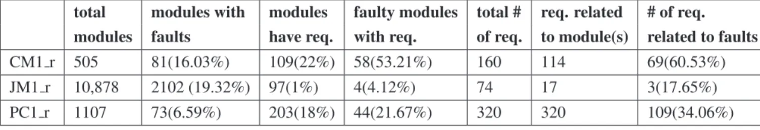
3.3 The associations between modules and requirements in CM1, JM1 and PC1. . 42

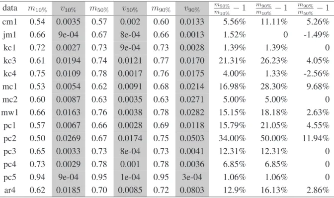
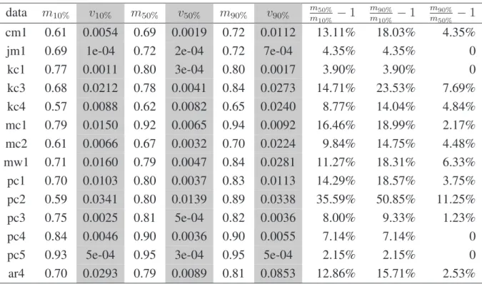
4.1 Median(m) and variance(v) of 10%, 50%, and 90% training subset models from designmetrics, measured byAUC . . . 59

4.2 Median(m) and variance(v) for models trained from 10%, 50%, and 90% of modules usingcodemetrics, measured byAUC. . . 64

4.3 Median(m) and variance(v) of models built from 10%, 50%, and 90% of module usingallmetrics, measured byAUC . . . 66

4.4 Median and variance of AUC ondesignmetrics of using50%data as the train-ing subset . . . 78

(9)

subset . . . 79

4.6 Median and variance of AUC on allmetrics of using 50%data as the training subset . . . 80

5.1 Probability cost of interested and significant ranges. . . 97

5.2 Comparison of the “best” vs. the “worst” performance classifiers. . . 100

5.3 Comparison the similarity of three different distance methods. . . 103

5.4 Priority distribution of five projects. . . 103

5.5 Probability cost of interested and significant ranges of MC1 and KC3. . . 105

5.6 Comparison of the “best” vs. the “worst” performance classifiers on MC1 and KC3. . . 105

5.7 Priority ranges and significant differences for five projects. . . 106

5.8 Performance thresholds for three priorities in KC3, PC1, and PC4 high risk projects. . . 107

5.9 Comparison of Normalized Expected Cost (NEC) with and without module spe-cific priority . . . 110

(10)

List of Figures

2.1 A confusion matrix of prediction outcomes. . . 21

2.2 ROC analysis. . . 24

2.3 ROC curve (a) and PR curve (b) of models built from PC5 module metrics . . . 25

2.4 Boxplots of PC5 data set . . . 27

2.5 An example of Demsar’s significance diagrams. . . 30

2.6 The Friedman test ondesignmetrics models using AUC for performance eval-uation. . . 31

3.1 An entity-relationship diagram relates project requirements to modules and mod-ules to faults . . . 40

3.2 CM1 r prediction using requirements metrics only. . . 43

3.3 JM1 r prediction using requirements metrics only. . . 44

3.4 PC1 r prediction using requirements metrics only. . . 45

3.5 CM1 r using module metrics. . . 46

3.6 JM1 r using module metrics. . . 47

3.7 PC1 r using module metrics. . . 48

(11)

3.9 PC1 RM model uses requirements and module metrics. . . 50

3.10 ROC curves for CM1 project. . . 51

3.11 ROC curves for JM1 project. . . 51

3.12 ROC curves for PC1 project. . . 52

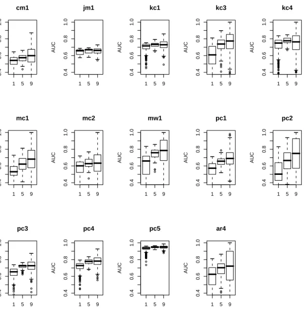
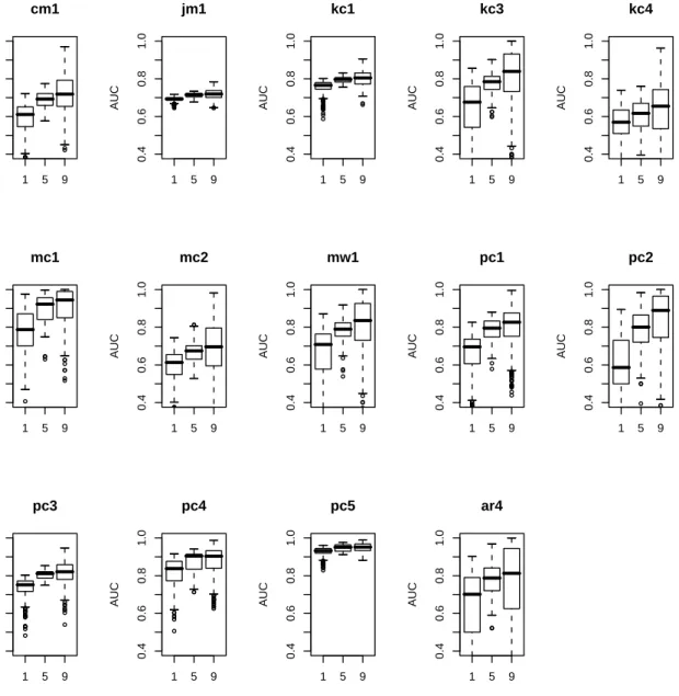
4.1 Boxplot diagrams of using 10%, 50%, and 90% data as training subset on designmetrics, measured by AUC. In x-axis, “1” stands for 10%; “5” stands for 50%; “9” stands for 90%. . . 61

4.2 The Friedman test oncodemetrics models evaluated using AUC. . . 62

4.3 Boxplot diagrams of fault prediction models built from 10%, 50%, and 90% of data usingcodemetrics, measured byAUC. In x-axis, “1” stands for 10%; “5” stands for 50%; “9” stands for 90%. . . 63

4.4 The Friedman test onallmetrics using AUC. . . 65

4.5 Box-plot diagrams of fault prediction models built from 10%, 50%, and 90% of data usingall metrics, measured byAUC. In x-axis, “1” stands for 10%; “5” stands for 50%; “9” stands for 90%. . . 67

4.6 Boxplots comparisons of the performance of models built fromdesign(d),code(c), andall(a) metrics using10%data as training subset. . . 69

4.7 Statistical performance ranks ofdesign, code, andallmodels built using 10% data for training. . . 70

4.8 Boxplots comparison of the performance ofall(a),code(c), anddesign(d) met-rics using50%of data for training. . . 73

4.9 Statistical performance ranks ofdesign, code, andallmodels built using 50% of data for training. . . 74

(12)

and three metric groups. Label “a 10” (or “d 50”), for example, stands forall

(design) metrics and 10%(50%) training subset. The reported results reflect

performance ranks over all 14 data sets. . . 77

5.1 Typical regions in cost curve. . . 88

5.2 A cost curve of logistic classifier on KC4 project data. . . 88

5.3 Cost curve of 5 classifier on KC4. . . 90

5.4 (a) A ROC curve (b) Corresponding cost curve of MC2. . . 91

5.5 The 95% cost curve confidence interval comparing IB1 and j48 on PC1 dataset. 93 5.6 Cost curves of projects. . . 96

5.7 Cost curves of MC1 and KC3 projects. . . 104

5.8 Cost curves with lowest misclassification costs for KC3, PC1, and PC4. . . 108

(13)

Chapter 1 Introduction

Significant research has been conducted to study the detection of software modules which are likely to contain faults. The fault-proneness information not only points to the need for in-creased quality monitoring during the development but also provides important advice to assign verification and validation activities. A study has shown that software companies spend 50 to 80 percent of their software development effort on testing [58]. The identification of fault-prone modules might have a significant cost-saving impact on software quality assurance.

The earlier a fault is identified, the cheaper it is to correct it. Boehm and Papaccio advise that to fix a fault early in the lifecycle, it is cheaper by a factor of 50−200 [12]. A panel of IEEE Metrics in 2002 found that fixing a severe software problem after delivery is often 100 times more expensive than that of fixing it early in requirement and design phase [78]. When it comes to software fault prediction, naturally, people would wonder whether metrics from the early lifecycle, such as requirement metrics and design metrics, are effective to predict software faults or not. In this dissertation, we will investigate:

• Q1: Are requirement metrics good fault-prone predictors for fault prediction models? • Q2: Are design metrics good enough to be built into fault prediction models?

• Q3: Are code metrics good fault-prone predictors?

A wide range of software metrics have been proposed to be collected and used to predict 1

(14)

faults [31]. There are requirement metrics [38, 40, 59], design metrics [20, 68, 70, 73, 76, 80, 94], code metrics [17,33,45,62,67], and different social network metrics, for example, the developer information [85], messages about mailing list [55], and organizational structure complexity met-rics [69]. Although there are various software metmet-rics used in the prediction of fault-proneness, comparing the effectiveness of design and code metrics received limited attention. To the best of our knowledge, the paper by Zhaoet al. is unique as it compares the performance of design and code metrics in the prediction of software fault content [91]. They compared fault predic-tion models built from design metrics, code metrics, and the combinapredic-tion of design and code metrics in the context of a large real-time telecommunication system. Their design metrics are a modified version of McCabe’s cyclomatic complexity, extracted from Specification Descrip-tion Language (SDL). They used regression equaDescrip-tions to fit their three groups of metrics and

R2 _{statistic to evaluate the performance of the models. While their findings are based on the}

analysis of a single data set, we have access to more than 10 project data sets and we analyze the effect of design metrics, and code metrics such as:

• Q4: Do fault prediction models built from a combination of requirement, design, and code metrics provide better performance than models built from any metrics subset? Besides metrics, how large is a training subset needed for building a meaningful software fault prediction model? This problem is seldom investigated although various sizes of training subsets are used in literature. For example, Menzieset al. used90%data as the training subset in his work [62]. Lessmannet al. used 2

3 data as the training subset in his study [53]. Guoet al.

use 3

4 data to build the training models [33]. In Jianget al.’s work [40],80%data is used to train

fault prediction models. In this dissertation, we would like to explore the following problems: • Q5: How large does a training subset needed to be in order to build meaningful fault

prediction models?

• Q6: How large does a training subset needed to be in order to achieve statistically the best performance fault prediction models ?

When a software project evolves into its late lifecycle stages, i.e, testing phase, it is neces-sary to analyze misclassification costs of a project and even misclassification costs for module(s) in a project. The “traditional” software fault prediction models typically assume uniform mis-classification cost. In other words, these models assume that the cost implications of wrongly

(15)

predicting a faulty module as fault free is the same as the cost of predicting that a fault free mod-ule may contain faults. In actuality, the cost implications of these two types of misclassifications are seldom equal in the real world. In high risk software projects, for example, safety-related spacecraft navigation instruments, the cost of mis-predicting a faulty module may have extreme consequence according to a loss of the entire mission. Therefore, in such projects significant resources are typically available for identifying and eradicating all faults because the cost of losing a mission is much higher. On the other hand, in low risk projects which aim to occupy a new market niche, time to market pressure may imply that only a minimal number of faulty modules can be analyzed. The cost of analyzing any significant number of misclassified fault free modules is, therefore, unacceptable.

An important factor that makes the identification of faulty modules a challenge is the reality that they usually form a minority class compared to fault free modules. We want to analyze problems associated with misclassification costs:

• Q7: How can we include misclassification costs in fault prediction models? • Q8: How can we achieve the lowest misclassification cost for a given data set?

• Q9: From misclassification cost perspective, how can fault prediction models guide dif-ferent risk level projects?

• Q10: How can we evaluate individual module’s specific misclassification costs in fault prediction models?

The remainder of this dissertation is organized as follows. Chapter 2 discusses related work. First, after introducing a brief history, associated machine learning algorithms, and approaches in fault prediction models, we review the measurements used and the appropriate statistical tests applied in software fault-proneness prediction. Chapter 3 discusses fault prediction models built from requirement metrics, and the combination of requirement metrics and software module metrics (module metrics include design metrics and code metrics). Chapter 3 will address Question Q1 and partial of Q4. Chapter 4 presents our experiments and results on incremental development of software fault prediction models comparingdesign, andcodemetrics, and their combination of both of them. Chapter 4 will answer Question Q2, Q3, Q4, Q5, and Q6. Chapter 5 describes our experiments and results to evaluate misclassification costs in fault prediction models and the cost curve to address project specific economic parameters. Chapter 5 will answer Question Q7, Q8, Q9, and Q10. Chapter 6 draws conclusions and proposes possible

(16)

(17)

Chapter 2 Related Work

Software quality engineering includes different quality assurance activities in the software de-velopment process such as testing, fault prevention, fault avoidance, fault tolerance, and fault prediction. Faults may be predicted before they cause failures. Once predicted, fault-prone modules are tested more intently than fault free modules. There are many benefits of software fault prediction such as more reasonable allocation of resources by focusing on faulty modules, improving test process, and eventually having a high quality system.

Many different techniques have been investigated in fault prediction including algorithms, statistical methods, software metrics, and software projects. Until now, researchers used differ-ent algorithms such as Genetic Programming, Decision Trees, Fuzzy Logic, Neural Networks, and Case-based Reasoning for fault prediction. Various metrics including design metrics, code metrics, test metrics, historical metrics, metrics extracted from social network associated with software products are used to predict software faults. All different kinds of statistical measure-ments are used to evaluate software fault prediction models including accuracy, probability of detection, Area Under the Curve ofROC, F-Measure, andG-meansetc.

In this chapter, we will first introduce software fault prediction models including a brief history. Second, we will present different approaches in fault prediction models. Third, we will review various metrics used in fault prediction models. Fourth, different kinds of measurements in fault prediction models are presented. Fifth, we will briefly review the research works

(18)

ducted using MDP data sets. Finally, we will discuss what has been achieved by the current state-of-the-art techniques in fault prediction, and we also point out what needs to be done in the future.

2.1 Fault Prediction Modeling

The problem of predicting the quality of a software product before it is used is challenging. Many research efforts and different kinds of methods and models have been investigated. Fault prediction allows the tester to manipulate their resources more effectively and efficiently, which would potentially result in higher quality products and lower costs.

To the best knowledge of the author, the earliest fault prediction models have been built by Akiyama in 1971 [4]. In his study, Akiyama used four regression models to fit some simple metrics, i.e, lines of code (LOC) to estimate the total number of faults in a system at Fujitsu, Japan. Interestingly, fault prediction models based on regression models are still common and useful in the software engineering literature. Another early study has been conducted by Fer-dinand [32] in 1974. FerFer-dinand proposed that the expected number of faults increases with the number of code segments.

Milestones were established by Halstead in 1975 [34] and McCabe in 1976 [60]. Halstead proposed a set of code size metrics, well known as Halstead complexity metrics in the software engineering community, to measure source codes. Halstead provided a solution to the most fundamental question in software “How big is a program (a project)?”. Since then, Halstead metrics are not only used as a measurement for developing effort, testing effort, but also are used as a set of metrics to predict software faults. McCabe proposed another important set of metrics, referred to as McCabe’s cyclomatic complexity [60]. McCabe’s metrics represent the structure of software product by measuring the software product data-flow graphs and control-flow graphs (i.e, the number of decision points, the number of links, the number of nodes, the nesting depth). Nowadays, these sets of metrics are still the primary quantitative measures in use, and they are the foundation of software engineering. After the publication of Halstead and McCabe metrics, many software fault prediction models have utilized them [7,10,11,35,62,77]. With the appearance of Object-Oriented (OO) programming languages, another important

(19)

OO metrics, referred to as CK-metrics [20], were proposed by Chidamber and Kemerer in 1994. CK metrics are proved to be effective predictors for software faults [68,80]. Halstead, McCabe, and CK metrics are all originally defined on source codes. Currently, other kinds of metrics are studied: for example, requirement metrics [40], design metrics [20], code churn [66], the historical data [74], the number of developers [85], and software product’s social networks [69]. With the development of machine learning algorithms, such as decision trees [45], neural networks [46], and genetic algorithms [8] etc., software fault prediction models advanced at a faster pace.

2.1.1 Machine Learning

Machine learning is a process in which a machine (computer) improves its performance based on “rule” (pattern) learning from previous behaviors (data). There are two essential steps involved in machine learning. First, learning knowledge from existing data; secondly, predict-ing (suggestpredict-ing) what to do in the future (on new data). Machine learnpredict-ing is successfully used in many different fields, such as medical diagnosis, bioinformatics, biometrics, credit card fraud, stock market, and software engineering. On the other hand, machine learning is also a multi-disciplinary science used by many different sciences, including statistics, artificial intelligence, information theory, computer science, control theory, biology, and other fields.

Major algorithms used in machine learning are decision trees, neural network, concept learning, genetic algorithm, reinforcement learning, and algorithms derived from them. All these algorithms have proved to be useful in the prediction of software faults. In this disserta-tion, we mainly use five different machine learning algorithms which will be introduced later: Naive Bayes, random forest, logistic regression, bagging, and boosting.

Naive Bayes

Naive Bayes is a classifier developed from the Bayes rule of conditional probability. In this dissertation, we are interested in whether a module contains a fault or not. Hence, we only consider binary classification for a module: faulty or fault-free (non-faulty). Let capital L

(20)

denoted the final class (Lis faulty or non-faulty in our case). We use a set of metrics M = (M1, M2, ..., Mn) with n number of attributes (features, or variables) to predict the final classes L.

LetP(L)denote the prior probability of a module in classLgiven a training subset data. Let

P(M)denote the prior probability that the given training data is observed. Noted that,P(M)is constant and will be eliminated in the final calculation step. LetP(L|M)denote the probability of a new module is in class Lin the condition of the training data. P(L|M)is also called the posterior probability which reflects the confidence of final class after the training data is applied.

P(L|M)is what we are interested. LetP(Mi|L)denote the probability ofMimetric (attribute)

in classLfor a given training subset. Thus, Bayes theorem is:

P(L|M) = P(L)

Q_n

i=1P(Mi|L)

P(M) (2.1)

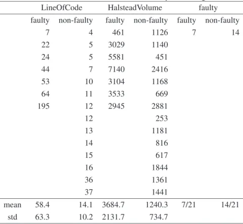
For example, we have a training subset shown as Table 2.1 which has 7 faulty modules and 14 fault-free modules. This training subset has two metrics,Lineof CodeandHalsteadV olume. The last row in Table 2.1 shows a new module with 40Lineof CodeandHalsteadV olumeof

2555. Which class will the new module be classified into given the training subset?

First, we calculate mean, standard deviation, and the number of faulty and non-faulty mod-ules of the given training subset, summarized in Table 2.2.

Because we deal with numeric attributes, the probability will be calculated according to the probability density function. The probability density function for a normal distribution with meanµand standard deviationσis given by the expression:

f(x) = √1

2πσe

(x−µ)2

2σ2 (2.2)

For the new module, withLineOfCode = 40 andHalsteadVolume=2555, the probabilities of it belonging to faulty class and non-faulty class are calculated as follows.

f(LineOf Code= 40|f aulty) = _√ 1

2π∗63.3e

(x−58.4)2

2∗63.32 = 0.00657

f(LineOf Code= 40|nonf aulty) = _√ 1

2π∗10.2e

(x−14.1)2

2∗10.22 = 0.983

f(HalsteadV olume= 2555|f aulty) = _√ 1

2π∗2131.7e

(x−3684.7)2

2∗2131.72 = 0.000215

f(HalsteadV olume= 2555|nonf aulty) = _√ 1

2π∗734.7e

(x−1240.3)2

(21)

Table 2.1. An example of training subset

LineOfCode HalsteadVolume faulty

4 1126 FALSE 10 1140 FALSE 5 451 FALSE 16 2416 FALSE 11 1168 FALSE 7 669 FALSE 37 2881 FALSE 36 253 FALSE 12 1181 FALSE 13 816 FALSE 15 617 FALSE 12 1844 FALSE 14 1361 FALSE 5 1441 FALSE 7 461 TRUE 24 3029 TRUE 64 5581 TRUE 195 7140 TRUE 44 3104 TRUE 53 3533 TRUE 22 2945 TRUE new module 40 2555 ?

(22)

Table 2.2. Summarized statistics of the example training subset.

LineOfCode HalsteadVolume faulty faulty non-faulty faulty non-faulty faulty non-faulty

7 4 461 1126 7 14 22 5 3029 1140 24 5 5581 451 44 7 7140 2416 53 10 3104 1168 64 11 3533 669 195 12 2945 2881 12 253 13 1181 14 816 15 617 16 1844 36 1361 37 1441 mean 58.4 14.1 3684.7 1240.3 7/21 14/21 std 63.3 10.2 2131.7 734.7

(23)

Using these probabilities to predict the new module, we have:

Likelihood of faulty =P(f aulty)P(LineOf Code=40|f aulty)∗P_P(₍HalsteadV olumne_M₎ =2555|f aulty)

= 7

21 ∗ 0.00657P∗(M0.000215) = 4.P72(eM−)07

Likelihood of non-faulty =P(nonf aulty)P(LineOf Code=40|nonf aulty)∗P_P(₍HalsteadV olumne_M₎ =2555|nonf aulty)

= 14

21 ∗ 0.983P∗(0M.00269) = 0.001763702P(M)

Which leads to the probabilities of the new module as follows: Probability of faulty == 4.72e−07

4.72e−07+0.001763702 = 0.00027

Probability of non-faulty = 0.001763702

4.72e−07+0.001763702 = 0.99973

Thus, using the Naive Bayes classifier, the new module with LineOfCode=40 and Halstead-Volume=2555 will be classified as fault free module.

NaiveBayes have been used extensively in fault-proneness prediction [39, 40, 62].

Logistic Regression

Regression analysis is used for explaining or modeling the relationship between a predicted variable (response variable, i.e, classL in our case) and one or more predictors, metrics M = (M1, M2, ..., Mn) (n ≥ 1). When n = 1, it is called simple regression; when n ≥ 1, it is

called multiple regression (or multivariate regression). In our case, we have multiple predictors (multiple metrics), hence, our regression is multiple regression. When the predicted (response) variable is numeric, linear regression and logistic regression can be used. However, when the predicted variable is binomial (binary classification as fault or fault-free, denoted as 1 or 0), logistic regression will be adapted.

Referring back to the previous notation, P(L|M)denotes the probability of a module in class L(faulty or non-faulty) given a set of metrics in a training subset. Then P(f aulty|M)

would be the probability of a faulty module given a set of metrics. Because this is binary classification, then 1− P(f aulty|M) would be the probability of a fault-free module for a

(24)

given set of metrics. AbbreviatedP(f aulty|M)as P, Logistic regression is defined as:

logit(P) =log P

1−P, with, P =

1

1 +e−β0−β1M1−β2M2−...−βnMn (2.3) whereβ0 is the regression intercept andβi is regression coefficient for MetricMi (i ≥ 1).

Note that, in Equation 2.3, the interactions between variables are not considered. Using the training data in Table 2.1 as an example, we have β0 = 3.9455, β1 = −0.0277, and β2 =

−0.0012. The final model for the given training data in Table 2.1 is:

P = 1

1 +e−3.9455+0.0277∗LineOf Code+0.0012∗HalsteadV olume (2.4)

Taking the metrics of the new module into Equation 2.4, we have P = 0.44, that is, the probability of this new module being faulty is44%. Then the probability of it being fault-free

is1−44% = 56%. Using 50%as the classification boundary, the new module is classified as

fault-free.

Logistic regression analysis is widely used to predict fault-proneness modules in software engineering [66, 67, 69]. The advantage of regression analysis is its flexibility of combining it to other algorithms, for example, a classification tree, to form a regression tree algorithm.

Bootstrap

Three ensemble classifiers, the random forest, bagging, and boosting all utilize the bootstrap method. Therefore, before we introduce them, we need to introduce the bootstrap method. The bootstrap method is based on sampling with replacement to form a training subset. The bootstrap method works as follows. Given a data set with n modules, bootstrap samples n

modules from the original data set with replacement to act as training data. The sampled n

modules will be repeated and there must be some modules in the original data set that are not picked into the new sampled data. Those unpicked modules will be left as testing data.

Each module in a data has the probability of 1

nbeing picked into a bootstrapped data. Thus,

the probability of not being picked is 1− 1

n. After n times of picking, the probability of a

(25)

(1− 1

n)n≈e−1 = 0.368

witheas natural logarithms (≈ 2.7183). Therefore, for each bootstrap, there are36.8%of data that are not picked and is used as testing data. The training data, although it hasninstances, only contains63.2%of the original data. Thus, the bootstrap method is often called0.632bootstrap. The bootstrap method usually is repeated several times, and then the result will be determined by majority vote (in our case) or by average when the prediction outcome is numeric.

Random Forest

Random Forest is a decision tree-based ensemble classifier which is designed by Breiman [14]. As implied from its name, it builds an ensemble, i.e., the forest of classification trees using the following strategy:

1. Each decision tree has been built from a different bootstrap sample.

2. At each node, a subset of variables are randomly selected to split the node. 3. Each tree is grown to the largest extent possible without pruning.

4. When all trees (at least 500 as recommended by its designer) in the forest are built, test instances are fitted into all the trees and a voting process takes place.

5. The forest selects the classification with the most votes as the prediction of new instances.

Random forest as a machine learning classifier provides many advantages [14]. It also auto-matically generates the importance of each attribute in the process of classification. Hence, it is a good algorithm to perform Feature Subset Selection. In empirical studies, Random forest usually is one of the best learners in fault-proneness prediction [33, 39, 40].

Bagging

(26)

1. For a training subset withnnumber of samples, it resamplesnnumber of samples from this training subset with replacement using the bootstrapping method.

2. Building a model using a base classifier (default as REPtree in Weka)

3. For a testing sample, the model predicts a class (faulty or fault-free, in our case). And the predicted class is stored for later usage.

4. Repeat the above steps for multiple times (default value is 10 in Weka) 5. Using the most predicted class for a testing sample.

We can see that bagging relies on an ensemble of different based models. Bagging shares a lot of similarity with random forest,

• The training data is resampled from the original data set with replacement.

• It is an ensemble of base classifiers. Bagging can have any kinds of basic algorithm, while random forest is only based on tree algorithm.

• The final prediction is voted by majority.

If bagging uses the same base classifier as the random forest, these two algorithms are essential the same. According to Witten and Frank [87], bagging typically performs better than single method models and almost never significantly worse. And it has good performance in our experiments [39, 40] too.

Boosting

The boosting algorithm combines multiple models by explicitly seeking models that comple-ment one another [87]. The boosting as an ensemble algorithms has many similarities with bagging (or random forest ):

• first of all, it is an ensemble of multiple based models.

• the ensemble of models are built on resampling with replacement from training subset. • the prediction outcome is determined by voting.

(27)

But there are differences between bagging and boosting.

• After the learning process is begun, the base models for boosting can be built on different algorithms, while the base algorithm of bagging never changed once it is determined. • The base classifier for boosting is iterative, that is, each new model is influenced by

the performance of those built previously, while bagging builds each new base classifier separately.

• The final voting outcome is voted differently: boosting weights each model’s prediction according to its performance while bagging treats every vote equally. By weighting in-stances, the boosting hopes to concentrate on a particular set of inin-stances, for example, those with high weight.

The random forest, bagging and boosting ensemble learners have been developed in the past decade and have proved to have astonishingly good performance in data mining [87]. In our experiments of fault prediction modeling, they demonstrate superior performance than other learners [39, 40].

2.2 Different Approaches for Fault Prediction Models

A project manager needs to make sure a project met its timetable and budget plan without loss of quality. In order to help project managers to make a decision, fault prediction models play an important role to allocate software quality assurance resources. Existing research in software fault-prone models focus on predicting faults from these two perspectives:

• The number of faults or fault density: This technique predicts the number of faults (or fault density) in a module or a component. Project managers can use these predictions to determine the process of software timetable and V&V resources allocation. These models typically use data from historical versions (or pre-release parts) and predict the faults in the new version (or the new developed parts). For example, the fault data from historical releases can be used to predict faults in updated releases [36, 51, 74].

• Classification: Classification predicts which modules (components) contain faults and which modules don’t. The goal of this kind of prediction distinguishes fault free subsys-tems from faulty subsyssubsys-tems. This allows project managers to focus resources to fix faulty

(28)

subsystems. Many software fault prediction models are this type of study [7,53,62,63,77] including this dissertation.

2.2.1 Supervised Learning

There are two methods to classify fault-prone modules from fault free modules: supervised learning and unsupervised learning. Both of them are used in different situations. When a new system without any previous release is built, for the new developed subsystems (modules, com-ponents, or classes), in order to predict fault-prone subsystems, unsupervised learning needs to be adopted. After some subsystems are tested and put into function, these pre-release sub-systems can be used as training data to build software fault prediction models to predict new subsystems. This is the time when supervised learning can be used. The difference between supervised and unsupervised learning is the status of training data’s class, if it is unknown, then the learning is unsupervised, otherwise, the learning is supervised learning.

A learning is called supervised because, the method operates under supervision provided with the actual outcome for each of the training examples. Supervised learning requires known fault measurement data (i.e, the number of faults, fault density, or fault-prone or not) for training data. Usually, Fault measurement data from previous versions [74], pre-release [65], or similar project [48] can act as training data to predict new projects (subsystems).

Most research reported in fault prediction is supervised learning including experiments in this dissertation. The learning result of supervised is easier to judge than unsupervised learn-ing. This probably helps to explain why there are abundant reports on supervised learning in the literature and there are few reports on unsupervised learning. Like most research conducted in fault prediction, a data with all known classes is divided into training data and testing data: the classes for training data are provided to a machine algorithm, the testing data acts as the validation set and is used to judge the training models. The success rate on test data gives an objective measure of how well the machine learning algorithm performs. When this process is repeated multiple times with randomized divided training and testing sets, it is the standard data mining practice, called cross-validation. Like other research in data mining, randomiza-tion, cross-validarandomiza-tion, and bootstrapping are often the standard statistical procedures for fault prediction in software engineering.

(29)

2.2.2 Unsupervised Learning

Sometimes we may not have fault data or we may have very little modules having previous fault data. For example, if a new project is developing or previous fault data is not collected, supervised learning approaches do not work because we do not have labeled training data. Therefore, unsupervised learning approaches such as clustering methods may be applied. How-ever, research for this approach is seldom reported. As far as the author is aware, Zhong et al.[92, 93] are the first group who investigate this in fault prediction. They use Neural-Gas and K-means clustering to class software modules into several groups, with the help of human ex-perts to identify fault-prone or not fault-prone to each groups. Their results indicate promising potentials for this unsupervised learning method. Interestingly, their two data sets are JM1 and KC2 from NASA MDP repository and they only use 13 metrics among 39 (or 40) total metrics.

2.3 Metrics Used in Software Fault Prediction Models

In this section, we will introduce various metrics which have been used to predict software faults. These metrics include requirement metrics, design metrics, code metrics, and other different kinds of metrics.

Requirement metrics have been used to predict fault prone software modules [38, 40, 59]. Malaiya et al. examined the relationship between requirement changes and fault density and found a positive correlation [59]. Javed et al. [38] investigate the impact of requirement insta-bility on software faults. In 4 industrial e-commerce projects and 30 releases they found: (1) a significant relationship between pre/post release change requests and overall software faults; (2) insufficient and inadequate client communication during system design phase cause require-ments changes and, consequently, software faults.

One of the earliest studies of design metrics in fault prediction models was conducted by Ohlsson and Alberg [73]. They predicted fault-prone modules prior to coding in a Telephone Switches system of 130 modules at Ericsson Telecom AB. Their design metrics are derived from graphs where functions and subroutines in a module are represented by one or more graphs. These graphs, called Formal Description Language (FDL) graphs, offer a set of direct and

(30)

indi-rect metrics based on the measures of complexity. Examples of diindi-rect metrics are the number of branches, the number of graphs in modules, the number of possible connections in a graph, and the number of paths from input to the output signals etc. Indirect metrics are the metrics calculated from the direct metrics such as McCabe cyclomatic complexity.

The suite of object oriented (OO) metrics, referred as CK metrics, has been first proposed by Chidamber and Kemerer [20]. They proposed six CK design metrics including Weight Method Per Class (WMC), Number of Children (NOC), Depth of Inheritance Tree (DIT), Coupling Between Object class (CBO), Response For a Class (RFC), and Lack of Cohesion in Methods (LCOM). Basili et al. [9] were among the first to validate these CK metrics using 8 C++ sys-tems developed by students. They demonstrated the benefits of CK metrics over code metrics. In 1998, Chidamber, Darcy and Kemerer explored the relationship between the CK metrics and productivity, rework effort or design effort [19]. They show that CK metrics have better ex-planatory power than traditional code metrics. Predicting fault-prone software modules using metrics from design phase has recently received increased attention [62, 74, 76, 88]. In these studies, metrics are either extracted from design documents or, like in our work, by mining the source code using the reverse engineering techniques. Subramanyam and Krishnan predict faults from three design metrics: Weight Method Per Class (WMC), Coupling Between Object Class (CBO), and Depth of Inheritance Tree (DIT) [80]. The system they study is a large B2C e-commerce application suite developed using C++ and Java. They showed that these design metrics are significantly related to faults and that faults are strongly related to the language used. Nagappan, Ball and Zeller [68] predict component failures using OO metrics in five Mi-crosoft software systems. Their results show that these metrics are suitable to predict software faults. They also show that the predictors are project specific, the suggestion also mentioned by Menzies et al. [62].

Recovering design from source code has been a hot topic in software reverse engineer-ing [5, 6, 16]. Systa [81] recovered UML diagrams from source code usengineer-ing static and dynamic code analysis. Tonella and Potrich [82] were able to extract sequence diagrams from source code. Briand et al. demonstrated sequence diagrams, conditions and data flow can be reverse engineered from Java code through transformation techniques [15].

Recently, Schroter, Zimmermann, and Zeller [76] applied reverse engineering to recover design metrics from source code. They used 52 ECLIPSE plug-ins and found usage

(31)

relation-ships between these metrics and past failures. The relationship they investigate is the usage of import statements within a single release. The past failure data represents the number of fail-ures for a single release. They collected the data from version archives (CVS) and bug tracking systems (BUGZILLA). They built predictive models using the set of imported classes of each file as independent variables to predict the number of failures of the file. The average prediction accuracy of the top5% is approximately 90%. Zimmermann, Premraj and Zeller [94] further investigate ECLIPSE open source, extract object oriented metrics along with static code com-plexity metrics and point out their effectiveness to predict fault-proneness. Their data set is now posted in the PROMISE [13] repository. Neuhaus, Zimmermann, Holler and Zeller ex-amine Mozilla code to extract the relationship of imports and function calls to predict software components vulnerabilities [70].

Besides requirement metrics, design metrics, and code metrics, various other measures have been used to predict fault prone software modules. Historical project characteristic, devel-oper information and social networks have all been reported as effective predictors. Ostrand, Weyuker, and Bell [74] predict the files most likely to contain the largest numbers of faults in the next release using modification history from previous release and the code in the current release. Illes-Seifert and Paech investigate the relationship between software history character-istics and the number of faults [36]. After analyzing 9 open source Java projects, they conclude that some history characteristics, such as the number of changes and the number of distinct authors performing changes to a file, highly correlate with faults. Code churn, defined as the amount of code change taking place within a software unit [66], also called cached history [51], was also reported as an effective predictor of faults.

The role of developer social networks is currently receiving significant attention. Weyuker, Ostrand, and Bell [85] found that the addition of developer information improves the accuracy of fault prediction models. Li et al. analyzed 139 metrics collected from software product, de-velopment, deployment, usage, software and hardware configurations in OpenBSD [55]. They found that the number of messages to the technical discussion mailing list during the devel-opment period is the best predictor of the number of field faults. Nagappan et al. [69] collect 8 organizational structure complexity metrics which relate code binary to the organizational social networks, i.e, the number of engineers, the number of ex-engineers, edit frequency of source code, and organization intersection factors to predict failure-proneness. They compare

(32)

this model to models which use five groups of traditional metrics (code churn, code complexity, code coverage, dependency, and pre-release bugs). The use of organizational structure com-plexity metrics appears to hold a significant promise for fault prediction.

2.4 Model Evaluation Techniques

Many statistical techniques have been proposed to predict fault-proneness of program mod-ules in software engineering. Choosing the “best” candidate among many available models involves performance assessment and detailed comparison. But these comparisons are not sim-ple due to the applicability of varying performance measures. Classifying a software module as fault-prone implies the application of some verification activities, thus adding to the develop-ment cost. Misclassifying a module as fault free carries the risk of system failure, also associated with cost implications. Methodologies for precise evaluation of fault prediction models should be at the core of empirical software engineering research, but have attracted sporadic attention. In this chapter we overview model evaluation techniques. In addition to many techniques that have been used in software engineering studies before, we introduce and discuss the merits of cost curves.

2.4.1 Methodology for 2-class Classification

We are interested in the identification of fault-proneness information of software, that is, which parts contain faults. Requirement metrics, design metrics, code metrics, and the fusion of these metrics serve as predictors. And the predicted variable is whether a fault is detected in the given software units. Throughout the measurement in this dissertation, the confusion matrix of 2-class classification serves as the foundation of measurement. All kinds of mea-surement used in this disseartation are derived from the confusion matrix. Figure 2.1 describes the confusion matrix of prediction outcomes. The confusion matrix has four categories: True positives (TP) are modules correctly classified as faulty modules. False positives (FP) refer to fault-free modules incorrectly labeled as faulty modules. True negatives (TN) correspond to fault-free modules correctly classified as such. Finally, false negatives (FN) refer to faulty modules incorrectly classified as fault-free modules.

(33)

Figure 2.1. A confusion matrix of prediction outcomes. P D =recall= T P T P+F N P F = F P F P+T N acc= T P+T N T N+T P+F P+F N p=precision= T P F P+T P sp=specif icity= 1−P F = T N T N+F P G−mean 1 = √P D∗p G−mean 2 = √P D∗sp F −measure= (β_β2+1)2_∗_p₊∗p_{P D}∗P D J coef f = P D−P F

The Probability of Detection (P D), also called recall or specificity in some literature [33, 62]), is defined as the probability of the correct classification of a module that contains a fault. The Probability of False alarm (P F) is defined as the ratio of false positives to all non-faulty modules. Accuracy (acc) is widely used in all kind of data mining classifiers. It is the ratio of sum of true positive and true negative to total number of units studied, that is, the overall ratio of correctly predicted units. Thus, acc gives the overall classification performance of a classifier. However,it ignores the data distribution and cost information. Therefore, it can be a misleading criterion as faulty modules are likely to represent a minority of the modules in the dataset [57]. Precision (p) is the proportion of the predicted faulty software units that actually contain fault(s). It is shown that precision is not a suitable measurement to evaluate software quality model alone [61]. Specificity shows how well a classifier correctly identifies the non-faulty cases, that is, it is the proportion of true negatives of all non-non-faulty in a project.

Compared to overall accuracy, F-measure [54], geometric mean (G-mean) [52], and J coef-ficient (J coef f) [89] tell a more honest story about model’s performance. G−mean1 is the

(34)

square root of the product of sensitivity (PD) and precision. G−mean2is the square root of the

product ofP D and specificity. In software quality prediction, it may be critical to identify as many fault-prone modules as possible (that is, a high sensitivity or PD). If two methodologies produce the same or similar PD, we prefer the one with higher specificity. So, G-mean2 is the geometric mean of two accuracies: one for the majority class and another for the minority class. Precision tells us among all the faulty modules the model may have discovered, how many are actually faulty. BothG−mean1and F-measure integrateP Dandprecisionin a performance

index. F-measure offers more flexibility by including a weight factor β which allows us to manipulate the weight (cost) assigned to PD and precision. Parameterβ may assume any non-negative value. If we setβto 1, equal weights are given to PD and precision. The weight of PD increases as the value ofβ increases.

Youden proposed J coefficient (J coef f) to evaluate measurements in medical sciences [89]. El-Emam et al. were the first to use J coefficient to compare classification performance in software engineering [27]. The formula is J coef f = sensitivity + specif icity − 1 =

P D −1 +specif icity = P D − (1−specif icity) = P D −P F. We can see that J

coef-ficient is a combination of PD and PF. WhenJ coef f = 0, the probability of detecting a faulty module is equal to the false alarm rate. Such a classifier is not very useful. WhenJ coef f >0,

P Dis greater thanP F, a desirable classification result. Hence,J coef f = 1represents perfect classification, whileJ coef f =−1is the worst case.

Variance is a measure of statistical dispersion of a random variable, computed by averaging the squares of the deviations. When evaluating performance of a classification experiment, the smaller the variance, the more “reliable” (stable) the classifier performs. Although the impor-tance of variance in the supervised classification is known, it is seldom reported and analyzed in software fault prediction models. Assumeµstands for the mean, µ= Pxi

n , variance,s2, is calculated as follows: s2 = P (xi−µ)2 n−1 (2.5)

The standard deviation,σ, is the square root of variance, that is,σ =√s2_{. Noted that, in the}

supervised classification, many commonly used performance indices, such as,recall, precision, PF, and AUC, are all from0 to1. As a consequence, variances are all less than 1. This does not imply that variance is small. From an empirical perspective, if variance is greater than0.05,

(35)

then the classification has a larger variance [44].

2.4.2 Graphical Evaluation Methods

In this section, we present Receiver Operating Characteristic (ROC) curve, Precision and Recall (PR) curve, and Lift Chart etc. These graphs are closely related, being derived from the confusion matrix. Ling et al. discussed the relationship between ROC and lift chart [56]. In [84], Vuk and Curk establish a common mathematical framework between ROC and lift chart, and the Area Under the ROC Curve (AUC) and Area Under the Lift Chart. However, each curve reveals different aspects of classification performance, making them worth considering in software engineering projects.

ROC Curve

Many classification algorithms allow users to define and adjust a threshold parameter in order to generate an appropriate classifier. When predicting software quality a higher PD can be produced at the cost of higher PF and vice versa. The (PF, PD) pairs generated by adjusting the algorithm’s threshold form a Receiver Operating Characteristic (ROC) curve. ROC analysis is a more general way to measure a classifier’s performance than numerical indices [90]. An ROC curve provides a visual tool for examining the tradeoff between the ability of a classifier to correctly detect fault-prone modules (P Dorsensitivity) and the number of non-fault-prone modules that are incorrectly classified (PF, or1−sp).

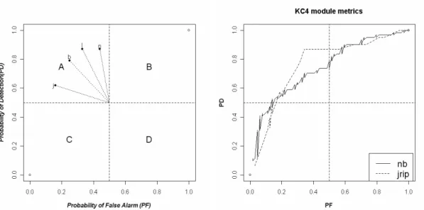
The Area Under the ROC curve, referred to as AUC, is a numeric performance evaluation measure that is directly associated with an ROC curve. It is very common to use AUC to compare the performance of different classification methods based on the same data. However, large parts of the region under the curve are typically not of interest to software engineers. For instance, the regions associated with very low probability of detection (region C in Figure 2.2(a)) or very high probability of false alarm (region B in Figure 2.2(a)) or both (region D in Figure 2.2(a)), typically indicate poor performance. With a few possible exceptions (for example safety critical systems, in which risk aversion drives the development process), only the performance points associated with acceptable P D and P F rates (region A) are likely to

(36)

have a practical value for software engineers. Therefore, in software engineering studies, the area under the curve of region A (denoted AUCa) is typically a more meaningful method to make the comparison than the standard AUC.

Figure 2.2. (a) Four possible regions represent various performance of software fault pre-diction models; (b) ROC curves from two classifiers Naive Bayes (nb) and jrip on project KC4.

The utility of this comparison method extends to classifiers which lack the flexibility of generating an ROC curve, since they typically lack the threshold parameter. Such algorithms are only capable of producing a single point in the space represented by a (P F, P D) pair. Rather than measuring distances from an arbitrary reference point, one can calculate as the dis-tance from the perfect classification point (0, 1) to the (PF, PD) pair point, defined asED[62]:

ED=pθ∗(1−P D)2_{+ (1}₋_θ₎_∗_{P F}2_,

whereθis a parameter ranging from 0 to 1, used to control weights assigned to 1-sensitivity (i.e., 1-PD) and 1-specificity (i.e., PF). The smaller the distance, i.e., the closer the point is to

(37)

the perfect classification, the better the performance of the associated classifier. This distance from perfect point (0,1) is appropriate to choose a best point from a convex hull of an ROC curve too. This method can assist software engineers in determining the “best” threshold for a classifier, given a project data and an appropriate value of parameter .

Precision-Recall curve

Precision-Recall (PR) curve presents an alternate approach to the visual comparison of classi-fiers [22]. PR curve can reveal the difference between algorithms which is not apparent from an ROC curve. In a PR curve, x-axis represents recall and y-axis is precision. Recall is yet another term for PD. (a) (b) 0.0 0.2 0.4 0.6 0.8 1.0 0.0 0.2 0.4 0.6 0.8 1.0 PC5 module metrics PF PD NB RF IBk 0.0 0.2 0.4 0.6 0.8 1.0 0.0 0.2 0.4 0.6 0.8 1.0 PC5 module metrics Recall Precision NB RF IBk (a) (b)

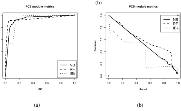
Figure 2.3. ROC curve (a) and PR curve (b) of models built from PC5 module metrics

Figure 2.3 shows an example. Looking at the ROC curves for project PC5, it is difficult to tell the difference among three classifiers: Naive Bayes (nb), Random Forest (RF), and IBk.

(38)

However, their PR curves allow us to understand the difference in their performance: Random Forest algorithm performs better than Naive Bayes and Naive Bayes has an advantage over IBk. In ROC curves, the best performance indicates high PD and low PF in the left-hand upper corner of the curve. PR curves favor classifiers which offer high PD and high Precision, i.e., the ideal performance goal lays in the right-hand upper corner. In Figure 2.3(a), the performance of the three classifiers appears to approach close to the optimal left-hand upper corner. However, the PR curve of Figure 2.3(b) indicates that there is still plenty of room for the improvement of classification performance. We do not say that PR curves are better than ROC curves. We only recommend that when ROC curves fail to reveal differences in the performance of different classification algorithms, PR curves may provide adequate distinction.

Lift Chart

In practice, every software project has a finite time and budget constraints for verification and validation. Given the fault prediction model, the question that typically arises is how to utilize available resources to achieve most effective quality improvement. Lift charts [87], known in software engineering as Alberg diagrams [47, 72–74], are another visual aid for measuring classification performance. Lift is a measurement of the effectiveness of a classifier to detect faulty modules. It calculates the ratio of correctly identified faulty modules with and without the predictive model. Lift chart is especially useful in situations when the project has limited resources to apply verification activities to, say,5% of the modules. Which model selects the

5%of the project’s modules with a largest probability that these modules contain faults? Lift chart analysis starts by ranking all the modules with respect to their chance of contain-ing fault(s). The rankcontain-ing methods can vary [47, 56, 72–74, 87]. For example, some algorithms (i.e. multiple linear regression models) may use the expected number of faults in a module. Alternatively, a classifier may output a score indicating the likelihood that the module belongs to a faulty class (i.e. Naive Bayes). An ensemble algorithm (random forest) may count the vot-ing score. Once modules are ranked, we calculate the number of faulty modules in the specific rank (from 0to 100%). In the lift chart, the x-axis represents the percentage of the modules considered, and the y-axis indicates the corresponding detection rate within this sample. The lift chart consists of a baseline and a lift curve. The lift curve shows the detection probability

(39)

resulting from the use of the predictive model, while the baseline indicates the proportion of faulty modules in the data set. The greater the area between the lift curve and the baseline is, the better the performance of the classifier is.

Boxplot Diagrams

A boxplot, also known as a box and whisker diagram, graphically depicts numerical data dis-tributions using five first order statistics: the smallest observation, lower quartile (Q1), median, upper quartile (Q3), and the largest observation. The box is constructed based on the interquar-tile range (IQR) from Q1 to Q3. The line inside the box depicts the median which follows the central tendency. The whiskers indicate the smallest observation and the largest observation. Figure 2.4 shows an example boxplot of the best learners on the three groups of metrics on PC5 data set.

all:rf code:bag design:bag

0.960

0.965

0.970

0.975

Comparison of the best learners in PC5

Area Under the Curve (AUC)

(40)

2.4.3 Statistical Comparisons of Classification Models

Drawing sound decisions from performance comparison of different classification algo-rithms is not simple. Statistical inference is often required. The purpose of performance com-parison is to select the best model(s) out of several candidates. Suppose there are kmodels to compare. The statistical hypotheses are:

H0: There is no difference in the performance among k classifiers.

vs.

Hα: At least two classifiers have significantly different performance.

When more than two classifiers are under comparison, a multiple test procedure may be appropriate. If the null hypothesis of equivalent performance among k classifiers is rejected, we need to know which differences cause the rejection. In order to better understand why H0 is rejected we need to conduct pairwise comparison, that is, compare the performance difference between pairs of classifiers. We will then have the follow up statistical hypotheses for compar-ison between two classifiers:

H0: There is no difference in the performance between the two classifiers.

vs.

Hα: There is a significant difference in the performance of the two classifiers.

The most popular method used to evaluate a classifier on a data set is10by10ways cross-validation (10x10 CV). The10x10CV results in10values of the performance index of interest (AUC, F-measure, or any other). These 10 values are likely similar to each other, given that they come from the same population. But, given the 10 values it is difficult to establish whether they follow the normal distribution (i.e., indicate that they obey the central limit theorem). Therefore, using parametric statistical methods, which assume the normally distributed population, may not be justified. A prudent approach calls for the use of nonparametric methods. The loss of efficiency caused by using nonparametric tests is typically marginal [21, 79].

Demsar [23] overviewed theoretical work on statistical tests for classifier comparison. He recommended the Wilcoxon signed rank test for the comparison of two classifiers and the

(41)

Fried-man test with the corresponding post-hoc tests, the Nemenyi test, when the comparison includes more than two classifiers. The Wilcoxon signed rank test and the Friedman’s test are nonpara-metric counterparts for paired t test and analysis of variance (ANOVA) paranonpara-metric methods, respectively. Demsar advocates these tests largely due to the fact that nonparametric proce-dures make less stringent demands on the data. However, two issues need attention. First, nonparametric tests do not utilize all the information available. The actual data values (in our case performance indices such asAUC) are not used in the test procedure. Instead, the signs or ranks of the observations are used. Therefore, parametric procedures will be more power-ful then their nonparametric counterparts, when justifiably used. The second point is that the signed rank tests are constructed for the null hypothesis that the difference of the performance measure is symmetrically distributed. For non-symmetric distributions, this test can lead to a wrong conclusion.

Demsar used a significance diagram to represent test result, called Demsar’s significance

diagram. An example is shown in Figure 2.5. The figure shows the result of Demsar’s

proce-dure oncm1 designmetrics, comparing models from 5 different training sizes, measured by

AUC. The statistical hypotheses are:

H0:The size of the model’s training set has no influence on model performance among 10 dif-ferent runs in cm1 design metrics.

vs.

Hα: Some (at least two) models developed using different training subset sizes result in

signifi-cantly different performance among 10 different runs in cm1 design metrics.

Let’s look at Figure 2.5. The numbers in the scale represent the average rank; the higher the rank, the worse the performance of a training size. Therefore, from the worst towards the best, the order of models is from 10%to90%. In Figure 2.5, the critical difference (CD) is 2.728. When the difference between two average ranks (or two models) is smaller than the value of

CD, the difference in their performance is not significant, as connected by a bold straight line. Figure 2.5 indicates that our fault prediction models form two performance clusters: one is10%,

25%,50%, and75%; the other is 25%, 50%, 75%, and 90%.

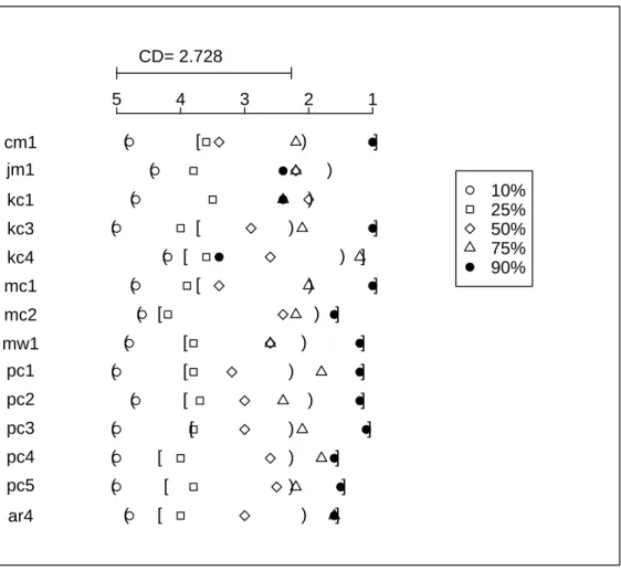
With more than one data set, we used a modified version of Demsar’s significance diagrams. Let’s compare Demsar’s significance diagram shown in Figure 2.5 to the first item (the same

(42)

5 4 3 2 1 10% 25% 50% 75% 90%

CD = 2.728

Figure 2.5. An example of Demsar’s significance diagrams.

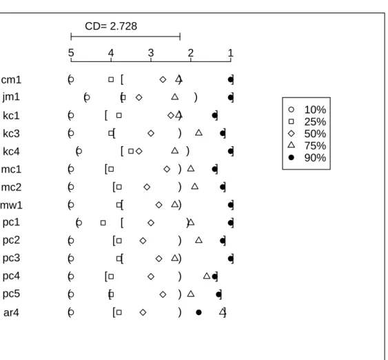
test on cm1 data) in Figure 2.6. The rank is still represented on a horizontal scale from 1 to 5: the higher the rank, the worse the performance of a training size. CD still represents the critical difference value for this statistical test. However, two straight lines are replaced with two bracket pairs: round and square bracket. The models inside each bracket do not have any statistical difference. The round bracket forms the worst performance models while the best performance models are enclosed inside the square bracket. In this way, Figure 2.6 is able to show the test result of14data sets.

2.5 MDP Data Sets and Prior Experiments

The 16 data sets used in this dissertation come from the NASA MDP repository [2] and PROMISE (3 data sets) [13] shown in Table 2.3. Metrics Data Program (MDP) is a software metrics repository provided by NASAIV&V and is available to general users through website http://mdp.ivv.nasa.gov/. MDP data stores and organizes the software product metrics data and associated error data at the module (functional/method) level. Currently, there are 13 projects data available. All MDP data are also available from PROMISE [13] public repository. Public fault data repository provide a possible platform for comparison of different approaches, dif-ferent measurements, and difdif-ferent research groups worldwide. With the availability of public fault data sets, fault prediction are able to be investigated in a repeatable, or improvable, or even refutable way.

(43)

CD= 2.728 1 2 3 4 5 cm1 ( [ ) ] jm1 ( ) kc1 ( ) kc3 ( [ ) ] kc4 ( [ ) ] mc1 ( [ ) ] mc2 ( [ ) ] mw1 ( [ ) ] pc1 ( [ ) ] pc2 ( [ ) ] pc3 ( [ ) ] pc4 ( [ ) ] pc5 ( [ ) ] ar4 ( [ ) ] 10% 25% 50% 75% 90%

Figure 2.6. The Friedman test ondesignmetrics models using AUC for performance evalu-ation.

(44)

Table 2.3. Datasets used in this dissertation

Data mod.# %faulty project description lang. source

JM1 10,878 19.3% Real time predictive ground system C MDP MC1 9466 0.64% Combustion experiment of a space shuttle (C)C++ MDP PC2 5589 0.42% Dynamic simulator for attitude control systems C MDP PC5 17,186 3.00% Safety enhancement system C++ MDP PC1 1109 6.59% Flight software from an earth orbiting satellite C MDP PC3 1563 10.43% Flight software for earth orbiting satellite C MDP PC4 1458 12.24% Flight software for earth orbiting satellite C MDP

CM1 505 16.04% Spacecraft instrument C MDP

MW1 403 6.7% Zero gravity experiment related to combustion C MDP KC1 2109 13.9% Storage management for ground data C++ MDP KC3 458 6.3% Storage management for ground data Java MDP KC4 125 48% Ground-based subscription server Perl MDP MC2 161 32.30% Video guidance system C++ MDP

ar3 63 12.70% Refrigerator C PROMISE

ar4 107 18.69% Washing machine C PROMISE