HAL Id: lirmm-01056150
https://hal-lirmm.ccsd.cnrs.fr/lirmm-01056150
Submitted on 16 May 2020
HAL
is a multi-disciplinary open access
archive for the deposit and dissemination of
sci-entific research documents, whether they are
pub-lished or not. The documents may come from
teaching and research institutions in France or
abroad, or from public or private research centers.
L’archive ouverte pluridisciplinaire
HAL
, est
destinée au dépôt et à la diffusion de documents
scientifiques de niveau recherche, publiés ou non,
émanant des établissements d’enseignement et de
recherche français ou étrangers, des laboratoires
publics ou privés.
Rodolphe Giroudeau, Dominique Feillet, Florent Hernandez, Olivier Naud
To cite this version:
Rodolphe Giroudeau, Dominique Feillet, Florent Hernandez, Olivier Naud. A new exact algorithm
to solve the multi-trip vehicle routing problem with time windows and limited duration. 4OR: A
Quarterly Journal of Operations Research, Springer Verlag, 2014, 12 (3), pp.235-259.
�10.1007/s10288-013-0238-z�. �lirmm-01056150�
A new exact algorithm to solve the multi-trip vehicle
routing problem with time windows and limited duration
F. Hernandez
1, D. Feillet
2, R. Giroudeau
3, and O. Naud
4 1CIRRELT, Ecole polytechnique de Montréal : C.P. 6128, succursale Centre-ville
Montréal (Québec) H3C 3J7 Canada, email: florent.(lastname)@cirrelt.net
2Ecole des Mines de Saint-Etienne, CMP Georges Charpak, F-13541 Gardanne,
France, email:(lastname)@emse.fr
3
LIRMM UMR 5506, 161 rue Ada 34392, Montpellier France,
email:rodolphe.(lastname)@lirmm.fr
4
Irstea, UMR ITAP, 361 rue JF Breton, F-34196 Montpellier, France, email:
olivier.(lastname)@irstea.fr
Abstract
This article tackles the multi-trip vehicule routing problem with time windows and limited duration. A trip is a timed route such that a succession of trips can be assigned to one vehicle. We provide an exact two-phase algorithm to solve it. The first phase enumerates possible ordered lists of clients which match the maximum trip duration criterion. The second phase uses a Branch and Price scheme to generate and choose a best set of trips so that all customers are visited. We propose a set covering formulation as the column generation master problem, where columns (variables) represent trips. The sub-problem selects appropriate timing for trips and has a pseudo-polynomial complexity. Computational results on Solomon’s benchmarks are presented. The computational times obtained with our new algorithm are much lower than the ones recently obtained in the only two studies published on this problem to date.
keywords:Vehicle routing, Time windows, Multi-trip, Column Generation, Dynamic program-ming, Branch and Price
This is an author-prepared post-print version of original article published in 4OR journal (pub-lisher:Springer) with DOI:10.1007/s10288-013-0238-z
1
Introduction
The Multi-Trip Vehicle Routing Problem with Time Windows (MTVRPTW) is a variant of the classical Vehicle Routing Problem with Time Windows (VRPTW) where vehicles can be scheduled for more than one trip within a workday or planning time horizon. A trip is a timed route in a context such that more than one route can be assigned to a vehicle. The multi-trip feature is needed when the vehicle fleet size is limited. In this study, we consider a special case of the MTVRPTW, called MTVRPTW-LD, where trips have a limited duration. This duration limit can be motivated by management issues, e.g. limiting the maximum driving time for drivers, or can depend on the nature of transported goods, e.g. delivering perishable goods.
Formally, the MTVRPTW-LD is defined as follows. LetG= (V, A)be a directed graph where
V ={0,· · · , n} and A is the set of arcs(i, j). Vertex0 represents the depot and vertices1,· · · , n
the customers. A cost cij and a travel time tij are attached to each arc (i, j) ∈ A. The fleet
comprises U vehicles, all with the same load capacityQ. Let[0, T]be the planning time horizon, and tmax the duration limit of a trip. A demand di, a service time sti and a loading timeli are
defined for each customeri∈ {1,· · ·, n}. Each client must be served within a time window[ai, bi]
withai, bi∈[0, T]. However, waiting at a client is not forbidden and vehicles can arrive at a client
iearlier thanai. Service times relate to handling operations at the customers. Loading of a vehicle
for a trip is performed at the depot, before departure. Neither loading time, nor service time for the last customer in the trip and travel time back to the depot are comprised in the trip duration limit. It is assumed that times and costs have triangle inequality.
The problem is to find a set of trips with the lowest cost, such that not more thanU vehicles are used, and such that (i) all customers are served, (ii) two trips cannot be assigned to the same vehicle if the schedules of these trips, including loading and return to the depot, overlap, (iii) loads comply with the capacity of vehicles and (iv) time constraints at the clients and depot are met.
The MTVRPTW-LD can be formulated as a MIP where the decision variables arexk
ij,σku,yklu,
δk
i,Sik,αk,dstartk anddbackk . xkij indicates if the arc(i, j)is in triprk or not,σkuindicates if triprk
is traveled by vehicle u, yu
kl indicates whether triprl is traveled after trip rk by vehicle uor not,
while δk
i indicates if customer iis visited by trip rk. For a customer ivisited by a triprk,Sik is
the service starting time. αk, dstartk anddbackk are the loading time, the service starting time and the arrival time of trip rk to the depot, respectively. We also introduceK={1,· · ·, kU B} where
kU B is an upper bound on the number of trips (e.g.,kU B =n) andM is a large number.
With theses variable definitions, the MTVRPTW-LD can be formulated as follows:
minX k∈K
X
(i,j)∈A
subject to X {j∈V|(i,j)∈A} xk ij =δik, (i∈V \ {0}, k∈K), (2) X k∈K δki ≥1, (i∈V \ {0}), (3) X {j∈V|(i,j)∈A} xkij− X {j∈V|(j,i)∈A} xkji= 0, (i∈V, k∈K), (4) X {i∈V|(0,i)∈A} xk0i ≤1, k∈K, (5) X {i∈V\{0},(i,j)∈A} dixkij ≤Q, k∈K (6) αk= X {i∈V\{0}} liδik, k∈K, (7) Sik+sti+tij−Sjk+M xkij ≤M, (i, j)∈A, i, j6= 0, k∈K (8) Sik+sti+ti0−dbackk +M xki0≤M, (i,0)∈A, k∈K (9) dstartk +αk+t0i−Ski +M xk0i≤M, (0, i)∈A, k∈K, (10) Sik≤dstartk +αk+tmax, i∈V, k∈K, (11) X {i∈V\{0}|(0,i)∈A} xk0i−X u∈U σku= 0, k∈K, (12) σku+σlu−yukl−ylku ≤1, k, l∈K, k6=l, u∈U , (13) 1−yukl−ylku ≥0, k, l∈K, k6=l, u∈U , (14) dkback−dstartl +M yklu ≤M, k, l∈K, u∈U , (15) aiδki ≤Sik≤biδik, i∈V, k∈K, (16) a0≤dstartk ≤b0, k∈K, (17) a0≤dbackk ≤b0, k∈K, (18) 0≤dstartk ≤T, k∈K, (19) 0≤dbackk ≤T, k∈K, (20) xk ij ∈ {0,1}, (i, j)∈A, k∈K, (21) yukl∈ {0,1}, k, l∈K, u∈U , (22) σuk ∈ {0,1}, k∈K, u∈U , (23) δik∈ {0,1}, i∈V \ {0}, k∈K, (24) αk ≥0, k∈K. (25) Constraints (2) and (3) express that all customers must be visited at least once. The possibility to visit a client more than once is a valid relaxation since we consider routing problems with Euclidean distances (triangle inequality) which makes it not optimal to visit a customer more than once. Constraints (4)-(5) define the trip structure and constraints (6) concern the vehicle capacity. Constraints (7) define the vehicle loading time.
Constraints (8)-(10) and (16)-(18) concern the compliance of trips to time window constraints. Note that in the solution, subtours are forbidden by previous inequalities. Constraints (19)-(20) concern respect of the planning horizon. Constraints (11) correspond to the deadline constraint for serving a customer. Note that Constraints (16) ensure thatSki is set at0 when customeriis not in triprk, and, consequently, constraints (11) are automatically satisfied in this case. Constraints
(12)-(15) order the routes for available vehicles.
A close variant of this problem, where covering all customers is not mandatory, has been addressed with exact methods in two papers by Azi et al. (2007, 2010) and in Macedo et al. (2011). In Azi et al. (2007), only the single vehicle case is considered. In all of these studies, the fact that the trip duration is limited allows, if the limit is short enough, for a solving strategy that enumerates all the possible client orderings that yield trips that satisfy the constraints of the
problem. This makes the MTVRPTW-LD special with regards to the MTVRPTW. We found that MTVRPTW-LD was worth further investigation and propose here a specific time constraints modelling and a new exact algorithm. Our results highlight the specific advantages of our method. This article is organized as follows. The following section is devoted to related works on the Vehicle Routing Problem with Time Windows, more specifically on the multi-trip variant problem and on strategies to solve it. In section 3, we present our new exact method for MTVRPTW-LD. In section 4, in line with the choices made in Azi et al. (2010) and Macedo et al. (2011), we present results for Solomon benchmark instances and compare these with the results of Azi et al. (2010), Macedo et al. (2011). The following sections are devoted to a discussion and conclusions.
2
Literature review
As in Azi et al. (2007), published papers about multi-trip VRPTW with a limited fleet, problem which we call MTVRPTW, are scarce and until that paper, most of the rare works reported so far on solving this problem involved metaheuristics. In Battarra et al. (2009), Fleischmann (1990) is cited as the first study including the multi-trip concept in the vehicle routing problem without time windows. The author used a savings based algorithm to construct the routes and a bin packing heuristic to combine them on vehicles. Sen and Bülbül (2008) provides a rather extensive survey on the solving of multi-trip problems with metaheuristics, including MTVRPTW. In Battarra et al. (2009), the authors breakdown the MTVRPTW into two easier problems, and create two heuristics to solve them. The first heuristic deals with the creation of routes and the second with a bin packing problem. The complete algorithm is iterative and is based on a self adaptive guidance strategy which enforces the route heuristic to compute only routes that can improve the solution. We will review only recent exact methods including the multi-trip feature.
In Mingozzi et al. (2012), the authors propose an exact method, based on the column generation principle, to solve the multi-trip vehicle routing problem. Their method builds on previous works from the same authors on different variants of the vehicle routing problem. Apparently, the method can not trivially be extended to the solution of the MTVRPTW, as time constraints complicate the packing of trips when forming vehicle routes. This assignment problem is actually the main difficulty posed by the MTVRPTW.
To our knowledge there have not yet been any published papers on solving the MTVRPTW exactly. Nevertheless, the limited duration variant MTVRPTW-LD has recently received greater attention. The first exact method on MTVRPTW-LD was proposed in Azi et al. (2007), yet with a slightly different and more general formulation. In Azi et al. (2007), contrary to the common convention for multi-trip and timed vehicle routing problems, covering all customers is not mandatory. To achieve full coverage whenever possible, the authors attribute an artificially high benefit per visited client in the solution. The authors considered the case of the delivery of perishable goods with a single vehicle. They created an algorithm with two dynamic programming phases. In the first phase, dynamic programming is used to generate all non-dominated routes. A graph where nodes represent the routes obtained in phase 1 is then created. Transitions of this graph represent possible successions of routes. Note that the size of the routes graph is bounded thanks to the limit on the route duration. In the second phase, dynamic programming is used to generate the working day for the vehicle from the routes graph and with the dominance rule given in Feillet et al. (2004). In Azi et al. (2010), the authors considered the same problem but with a homogeneous fleet instead of a single vehicle. The first phase is similar to the single vehicle case. As a second phase, the authors propose a branch and price algorithm to generate the working day for each vehicle. Branch-and-price is a variant of branch-and-bound, where LP-based lower bounds are computed through column generation, due to the huge number of variables. In column generation, two problems, namely the restricted master problem and the pricing problem, are solved iteratively until the pricing problem fails to find new potentially improving columns for the restricted master problem. Interested readers are referred to Desrochers et al. (1992), Barnhart et al. (1996), Feillet (2010) for details on column generation and a description of the Branch-and-Price technique. In the Column Generation scheme given in Azi et al. (2010), the pricing problem is actually similar to the elementary shortest path problem with resource constraints (ESPPRC) used in the second phase of Azi et al. (2007), besides the cost modification implied by dual variables.
with full coverage not being mandatory as in Azi et al. (2007, 2010). These authors also use a two phase approach where the first phase is similar to that of previous authors. For the second phase, they introduce a time-indexed graph, constructed from the trips obtained in the first phase. The nodes of this graph correspond to discrete time instants. The notion of discrete time instant is an abstraction on a discrete time scale of a certain continuous time duration according to a chosen ’granularity’. There are two types of arcs. The first arc type models the waiting time by one vehicle at the depot between two successive trips. The second arc type models that one specific trip is started at a specific time instant and ended at another one. The authors use several methods that help to limit the size of the graph. Once this time-indexed graph has been calculated, the second phase of the algorithm consists of solving a flow problem on this graph. One important feature of the algorithm is that, when needed, it iteratively decreases the granularity (length) of a time instant. This feature accelerates the solution.
It appeared to us that the performance of the algorithm by Azi et al. (2010) was hindered by the complexity of explicitly handling the daily planning of vehicles. The time-indexed graph by Macedo et al. (2011) offers a convenient way to handle time precision according to actual routing needs but discrete-time granularity is still a weakness in the approach as our preliminary work suggested, Hernandez (2010). Hereafter we present a new approach that is still based on two phases, as these authors suggested.
3
A new exact method for the MTVRPTW-LD
In practice the formulation given in (1)-(25) is not tractable for any instances of reasonable size because its linear relaxation is very weak. Here we propose a new two-phase algorithm, which is based on a modelling that is different from those proposed by the above cited. We outline the following definitions before describing the main components of the algorithm.
Definition 3.1 A structure slis an ordered list of customers that can be visited consecutively by
a vehicle between two stops at the depot, such that capacity constraints are satisfied and such that it is possible to schedule the departure from the depot in order to satisfy the time constraints of these customers and depot.
Any vehicle tour with structure sl has the same cost, which we denotecl. dminl denotes the
minimal trip duration for the feasible vehicle tours with structuresl, between starting to load the
vehicle and returning back to the depot after deliveries. Note that minimizing the completion time is equivalent to minimizing waiting times at customers. It follows that a time window [Al,Bl]
can be associated with a structure sl, whereAl (Bl, respectively) is the earliest starting time for
loading (latest arrival time at the depot, respectively) such that the trip duration is exactly at its minimal dminl .
Please note that the actual travel time of delivered goods, which we callgoods travel duration
and will denote dGT, is the elapsed time between the depot departure time, after the vehicle has
been loaded, and the arrival time at the last customer of the trip, before the delivery. Only the goods travel duration is subject to the duration limit tmax. The trip duration is the sum of the
goods travel duration and loading time plus the service time to the last customer and the time to return to the depot from this last customer.
Definition 3.2 Considering a structuresl with its minimal trip durationdminl and its time
win-dow as defined above, a trip rk is a tour, following the sequence of visits defined by sl, scheduled
during its time window, with a fixed departure time and a duration of exactlydmin l .
dstart
k denotes the starting time of a trip. For a triprk with structuresl, we havedstartk ≥ Al
and the arrival time of the trip isdstartk +dminl ≤ Bl. ck =clalso denotes the cost of the trip. The
set of trips is denotedΩ.
From these definitions, it can easily be seen that optimal solutions of the MTVRPTW-LD can be obtained by combining trips. The MTVRPTW-LD can thus be modeled as a set covering problem with mutual exclusion constraints, where variables represent trips, and the set to cover is the set of customer deliveries. Mutual exclusion constraints aim to enable the assignment of selected trips toU vehicles, while avoiding the assignment of two trips to the same vehicle overlap.
As we already stated, for short enough duration limits, it is possible to generate all non-dominated structures. Thus, we shall follow the principle set by previous authors and divide the algorithm into two phases. The first phase enumerates the setSof possible structures. The second phase uses a branch and price scheme to pick-up candidate structures generated in the first phase, schedule them so that they become candidate trips, and then choose the best set of trips to cover deliveries at the customers.
3.1
Phase 1: Enumeration phase
The structure generation problem is addressed via an approach that uses an algorithm to solve the elementary shortest path problem with resource constraints (ESPPRC), given in Feillet et al. (2004). While we basically apply the same strategy as that described in Azi et al. (2007) for the enumeration phase, we detected a flaw in the dominance relation in this work that needs to be corrected, and we therefore provide here, for further reference, full details and proof for the required dynamic programming. It should be noted that the enumeration phase is not detailed in Macedo et al. (2011).
The ESPPRC is defined over a graphG′= (N∪ {o, d}, E), whereN∪ {o, d}andEare the sets of nodes and arcs, respectively. N =V \ {0}is the set of nodes for each customer inV \ {0}. The nodesoanddcorrespond to the depot0at the beginning and at the end of structures, respectively. The set E contains arcs(o, j), ∀j ∈ N; arcs (i, d), ∀i ∈ N; and arcs(i, j), ∀i, j ∈ N such that customer j can be visited after customeri and arc(i, j)∈A (whereAis the set of arcs of graph
G). A costcij is associated with each arc(i, j)∈E.
Each feasible structure is represented by a path inG′. The following|N|+3resource constraints are needed on the ESPPRC, so that time windows are encountered, while the duration limit is met and vehicle capacity is not exceeded: the time t, the minimal goods travel durationdGT, the vehicle loadq, andVi for each customeri∈N indicating if customerihas been visited along the path. The resource intervals are the customer time windows for t,[0, tmax] fordGT,[0, Q]for q,
and {0,1}for eachVi. This set of resources is denoted byR=
{t, dGT, q, V1,
· · · , V|N|
}.
The ESPPRC on a graph G′ is usually solved by dynamic programming, as in Feillet et al. (2004). This algorithm involves extending labels from one node to another. Each label represents a partial feasible path from the depot to one customer. To initialize the labelling process, one label is created on nodeo. This label is then extended to all successors of nodeo. Nodes are iteratively treated until no new labels are created. When a node is treated, all of its new labels are extended towards every possible successor node. Once a label has been extended, its resource intervals are verified and the label is rejected if infeasible.
This basic method generates many labels. In order to decrease their number, a label dominance relation is applied during the solution process on the generated labels which are associated with the same node.
For the classic VRPTW, a pathkfrom nodeoto nodejis labeledLk. Lkis defined by|N|+ 4
parameters represented by the vectorLk={ck, j, Tkt, T q
k, Vk1,· · ·, V
|N|
k }, whereckis the cost of this
partial path, j is the node to which the label is attached, Tt k and T
q
k are the accumulated values
of time and load, respectively, andVi
k = 1if nodeiis unreachable,0otherwise.
The dominance relation for VRPTW is as follows: Ifkandk′are two different paths from node
o to nodej with labelsLk andLk′, respectively, then pathkdominatesk′ if and only ifck≤ck′,
Tt
k ≤Tkt′, T
q k ≤T
q
k′ andVki ≤Vki′, ∀i. That is, path k dominatesk
′ if its cost c
k is not greater,
does not consume more resources for every resource considered, and every unreachable node is also unreachable for k′. As stated in Feillet et al. (2004), it is guaranteed that no potential optimal solution can be eliminated by this dominance relation.
In our case, an additional resource dGT needs to be handled. Moreover, the problem is no
longer to find the shortest elementary path within the whole graphG′as the case for the VRPTW. Instead, it is essential to find the shortest elementary path that starts and ends at the depot (node
0), for each subset of customers that can be visited without violating constraints. This is why our dynamic programming algorithm differs from that of Feillet et al. (2004). The modified resources and dominance rules are explained hereafter.
Resources and dominance rule:
First, like in Azi et al. (2007), the cost cij on each arc is replaced by cij −(max(i,j)∈Acij+ 1).
This transformation makes the visit at a customer’s always beneficial. The aim is to generate all feasible non-dominated structures. In order to do this, we define the labels as follows:
Definition 3.3 Label.
A path p from the origin o to node j is labeled Lp = {cp, j, hp, qp, dminp , dGTp , Ap, Bp,
W1
p,· · ·, Wpn}, wherecpis the cost of this path,hpandqpare the values of time and load resources,
respectively, accumulated along this path;dmin
p anddGTp are respectively the minimal trip duration
and the goods travel duration of the path represented by Lp;Ap andBp are the start and end of the
label time window as specified in definition 3.1; andWi
p= 1 if nodeiis visited byLp,0 otherwise.
Each resource used in the labelling has a validity interval. For a label that represents a path from o to j, the resource interval for his the time windows of j . Other intervals are: [0, Q]for
q, R+ fordmin and [0, tmax] fordGT. If the value of one resource is not valid with regard to its
validity interval, the label is rejected.
During the extension of label Lp from a node i to j, to obtain Lp′, the label resources are
updated as follows:
• cp′ =cp+cij wherecij is the cost of arc(i, j)
• hp′ is calculated by adding all loading, service and travel times along the path fromoto j.
Ifhp′ < aj, then hp′ is set ataj (waiting is allowed).
• Wpj′ = 1andW
g
p′ =Wpg, ∀g∈V′\ {j}
• In order to compute the minimal trip durationdmin
p′ ofLp′, the waiting time is reduced as
much as possible by delaying the departure time from the depot to the latest possible date.
• In the casej =d(dis the index for the depot when returning), then the goods travel duration
dGT
p′ ofLp′ is dGTp′ =dGTp
• For other values ofj (customers)dGT
p′ =dminp′ −
P
k∈V′lkWpk′, i.e. the goods travel duration
is equal to the minimal trip duration minus the total loading time of the customers that are visited by the pathp′.
• In order to compute the updated time window of labelLp′, the maximum advancement and
the maximum delay of the label are calculated such that no time constraints at customers are violated.
As stated above, when extending to a client, the minimal trip duration of labelLpis the sum
of the goods travel duration of this label dGT
p and of the total loading time corresponding to the
visited customers. dGTp can then be easily retrieved from dminp and compared to tmax. Since
the total loading time is fixed for a given customer set, minimising the trip duration for a set of customers is equivalent to minimising the goods travel duration. So, if the minimal trip duration minus the total loading time does not respect the duration limit, then the minimal goods travel duration does not respect it either. When the label is extended to the depot, as the depot can be visited any time, if the minimal goods travel duration is lower than the duration limit before the extension to the depot, then it still is after the extension.
As for dominance, we use the following relation:
Definition 3.4 Dominance relation.
If pandp′ are two different paths from origino to nodej with labelsL
p andLp′, respectively, thenpdominatesp′ if and only if the nodes visited bypand byp′are the same (Wi
p=Wpi′ for every customer i), the time window of Lp includes the time window of Lp′ (Ap ≤ Ap′ and Bp ≥ Bp′), andcp≤cp′,hp≤hp′,qp≤qp′,dminp ≤dminp′ .
1 2 3 D 4 [0,10] [0,5] [0,20] [6,10] [10,20] −2 −2 −1 −1 −2 −2 L1, L2 L3, L4 −2
Figure 1: Illustration of the dominance relation
Hence a pathp dominates a pathp′ if (i) its cost cp is not greater, (ii) it does not consume
more resources for every resource considered, (iii) it visits the same customers, and (iv) it has at least the same temporal positions.
Lemma 3.1 If labelL1 dominates labelL2 then for all labelsL4 extended from L2 there is a label
L3 which dominates labelL4. Proof:
LetL1dominateL2at nodej. Necessarily, these two labels visit the same customers, and the time
window of L1 includes the time window of L2, c1 ≤c2, h1 ≤h2, q1 ≤q2 and dmin1 ≤dmin2 . For
every feasible label L4 arriving at node g at timehextended fromL2, consider label L3 arriving
at node g at timehextended fromL1, such that the nodes visited byL3 after the node jare the
same, and are visited in the same order as nodes visited by L4 after nodej. Condition h1 ≤h2
and dmin
1 ≤dmin2 trivially imply that L3 is feasible. Let path the partial path betweenj andg.
The resource consumptions on this partial path are the same forL3andL4. Thush3≤h4,q3≤q4
and L3andL4visit the same customers.
The costcpath and the minimal trip duration added to the tripdminpathalong the path fromj to
g are the same for L3 andL4 because the nodes are visited in same order and at the same times.
It follows that the cost ofL3and the cost ofL4are equal toc1+cpathandc2+cpath, respectively.
Consequently, we have c3≤c4.
The minimal trip duration of L3 and L4 can be decomposed to dmin1 +dminpath+dminwait3 and
dmin
2 +dminpath+dminwait4, respectively. d
min
wait3 and d
min
wait4) are the minimal waiting times necessary to
connect the path represented byL1, respectivelyL2, and the path pathin order to obtainL3and
L4, respectively.
Due to the dominance,dmin
1 +dminpath≤dmin2 +dminpath. The question is to know ifdminwait3 ≤d
min wait4.
Let us recall that the time window ofL1 includes the time window ofL2. Thus, the arrival time
to node j of L1 can be delayed until the arrival time to node j of L2. Consequently, the arrival
time to node j of L3 can be delayed until the arrival time to node j of L4 and it follows that
dmin wait3 ≤d
min wait4 andd
min
1 +dminpath+dminwait3 ≤d
min
2 +dminpath+dminwait4.
Once the cost and trip duration have been checked, time windows are the last concern to obtain proof of the dominance relation lemma.
From the hypothesis thatL1dominatesL2at nodej, it follows thatdmin1 ≤dmin2 and[A2,B2]⊆
[A1,B1]. The worst case would be that[A1,B1] = [A2,B2]. In this worst case, if the same partial
path pathwas added to L2and L1 with this time window, it would follow that time windows for
L3 andL4 would be the same,[A3,B3] = [A4,B4]. It follows that in the case[A2,B2]⊆[A1,B1],
then[A4,B4]⊆[A3,B3].
Thus we havec3≤c4, h3 ≤h4,q3≤q4 anddmin3 ≤dmin4 and the time window ofL3 includes
the time window of L4and then label L3 dominatesL4.
⋄⋄⋄
The labeling and dominance process can be illustrated with the example given in Figure 1. In this exemple, node D represents the depot and nodes 1,2,3,4 the customers. α is equal to 3 and
the costs marked on arcs take this value into account. The demand and the service time at each customer are set at 0.
Let us compare two labels L1 and L2, with the following values (see definition 3.3): L1 = {−5,3,6,0,4,2,8,1,1,1,0},L2={−5,3,6,0,4,2,6,1,1,1,0}.L1andL2respectively visit nodes 2,1,3 and
nodes 1,2,3, in these orders. Thanks to our dominance relation,L1dominatesL2at node 3. In this
example, if we extend L2 to node 4, we obtain a labelL4such that L4 ={−7,4,7,0,5,2,7,1,1,1,1}
and L4 visits nodes 1,2,3,4 in this order. If we extend L1 to node 4, we obtain a label L3 such
that L3={−7,4,7,0,5,2,9,1,1,1,1}and which visits nodes 2,1,3,4 in this order. L3 visits the same
nodes asL4, it has the same cost, time, load and minimal trip duration asL4but its time window
includes the time window ofL4. ThusL3dominatesL4.
Lemma 3.1 ensures that the dominance relation, defined in Definition 3.4, does not delete labels that could potentially contribute to the optimal solution.
Note that the attainability of clients is implicitly included in our definitions, thanks to the combination of explicit resources.
3.2
Phase 2: Column Generation
The second phase of the algorithm is based on Column Generation and Branch and Price. We propose a set covering formulation where columns (variables) represent trips (see Definition 3.2).
Master problem formulation:
The second phase of our algorithm deals with choosing and scheduling the best set of trips to serve all customers. This phase can be modeled as a set covering problem with mutual exclusion constraints, where variables are trips. Indeed, mutual exclusion constraints are needed to enable the assignment of selected trips to theU vehicles, while making sure that two trips assigned to the same vehicle do not overlap. We propose to model these constraints by stipulating that at most
U vehicles are used at every time instant. One solution to achieve this would be to discretize time and to define a boolean indicator utk that would state if triprk includes instanttin its schedule.
At each time instant, the sumPrk∈Ωutk should then not be greater than the number of available
vehicles.
The set covering problem can then be written:
z(Ω) =minimizeX rk∈Ω ckθk (26) subject to X rk∈Ω aikθk ≥1 (i∈V \ {0}), (27) X rk∈Ω utkθk ≤U (t∈ {0,· · ·, T ∗10nb}), (28) θk ≥0 (rk ∈Ω), (29) θk integer (rk ∈Ω), (30)
where aik indicates whether customer iis visited by trip rk or not,nb is the number of decimal
places that define the instance precision and θk are decision variables. Constraints (27) require
that every customer be visited at least once. Constraints (28) require that at most U vehicles be used during any time interval.
Yet, in order to cope with the precision of instances at hand, the discretization should be fine-grained and the number of these mutual exclusion constraints may lead to combinatorial explosion. To avoid this, we propose to solve a relaxed problem with coarser time intervals. If the obtained solution is feasible then it is an optimal solution, otherwise finer time discretization is required. For this, we propose to partition the planning horizon[0, T]in the following way. Letlmin be a small
value guaranteeing that the duration of any feasible trip is greater thanlmin. We can then partition [0, T] into a set of time intervals ∆t, ∆t = [lmin×t, lmin×(t+ 1)[ for t ∈ {0,· · · ,⌊lminT ⌋ −1},
∆⌊ T
lmin⌋ = [⌊
T
lmin⌋lmin, T]. With this planning horizon partition, we replace the constraints (28)
by the following constraints :
X rk∈Ω btkθk≤U (t∈ {0,· · ·,⌊ T lmin⌋} ), (31)
wherebtk∈[0,1]is a proportion of occupation of∆tby tripk. According to the hypothesis that
lmin is smaller than any possible trip (in practice, the shortest travel time between two vertices in
the setA), the definition ofbtk allows us to calculate the starting time of any trip without relying
on a time granularity that would limit the precision of instances to solve.
Once the time instant relaxation is solved, if the optimal solution is not feasible, i.e. does not satisfy constraints (28), lmin is divided by two and the process is repeated. In what follows, we
explain how the time instant relaxation is solved. Due to the multitude of possible time positions for a trip, the size of set Ω is huge. We therefore use column generation to compute the linear relaxation (26)-(27), (29), (31), of the set covering formulation (26)-(27), (29)-(30), (31). As will be seen in Section 4, we never met in our experiments the situation where the solution of the time instant relaxation was not feasible andlminhad to be divided.
The subproblem:
The subproblem consists of finding trips (structure fixed in time) with a negative reduced cost
ck−Pi∈V\{0}aikλi+Pt∈{0,···,⌊ T
lmin⌋}btkΨt whereλi andΨt are dual variables respectively
cor-responding to primal constraints (27) and (31).
Among the set of trips that correspond to one given structure, only the time position varies and affects the reduced cost. Every non-dominated structure has been previously enumerated (set
S). Thus, the subproblem consists of finding, for every structuresl, new trips, which are generated
by selecting a time position in the time window [Ak,Bk]. Only new trips with negative reduced
cost are kept as new columns. In fact, for a given structure, only the trip with the lowest negative reduced cost is kept as a new column.
In order to find this time position, we have created a scheduling sub-algorithm. For each structure slin S, our algorithm translatesslin its time window by unit time steps and computes
the reduced cost of the associated trip. Note that the length of a unit time step corresponds to the time granularity of the instance and should not be confused with the length of a time interval. The translation stops when all possible temporal positions within the time windows ofslhave been
tried. This algorithm has polynomial-time complexity with respect to the size of S. When no new columns can be found, the Column Generation process stops.
Initialization process:
An initial solution is required in order to start the Column Generation process. Finding an initial solution might not be trivial or may even be impossible since the fleet is limited. We thus created an artificial variable, corresponding to an artificial tripr∗. r∗ is defined as follows:
Definition 3.5 Let r∗ be the trip with cost c∗ = 2P
sl∈Scl. r
∗ contains all the customers, its
time windows are equal to the depot time windows and all btk are equal to the number of vehicles
allowed U.
The properties ofr∗ make it possible to state that:
Lemma 3.2 If r∗ is part of the optimal solution, then there is no integer optimal solution where the artificial variable is null.
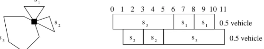
Quickly put, the reason for this latter property is as follows. Let us consider that the optimum solution of the linear relaxation contains the artificial variable with a certain valueσ that is not null. If there is an integer solution that does not contain the artificial trip, then the artificial variable can be set at 0 and the values of all other variables in the integer solution should be incremented byσ. This would improve the solution, which is absurd if it is optimal. An analytical proof of this statement can be found in Hernandez (2010).
0.5 vehicle 1 s2 s3 s3 3 s s2 2 s s1 1 s 11 10 9 8 7 6 5 4 3 2 1 0 0.5 vehicle s
Figure 2: Example of the non-existence of a feasible integer solution from a feasible fractional solution
3.3
Branch and Price scheme
The column generation scheme described above is embedded into a Branch and Price, i.e. a Branch and Bound algorithm is applied and, at each node of the search tree, column generation is carried out to compute a lower bound.
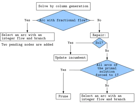
Two branching strategies are defined and used as follows. The first strategy is very common. An arc (i, j) with a fractional flow is selected (with the flow being the sum of the different flows generated by the path variables covering this arc). Two branches are created: one branch where the flow on arc (i, j)is forced to 1, one branch where it is forced to0. The selection rule for the arc is to select the arc whose fractional quantity of flow multiplied by its cost is maximized. Once finished, the two new nodes are added to the list of pending nodes, a new node is selected, column generation is applied and the branch-and-price scheme continues. New constraints (flows forced to 0 or 1) can be easily handled at the pricing and master problem levels by adequately removing arcs and variables.
Nevertheless, in our case, because of temporal constraints, having all arcs with an integer flow does not imply that the primal solution (set of θk variables) is an integer solution. It is indeed
possible that trips with identical structures but different timestamps are simultaneously selected in the solution (see Figure 2). When this situation occurs, the above branching strategy cannot be applied. We may thus adopt the second branching strategy, which is divided into two steps.
The first step is an attempt to obtain an integer solution that covers the set of arcs having a non-zero flow in the current primal solution. For this step, we introduce the so-called repair procedure detailed below. If an integer solution is found, it has the same cost as the current primal solution (the same arcs are covered with the same quantity of flow) and the search continues normally. Otherwise, that is when the repair procedure fails, no integer solution exists covering these arcs. We can thus deduce that at least one of these arcs is absent in the optimal solution. The second step then consists in successively searching for the best integer solution with one of the arcs forbidden. This step is carried out with the branching strategy detailed below.
Repair procedure (first step)
With a simple example, let us first show that constructing an integer solution from a fractional solution with integer flows on arcs is not always possible. Consider the fractional solution given in Figure 2, where:
• three structuress1, s2 and s3 are selected, with, for each structure, two trips of coefficient
0.5each,
• the durations of the structures (including loading) are2,2and 6respectively,
• the time windows of the three structures are[6,10],[1,5]and[0,11]respectively,
• a single vehicle is allowed.
This example clearly shows that no integer solution exists: none of the 6 possible sequences
{s1, s2, s3},{s1, s3, s2},{s2, s1, s3},{s2, s3, s1},{s3, s1, s2},{s3, s2, s1}admits a feasible schedule.
Actually, in this case (one vehicle), the problem of searching for a feasible solution is exactly
1|pi, ri,d˜i|−where tasks of durationpiwith release datesriand due datesd˜ihave to be scheduled
on a single machine. As this problem isN P−complete, see Lenstra et al. (1977), then the problem addressed with the repair procedure is alsoN P−complete.
Figure 3: Branching strategy
This problem can however be simply shaped as a VRPTW where the set of "customers" is the set of structures present in the current fractional solution (s1, s2, s3 on the above example).
Time windows associated with "customers"slare then set at[Al,Bl−dminl ]; service times, loading
times and demands are set at 0; and travel times on ongoing arcs from sl are set at dminl . The
repair procedure then consists in searching for a feasible solution for this VRPTW instance. If a solution is found, we update the incumbent solution and prune the node; otherwise, the second step is called for. We tackle the solution of this VRPTW with the branch-and-price algorithm described in Feillet et al. (2004). Note that repairing can be performed very quickly due to the size and characteristics of the VRPTW instance.
Branching strategy (second step)
When the repair procedure fails, it proves that finding an integer solution from the structures of the current primal solution is impossible. One can easily deduce that at least one of the arcs of these structures is not in the optimal solution. Indeed, otherwise, all arcs would be present in the optimal solution and, as these arcs are sufficient to cover the demand, the optimal solution would exactly match these arcs, which is impossible as shown by the repair procedure.
In order to forbid one of the arcs, we apply the standard branching rule for one of these arcs which has not been subject to any constraint yet: create two branches where the flow on the arc is forced to 0 and 1, respectively. Note that the effect of the branching will be nil on the branch where the flow is forced to 1. Hence, the branching will be repeated on this branch until pruning is activated or all arcs with flow 1are forced. In the latter case, the pending node can simply be removed as, from the repair procedure, we already know that no feasible solution can be obtained from this node.
Overall branching scheme
Figure 3 illustrates the overall branching scheme.
Remark about pruning:
The way we have defined the initial solution of the master problem, using an artificial variable defined above, allows us to prune some branches during the Branch and Price process thanks to
lemma 3.5. To make pruning even more efficient, the cost of this variable is set at the best known integer solution. This pruning condition proved effective during tests on Solomon’s instances, especially when there is no solution to cover the whole set of customers.
4
Results
4.1
Presentation
In this section, many results obtained with our exact algorithm are reported and compared to previous studies. First, the test instances of Solomon are presented. Then, we analyse the per-formance of our algorithm. The impact of the duration limit is also investigated. The computing platform is an Intel Core 2 duo 2.10 GHz with 2 GB of RAM using GLPK to solve the master problem. The computation time limit was set at2 hours.
4.2
Test instances
Our tests were performed using the well-known VRPTW benchmark instances created by Solomon (1987). These instances are divided into six classes that are a combination of two criteria. The first criterion concerns the spatial position of customers. There are three different spatial layouts: customers in clusters ("C" type), customers randomly located ("R" type), and an intermediate case with part of the customers clustered and the rest randomly located ("RC" type). The second criterion concerns the tightness of time constraints at customers. There are two types: tight time windows in a short planning time horizon (type "1") and large time windows in a long planning time horizon (type "2"). By combining these two criteria, there are six basic classes which are denoted: "C1", "C2", "R1", "R2", "RC1" and "RC2". Overall, there are 56 instances with 100 customers. Please note that for a given class, there are several instances with different customer time windows, but the spatial layout of customers is the same for the whole class. Instances are denoted as in the following example: C201-25 corresponds to the first instances of class "C2" where only the first 25 customers are considered. In this study, instances with a tight planning time horizon were discarded. In fact, the short horizon does not allow a significant number of routes to be assigned to the same vehicle.
The service time of the instances of class C2 (90) is much longer than the service time of instances of classes R2 and RC2(10). Therefore, tmax was set to 75for R2 and RC2 classes and
was set to 220 for the C2 class. These settings are consistent with the ones used in Azi et al. (2010). In order to check for the influence of a longer tmax than (75;220) on the comparison of
performances, algorithms are also tested for tmax set to (100;250).
Finally, for all instances, the customer loading time li was set at 20%of its service time sti,
and the fleet size was set to2 vehicles.
Note that, in the benchmark instances, only the customer and depot geolocalisations are given. Implicitly, the induced graph is considered complete and each edge receives a travel time that corresponds to the Euclidian distance between the corresponding nodes. In previous studies to which we compare our work, their respective authors used different numerical settings for the distances. In Azi et al. (2010) and Azi (2010), the authors truncated the distances at two decimal places. It appears that no truncation at all was applied to distances in Macedo et al. (2011). Yet, the authors rounded the distances of their solutions to two decimal places. The difference in truncating distances in the graph does not only change the results, it also affects the practical difficulty of each instance. Thus, in order to compare our algorithm with these two previous studies, we ran it with each of the two above-mentioned distance calculations. The results and comparison are given in two distinct sections and separate tables.
Note that our computing platform is an Intel Core 2 duo2.10GHz with2 GB of RAM using GLPK to solve the linear relaxation of the restricted master problem. The computing platform used in Azi (2010) is an AMD Opteron 3.1 GHz with 16GB of RAM using ILOG CPLEX 10.0 to solve the linear relaxation of the restricted master problem. The computing platform used in Macedo et al. (2011) 2.66 GHz Quad Core processor with 4 GB of RAM. Clearly, our machine is the least powerful of the three. For all instances, the computation time limit was set at 2 hours.
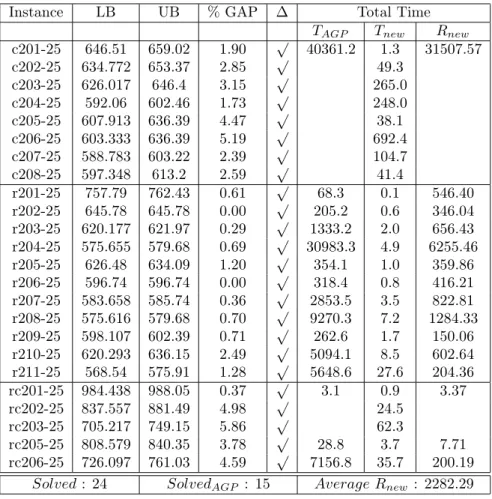
Instance LB UB % GAP ∆ Total Time
TAGP Tnew Rnew
c201-25 646.51 659.02 1.90 √ 40361.2 1.3 31507.57 c202-25 634.772 653.37 2.85 √ 49.3 c203-25 626.017 646.4 3.15 √ 265.0 c204-25 592.06 602.46 1.73 √ 248.0 c205-25 607.913 636.39 4.47 √ 38.1 c206-25 603.333 636.39 5.19 √ 692.4 c207-25 588.783 603.22 2.39 √ 104.7 c208-25 597.348 613.2 2.59 √ 41.4 r201-25 757.79 762.43 0.61 √ 68.3 0.1 546.40 r202-25 645.78 645.78 0.00 √ 205.2 0.6 346.04 r203-25 620.177 621.97 0.29 √ 1333.2 2.0 656.43 r204-25 575.655 579.68 0.69 √ 30983.3 4.9 6255.46 r205-25 626.48 634.09 1.20 √ 354.1 1.0 359.86 r206-25 596.74 596.74 0.00 √ 318.4 0.8 416.21 r207-25 583.658 585.74 0.36 √ 2853.5 3.5 822.81 r208-25 575.616 579.68 0.70 √ 9270.3 7.2 1284.33 r209-25 598.107 602.39 0.71 √ 262.6 1.7 150.06 r210-25 620.293 636.15 2.49 √ 5094.1 8.5 602.64 r211-25 568.54 575.91 1.28 √ 5648.6 27.6 204.36 rc201-25 984.438 988.05 0.37 √ 3.1 0.9 3.37 rc202-25 837.557 881.49 4.98 √ 24.5 rc203-25 705.217 749.15 5.86 √ 62.3 rc205-25 808.579 840.35 3.78 √ 28.8 3.7 7.71 rc206-25 726.097 761.03 4.59 √ 7156.8 35.7 200.19
Solved: 24 SolvedAGP : 15 Average Rnew: 2282.29
Table 1: Comparison of our results with Azi (2010) on Solomon’s benchmark (25 customers) with
tmax value set (75;220)
4.3
Results and comparison with Azi et al. (2010)
Tables 1, 2, 3 and 4 provide results with precision in distances in the graph set at two decimal places.
Tables 1 and 2 provide results fortmax set at (75; 220), for all instances with25 and 40
cus-tomers, respectively. Each table provides the lower bound (LB), the cost of the optimal solution (UB) that is found, the gap between these two values and the total solving time, in the subcolumn named Tnew. A "√ " in column ∆ indicates that the time instant relaxation provides a feasible
solution with the initial time granularity. A comparison of performances with (Azi (2010)) is pro-vided in the subcolumn named TAGP which is the processing time obtained in the study by Azi
(2010), and in the column named Rnew which is the ratio defined by the processing time in Azi
(2010) divided by the processing time of our method. Note that the results in Azi et al. (2010) were corrected in Azi (2010), which explains why we only compare with the latter. A "NoSol" in a table indicates that, with two vehicles, there is no solution covering all customers for the corresponding instance. A processing time in italics in the TAGP column indicates that the authors have found
a solution that does not cover all customers. WhenTAGP orTnewis left blank, the instance could
not be solved by the respective authors of the studies compared here. When none of the authors was able to find a solution, the instance is excluded from the table.
Our algorithm solves 47 of the 54 instances and the GAP between the lower and upper bounds ranges from0.00%to 5.86%. In all cases, the time instant relaxation was able to obtain feasible solutions with the initial time granularity. Only 22 were solved in Azi (2010). If we consider the instances for a which a coverage exists and which are solved by both methods, our algorithm gets significantly faster results, from3to 31000times faster, and2000times faster on average.
Tables 3 and 4 provide similar data as in the previous table, in the case of a longertmax, with
Instance LB UB % GAP ∆ Total Time
TAGP Tnew Rnew
c201-40 1124.31 1168.83 3.81 √ 19978.9 31.3 639.02 c202-40 1097.7 1111.15 1.21 √ 67.4 c203-40 1077.08 1088.55 1.05 √ 186.5 c204-40 1034.33 1039.16 0.46 √ 145.3 c205-40 1076.62 1083.81 0.66 √ 34.1 c206-40 1073.91 1081.37 0.69 √ 184.0 c207-40 1042.6 1055.04 1.18 √ 1491.5 c208-40 1063.72 1071.99 0.77 √ 3221.7 52.6 61.24 r201-40 NoSol NoSol √ 2979.5 0.5 r204-40 839.697 858.22 2.16 √ 4049.2 r205-40 991.896 1017.84 2.55 √ 244494.0 1193.4 204.87 r206-40 920.094 927.22 0.77 √ 171.5 r207-40 882.223 886.22 0.45 √ 68.9 r208-40 839.697 858.22 2.16 √ 4954.8 r209-40 926.303 935.81 1.02 √ 198.2 r210-40 937.597 952.92 1.61 √ 246.5 r211-40 849.855 869.75 2.29 √ 5093.9 rc201-40 NoSol NoSol √ 14.6 0.328 rc202-40 NoSol NoSol √ 6823.2 2.421 rc203-40 NoSol NoSol √ 5.8 rc205-40 NoSol NoSol √ 1904.2 0.859 rc206-40 NoSol NoSol √ 1.7 rc207-40 NoSol NoSol √ 4.1
Solved: 23 SolvedAGP : 7 Average Rnew : 301.71
Table 2: Comparison of our results with Azi (2010) on Solomon’s benchmark (40 customers) with
Instance LB UB % GAP ∆ Total Time
TAGP Tnew Rnew
c201-25 540.9 540.9 0.00 √ 1.3 0.1 10.40 c202-25 525.19 533.43 1.54 √ 51.4 c203-25 523.735 532.77 1.70 √ 335.7 c204-25 513.45 525.46 2.29 √ 4734.4 c205-25 522.05 529.94 1.49 √ 116.6 0.9 131.01 c206-25 516.162 527.84 2.21 √ 1987.2 123.9 16.04 c207-25 515.673 525.46 1.86 √ 31.1 c208-25 515.673 525.46 1.86 √ 4.7 r201-25 691.291 698.18 0.99 √ 43.6 0.8 55.83 r202-25 616.68 617.53 0.14 √ 25249.9 4.1 6216.13 r203-25 577.097 577.74 0.11 √ 75729.3 11.6 6523.33 r204-25 480.714 483.3 0.54 √ 33.6 r205-25 555.563 559.14 0.64 √ 1202.3 3.7 327.51 r206-25 523.64 523.64 0.00 √ 28498.1 5.7 4983.93 r207-25 497.421 512 2.85 √ 418.9 r208-25 477.029 483.3 1.30 √ 97.8 r209-25 511.943 517.69 1.11 √ 11173.9 14.1 791.97 r210-25 547.23 547.23 0.00 √ 26690.0 2.6 10167.62 r211-25 470.088 474.49 0.93 √ 80.4 rc201-25 814.062 849.33 4.15 √ 16.06 3.6 4.51 rc202-25 679.86 679.86 0.00 √ 1096.3 3.5 314.67 rc203-25 592.978 593.56 0.10 √ 13.1 rc205-25 698.723 702.49 0.54 √ 262.8 2.6 100.73 rc206-25 600.168 604.12 0.65 √ 222.7 2.9 77.46 rc207-25 510.509 514.81 0.84 √ 45.5
Solved: 25 SolvedAGP : 14 Average Rnew: 2122.94
Table 3: Comparison of our results with Azi (2010) on Solomon’s benchmark (25 customers) with
tmax value set (100;250)
Instance LB UB % GAP ∆ Total Time
TAGP Tnew Rnew
c201-40 934.564 966.7 3.32 √ 659.2 90.4 7.29 c202-40 914.099 919.85 0.63 √ 84.2 c205-40 911.751 921.19 1.02 √ 66.3 c206-40 911.027 919.05 0.87 √ 1539.1 c208-40 908.713 915.41 0.73 √ 2673.7 r201-40 NoSol NoSol √ 127424.0 15.5 r203-40 807.77 816.51 1.07 √ 2429.0 r205-40 852.379 872 2.25 √ 926.4 r206-40 803.272 812.31 1.11 √ 1511.4 r209-40 760.234 768.84 1.12 √ 479.8 rc201-40 NoSol NoSol √ 77.8 0.6 rc202-40 NoSol NoSol √ 10.3 rc205-40 NoSol NoSol √ 4733.3 4.2
Solved: 13 SolvedAGP : 4 Average Rnew : 7.29
Table 4: Comparison results with Azi (2010) on the Solomon’s benchmark (40 customers) with
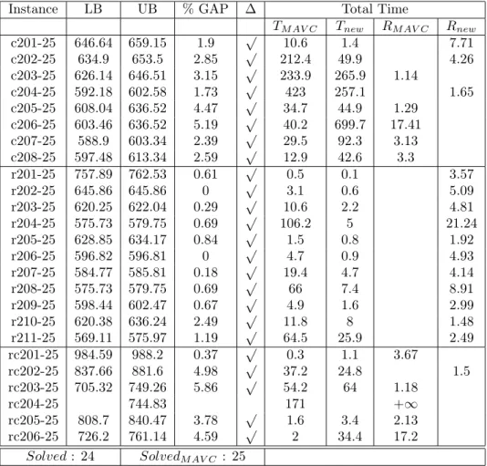
Instance LB UB % GAP ∆ Total Time TM AV C Tnew RM AV C Rnew c201-25 646.64 659.15 1.9 √ 10.6 1.4 7.71 c202-25 634.9 653.5 2.85 √ 212.4 49.9 4.26 c203-25 626.14 646.51 3.15 √ 233.9 265.9 1.14 c204-25 592.18 602.58 1.73 √ 423 257.1 1.65 c205-25 608.04 636.52 4.47 √ 34.7 44.9 1.29 c206-25 603.46 636.52 5.19 √ 40.2 699.7 17.41 c207-25 588.9 603.34 2.39 √ 29.5 92.3 3.13 c208-25 597.48 613.34 2.59 √ 12.9 42.6 3.3 r201-25 757.89 762.53 0.61 √ 0.5 0.1 3.57 r202-25 645.86 645.86 0 √ 3.1 0.6 5.09 r203-25 620.25 622.04 0.29 √ 10.6 2.2 4.81 r204-25 575.73 579.75 0.69 √ 106.2 5 21.24 r205-25 628.85 634.17 0.84 √ 1.5 0.8 1.92 r206-25 596.82 596.81 0 √ 4.7 0.9 4.93 r207-25 584.77 585.81 0.18 √ 19.4 4.7 4.14 r208-25 575.73 579.75 0.69 √ 66 7.4 8.91 r209-25 598.44 602.47 0.67 √ 4.9 1.6 2.99 r210-25 620.38 636.24 2.49 √ 11.8 8 1.48 r211-25 569.11 575.97 1.19 √ 64.5 25.9 2.49 rc201-25 984.59 988.2 0.37 √ 0.3 1.1 3.67 rc202-25 837.66 881.6 4.98 √ 37.2 24.8 1.5 rc203-25 705.32 749.26 5.86 √ 54.2 64 1.18 rc204-25 744.83 171 +∞ rc205-25 808.7 840.47 3.78 √ 1.6 3.4 2.13 rc206-25 726.2 761.14 4.59 √ 2 34.4 17.2 Solved: 24 SolvedM AV C : 25
Table 5: Comparison of our results with Macedo et al. (2011) on Solomon’s benchmark (25 cus-tomers) withtmaxvalue set (75;220)
Our algorithm solves38of54instances with a GAP that ranges from0.00%to4.15%and all solutions are found during the first resolution, whereas in Azi (2010) only 18 are solved. As for the smaller tmax case, if we consider instances where there is complete coverage for instances solved
by both methods, our algorithm is 2000 times faster on average for these instances than the one given in Azi (2010), and the ratio ranges from5times faster to 10000times faster.
4.4
Results and comparison with Macedo et al. (2011)
Following the results and comparison with the first published algorithm on MTVRPTW-LD, we provide here a comparison with the results given in the second and very recent work of Macedo et al. (2011). As already explained, separate comparison could not be avoided due to the different numerical settings for distance calculations.
Tables 5, 6, 7 and 8 provide results based on distance calculations that do not include any rounding.
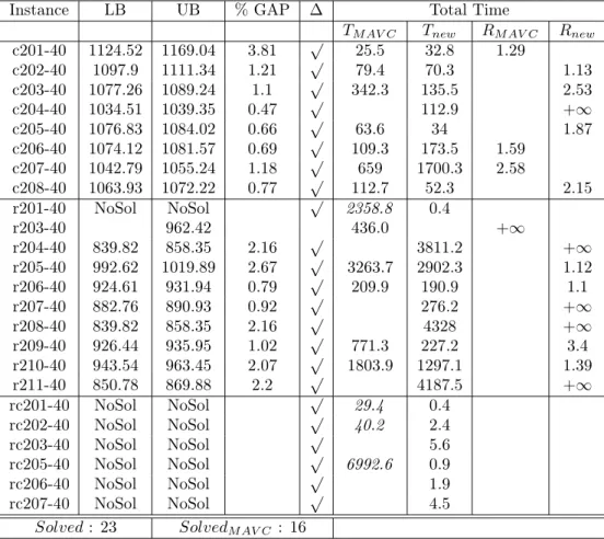
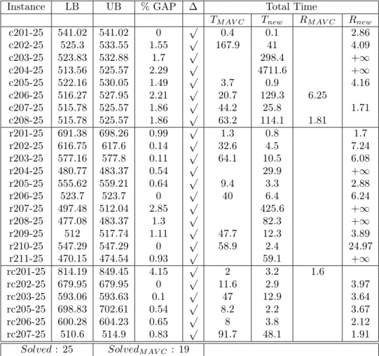
Tables 5, 6, 7 and 8 provide results for tmax set at(75; 220)and(100; 250), for every instance
with 25 and 40 customers. The columns are defined as in the previous section, except for the "Total Time" column that is decomposed into four subcolumns: TM AV C, Tnew, RM AV C and
Rnew. TM AV C andTnew indicate the processing time of the algorithm published in Macedo et al.
(2011) and the processing time of our algorithm, respectively. RM AV C and Rnew give ratios of
the computing times of the slowest method divided by the fastest; depending on which method is the fastest, the ratio is reported in one column or in the other. A value +∞ is reported when a single method solves the instance. A "NoSol" in a table indicates that, with two vehicles, there is no solution covering all customers for the corresponding instance. A "√" in column∆ indicates that the time instant relaxation provides a feasible solution with the initial time granularity. A
Instance LB UB % GAP ∆ Total Time TM AV C Tnew RM AV C Rnew c201-40 1124.52 1169.04 3.81 √ 25.5 32.8 1.29 c202-40 1097.9 1111.34 1.21 √ 79.4 70.3 1.13 c203-40 1077.26 1089.24 1.1 √ 342.3 135.5 2.53 c204-40 1034.51 1039.35 0.47 √ 112.9 +∞ c205-40 1076.83 1084.02 0.66 √ 63.6 34 1.87 c206-40 1074.12 1081.57 0.69 √ 109.3 173.5 1.59 c207-40 1042.79 1055.24 1.18 √ 659 1700.3 2.58 c208-40 1063.93 1072.22 0.77 √ 112.7 52.3 2.15 r201-40 NoSol NoSol √ 2358.8 0.4 r203-40 962.42 436.0 +∞ r204-40 839.82 858.35 2.16 √ 3811.2 +∞ r205-40 992.62 1019.89 2.67 √ 3263.7 2902.3 1.12 r206-40 924.61 931.94 0.79 √ 209.9 190.9 1.1 r207-40 882.76 890.93 0.92 √ 276.2 +∞ r208-40 839.82 858.35 2.16 √ 4328 +∞ r209-40 926.44 935.95 1.02 √ 771.3 227.2 3.4 r210-40 943.54 963.45 2.07 √ 1803.9 1297.1 1.39 r211-40 850.78 869.88 2.2 √ 4187.5 +∞ rc201-40 NoSol NoSol √ 29.4 0.4 rc202-40 NoSol NoSol √ 40.2 2.4 rc203-40 NoSol NoSol √ 5.6 rc205-40 NoSol NoSol √ 6992.6 0.9 rc206-40 NoSol NoSol √ 1.9 rc207-40 NoSol NoSol √ 4.5 Solved: 23 SolvedM AV C : 16
Table 6: Comparison of our results with Macedo et al. (2011) on Solomon’s benchmark (40 cus-tomers) withtmaxvalue set (75;220)
processing time in italics in column TM AV C (tables 6 and 8) indicates that the authors found a
solution that does not cover all customers. WhenTM AV C orTnew is left blank, the instance could
not be solved by the respective authors of the studies compared here. When none of the authors was able to find a solution, the instance is excluded from the table.
Our algorithm closes 86 of the 108 instances and the GAP between the lower and upper bounds ranges from0.00%to5.86%. As for the comparaison with Azi (2010), all solutions found during the resolution of the relaxed time instant case are optimal. In Macedo et al. (2011), only 67 instances of this set were solved.
Our algorithm clearly performed better than that of Macedo et al. (2011), particulary for instances of the Rclass. The new algorithm solves all R instances for25customers for short and longertmax. The algorithm in Macedo et al. (2011) does not solve4of these, which have a longer
tmax. ForR instances commonly solved and for which there is complete client coverage, the total
solving time of our algorithm is approximately 97 seconds whereas the total for that in Macedo et al. (2011) is approximately 547seconds. Solving is faster by an average factor of5. When it comes to instances of theRclass and40customers, our algorithm closes15instances whereas that of Macedo et al. (2011) only closes6. The difference is highest for the longesttmax.
A comparison of the two algorithms for theC class does not exhibit significant advantages of one algorithm. Our algorithm closes more instances (29compared to25), but the fastest algorithm depends much on a particular instance.
The situation for theRCclass is also closely dependent on a given instance for the comparison of solving times. For the 11 commonly solved instances with complete coverage our algorithm performs better in 6 cases. Among the three algorithms compared in this paper, the algorithm published in Macedo et al. (2011) is the only one that closes the instance RC204−25 for the shortertmax.
Finally, our algorithm clearly performs better than that of Macedo et al. (2011) when the number of customers or the limit durationtmaxare increased.
5
Conclusions
Our algorithm compares very favorably with the first algorithm published on the MTVRPTW-LD, Azi et al. (2010). It also outperforms the more recent one, Macedo et al. (2011), on instances of theRclass. There are instances in theRandRC classes in which the algorithm given in Macedo et al. (2011) has the best performance to date. Compared to Azi et al. (2010), a main advantage of our approach lies in the efficiency of the Column Generation subproblem, which is solved with a fast pseudo-polynomial algorithm. The time-indexed graph introduced in Macedo et al. (2011) seems to have some advantages for some clustered clients layouts. It follows that this feature might be combined with our own approach to further improve exact solution of MTVRPTW-LD. Our approach is more robust with respect to longertmax and the number of customers than previous
works.
With the instances considered, all solutions found when solving the time instant relaxation of the problem happen to be feasible in the unrelaxed problem. This indicates that this relaxation is very efficient.
The solving time is extremely variable between instances of the same class. In order to allow precise comparisons and design faster techniques, a successor to the classic Solomon (1987) bench-mark would benefit the community. Future research should address exact solution of MTVRPTW for cases without limited trip duration.
Acknowledgment
We thank referees for several insightful comments that helped improving the readability of this paper. We thank IRSTEA and Région Languedoc-Roussillon in France for providing the basic funding of this research, as well as contributions from the LIRMM, PNRB MOBIPE project sup-ported by the french ANR, and A2PV SyDeReT project. Finally, we are grateful to Pr J.C. König for his support during this work.
Instance LB UB % GAP ∆ Total Time TM AV C Tnew RM AV C Rnew c201-25 541.02 541.02 0 √ 0.4 0.1 2.86 c202-25 525.3 533.55 1.55 √ 167.9 41 4.09 c203-25 523.83 532.88 1.7 √ 298.4 +∞ c204-25 513.56 525.57 2.29 √ 4711.6 +∞ c205-25 522.16 530.05 1.49 √ 3.7 0.9 4.16 c206-25 516.27 527.95 2.21 √ 20.7 129.3 6.25 c207-25 515.78 525.57 1.86 √ 44.2 25.8 1.71 c208-25 515.78 525.57 1.86 √ 63.2 114.1 1.81 r201-25 691.38 698.26 0.99 √ 1.3 0.8 1.7 r202-25 616.75 617.6 0.14 √ 32.6 4.5 7.24 r203-25 577.16 577.8 0.11 √ 64.1 10.5 6.08 r204-25 480.77 483.37 0.54 √ 29.9 +∞ r205-25 555.62 559.21 0.64 √ 9.4 3.3 2.88 r206-25 523.7 523.7 0 √ 40 6.4 6.24 r207-25 497.48 512.04 2.85 √ 425.6 +∞ r208-25 477.08 483.37 1.3 √ 82.3 +∞ r209-25 512 517.74 1.11 √ 47.7 12.3 3.89 r210-25 547.29 547.29 0 √ 58.9 2.4 24.97 r211-25 470.15 474.54 0.93 √ 59.1 +∞ rc201-25 814.19 849.45 4.15 √ 2 3.2 1.6 rc202-25 679.95 679.95 0 √ 11.6 2.9 3.97 rc203-25 593.06 593.63 0.1 √ 47 12.9 3.64 rc205-25 698.83 702.61 0.54 √ 8.2 2.2 3.67 rc206-25 600.28 604.23 0.65 √ 8 3.8 2.12 rc207-25 510.6 514.9 0.83 √ 91.7 48.1 1.91 Solved: 25 SolvedM AV C : 19
Table 7: Comparison of our results with Macedo et al. (2011) on Solomon’s benchmark (25 cus-tomers) withtmaxvalue set (100;250)
Instance LB UB % GAP ∆ Total Time
TM AV C Tnew RM AV C Rnew c201-40 934.76 966.89 3.32 √ 6.4 85.4 13.34 c202-40 914.28 920.05 0.63 √ 81.1 +∞ c205-40 911.93 921.37 1.02 √ 88.5 54.8 1.62 c206-40 911.21 919.24 0.87 √ 290.5 1522.2 5.24 c208-40 908.89 915.61 0.73 √ 491.5 2582.7 5.25 r201-40 NoSol NoSol √ 13.2 r203-40 807.91 816.65 1.07 √ 2469.1 +∞ r205-40 852.51 873.36 2.39 √ 1200.4 +∞ r206-40 803.4 812.42 1.11 √ 1514.2 +∞ r207-40 752.33 764.52 1.59 √ 7029.8 +∞ r209-40 760.38 768.99 1.12 √ 454 +∞ rc201-40 NoSol NoSol √ 3.6 0.8 rc202-40 NoSol NoSol √ 1013.8 10.4 rc205-40 NoSol NoSol √ 35.7 3.9 Solved: 14 SolvedM AV C : 7
Table 8: Comparison of our results with Macedo et al. (2011) on Solomon’s benchmark (40 cus-tomers) withtmaxvalue set (100;250)
References
Azi, N. 2010. Méthodes exactes et heuristiques pour le problème de tournées avec fenêtres de temps et réutilisation de véhicules. Ph.D. thesis, Université de Montréal.
Azi, N., M. Gendreau, J.-Y. Potvin. 2007. An exact algorithm for a single-vehicle routing problem with time windows and multiple routes. European Journal of Operational Research178(3) 755–766. Azi, N., M. Gendreau, J.-Y. Potvin. 2010. An exact algorithm for a vehicle routing problem with time
windows and multiple use of vehicles. European Journal of Operational Research202(3) 756–763.
Barnhart, C., E.L. Johnson, G.L. Nemhauser, M.W.P. Savelsbergh, P.H. Vance. 1996. Branch-and-price: Column generation for solving huge integer programs. Operations Research 46316–329.
Battarra, M., M. Monaci, D. Vigo. 2009. An adaptive guidance approach for the heuristic solution of a minimum multiple trip vehicle routing problem. Computers & Operations Research 36(11) 3041– 3050.
Desrochers, M., J. Desrosiers, M. Solomon. 1992. A new optimization algorithm for the vehicle-routing problem with time windows. Operations Research 40(2) 342–354.
Feillet, D. 2010. A tutorial on column generation and branch-and-price for vehicle routing problems. 4OR - A Quarterly Journal of Operations Research 8(2) 407–424.
Feillet, D., P. Dejax, M. Gendreau, C. Gueguen. 2004. An exact algorithm for the elementary shortest path problem with resource constraints: Application to some vehicle routing problems. Networks
44(3) 216–229.
Fleischmann, B. 1990. The vehicle routing problem with multiple use of vehicles. Working paper, Fach-bereich Wirtshaftswissenschaften, Universität Hamburg.
Hernandez, F. 2010. Méthodes de résolution exactes pour le problème de routage de véhicules avec fenêtres de temps et routes multiples. Phd thesis in french, Montpellier II University.
Lenstra, J.K., A.H.G. Rinnooy Kan, P. Brucker. 1977. Complexity of scheduling machine problems.Annales of Discrete Mathematics 1343–362.
Macedo, R., C. Alves, J. M. Valério de Carvalho, F. Clautiaux, S. Hanafi. 2011. Solving the vehicle routing problem with time windows and multiple routes exactly using a pseudo-polynomial model. European Journal of Operational Research 214(3) 536–545.
Mingozzi, A., R. Roberti, P. Toth. 2012. An exact algorithm for the multi-trip vehicle routing problem.
INFORMS Journal on Computing 757–759.
Sen, A., K. Bülbül. 2008. A survey on multiple vehicle routing problem.International Logistics and Supply Chain Congress’ 2008. Istanbul, TURKEY.
Solomon, M.M. 1987. Algorithms for the vehicle routing and scheduling problem with time window con-straints. Operations Research 35254–265.